Japan Advanced Institute of Science and Technology
JAIST Repository
https://dspace.jaist.ac.jp/
Title
Polynomial Interpretations with Negative
Coefficients
Author(s)
Hirokawa, Nao; Middeldorp, Aart
Citation
Lecture Notes in Computer Science, 3249/2004:
185-198
Issue Date
2004
Type
Journal Article
Text version
author
URL
http://hdl.handle.net/10119/9059
Rights
This is the author-created version of Springer,
Nao Hirokawa and Aart Middeldorp, Lecture Notes
in Computer Science, 3249/2004, 2004, 185-198.
The original publication is available at
www.springerlink.com,
http://dx.doi.org/10.1007/b100361
Description
Proceedings of the 7th International Conference,
AISC 2004, Linz, Austria, September 22-24, 2004.
Polynomial Interpretations with Negative Coefficients
Nao Hirokawa and Aart Middeldorp
Institute of Computer Science University of Innsbruck 6020 Innsbruck, Austria
{nao.hirokawa,aart.middeldorp}@uibk.ac.at
Abstract. Polynomial interpretations are a useful technique for proving termination of term rewrite systems. We show how polynomial interpre-tations with negative coefficients, like x − 1 for a unary function symbol or x − y for a binary function symbol, can be used to extend the class of rewrite systems that can be automatically proved terminating.
1
Introduction
This paper is concerned with automatically proving termination of first-order rewrite systems by means of polynomial interpretations. In the classical ap-proach, which goes back to Lankford [16], one associates with every n-ary func-tion symbol f a polynomial Pf over the natural numbers in n indeterminates,
which induces a mapping from terms to polynomials in the obvious way. Then one shows that for every rewrite rule l → r the polynomial Pl associated with
the left-hand side l is strictly greater than the polynomial Prassociated with the
right-hand side r, i.e., Pl−Pr>0 for all values of the indeterminates. In order to
conclude termination, the polynomial Pf associated with an n-ary function
sym-bol f must be strictly monotone in all n indeterminates. Techniques for finding appropriate polynomials as well as approximating (in general undecidable) poly-nomial inequalities P > 0 are described in several papers (e.g. [4, 6, 9, 15, 19]). As a simple example, consider the rewrite rules
x+ 0 → x x× 0 → 0
x+ s(y) → s(x + y) x× s(y) → (x × y) + x
Termination can be shown by the strictly monotone polynomial interpretations ×N(x, y) = 2xy + y + 1 +N(x, y) = x + 2y sN(x) = x + 1 0N= 1
over the natural numbers:
x+ 2 > x 2x + 2 > 1
x+ 2y + 2 > x + 2y + 1 2xy + 2x + y + 2 > 2xy + 2x + y + 1 Compared to other classical methods for proving termination of rewrite sys-tems (like recursive path orders and Knuth-Bendix orders), polynomial interpre-tations are rather weak. Numerous natural examples cannot be handled because
of the strict monotonicity requirement which precludes interpretations like x + 1 for binary function symbols. In connection with the dependency pair method of Arts and Giesl [1], polynomial interpretations become much more useful be-cause strict monotonicity is no longer required; weak monotonicity is sufficient and hence x + 1 or even 0 as interpretation of a binary function symbol causes no problems. Monotonicity is typically guaranteed by demanding that all coef-ficients are positive.
In this paper we go a step further. We show that polynomial interpretations over the integers with negative coefficients like x − 1 and x − y + 1 can also be used for termination proofs. To make the discussion more concrete, let us consider a somewhat artificial example: the recursive definition
f(x) = if x > 0 then f (f (x − 1)) + 1 else 0
from [8]. It computes the identity function over the natural numbers. Termina-tion of the rewrite system
1 : f(s(x)) → s(f(f(p(s(x))))) 2 : f(0) → 0 3 : p(s(x)) → x obtained after the obvious translation is not easily proved. The (manual) proof in [8] relies on forward closures whereas powerful automatic tools like AProVE [11] and CiME [5] that incorporate both polynomial interpretations and the depen-dency pair method fail to prove termination. There are three dependepen-dency pairs (here f]and p] are new function symbols):
4 : f](s(x)) → f](f(p(s(x)))) 5 : f](s(x)) → f](p(s(x))) 6 : f](s(x)) → p](s(x))
By taking the natural polynomial interpretation
fZ(x) = fZ](x) = x sZ(x) = x + 1 0Z= 0 pZ(x) = p]Z(x) = x − 1
over the integers, the rule and dependency pair constraints reduce to the follow-ing inequalities:
1 : x + 1 > x + 1 3 : x> x 5 : x + 1 > x 2 : 0 > 0 4 : x + 1 > x 6 : x + 1 > x
These constraints are obviously satisfied. The question is whether we are al-lowed to conclude termination at this point. We will argue that the answer is affirmative and, moreover, that the search for appropriate natural polynomial interpretations can be efficiently implemented.
The approach described in this paper is inspired by the combination of the general path order and forward closures [8] as well as semantic labelling [24]. Concerning related work, Lucas [17, 18] considers polynomials with real coef-ficients for automatically proving termination of (context-sensitive) rewriting systems. He solves the problem of well-foundedness by replacing the standard order on R with >δfor some fixed positive δ ∈ R: x >δ yif and only if x − y > δ.
(i.e., there exists an m ∈ R such that fR(x1, . . . , xn) > m for all function symbols
f and x1, . . . , xn > m). The latter requirement entails that interpretations like
x− 1 or x − y + 1 cannot be handled.
The remainder of the paper is organized as follows. In Section 3 we discuss polynomial interpretations with negative constants. Polynomial interpretations with negative coefficients require a different approach, which is detailed in Sec-tion 4. In SecSec-tion 5 we discuss briefly how to find suitable polynomial interpreta-tions automatically and we report on the many experiments that we performed.
2
Preliminaries
We assume familiarity with the basics of term rewriting [3, 21] and with the dependency pair method [1] for proving (innermost) termination. In the latter method a term rewrite system (TRS for short) is transformed into a collection of ordering constraints of the form l & r and l > r that need to be solved in order to conclude termination. Solutions (&, >) must be reduction pairs which consist of a rewrite preorder & (i.e., a transitive and reflexive relation which is closed under contexts and substitutions) on terms and a compatible well-founded order > which is closed under substitutions. Compatibility means that the inclusion & · > ⊆ > or the inclusion > · & ⊆ > holds. (Here · denotes relational composition.)
A general semantic construction of reduction pairs, which covers traditional polynomial interpretations, is based on the concept of algebra. If we equip the carrier A of an F-algebra A = (A, {fA}f ∈F) with a well-founded order > such
that every interpretation function is weakly monotone in all arguments (i.e., fA(x1, . . . , xn) > fA(y1, . . . , yn) whenever xi> yi for all 1 6 i 6 n, for every
n-ary function symbol f ∈ F) then (>A, >A) is a reduction pair. Here the relations
>A and >A are defined as follows: s >A t if [α]A(s) > [α]A(t) and s >A t if
[α]A(s) > [α]A(t), for all assignments α of elements of A to the variables in s
and t ([α]A(·) denotes the usual evaluation function associated with the algebra
A). In general, the relation >A is not closed under contexts, >A is a preorder
but not a partial order, and >Ais not the strict part of >A. Compatibility holds
because of the identity >A· >A = >A. We write s =A t if [α]A(s) = [α]A(t)
for all assignments α. We say that A is a model for a TRS R if l =A r for all
rewrite rules in R.
In this paper we use the following results from [10] concerning dependency pairs.
Theorem 1. A TRS R is terminating if for every cycle C in its dependency graph there exists a reduction pair (&, >) such that R ⊆ &, C ⊆ & ∪ >, and
C ∩ > 6= ∅. ut
Theorem 2. A TRSR is innermost terminating if for every cycle C in its in-nermost dependency graph there exists a reduction pair(&, >) such that U(C) ⊆
3
Negative Constants
3.1 Theoretical Framework
When using polynomial interpretations with negative constants like in the ex-ample of the introduction, the first challenge we face is that the standard order > on Z is not well-founded. Restricting the domain to the set N of natural numbers makes an interpretation like pZ(x) = x − 1 ill-defined. Dershowitz and
Hoot observe in [8] that if all (instantiated) subterms in the rules of the TRS are interpreted as non-negative integers, such interpretations can work correctly. Following their observation, we propose to modify the interpretation of p to pN(x) = max{0, x − 1}.
Definition 3. LetF be a signature and let (Z, {fZ}f ∈F) be an F-algebra such
that every interpretation function fZ is weakly monotone in all its arguments.
The interpretation functions of the induced algebra (N, {fN}f ∈F) are defined as
follows: fN(x1, . . . , xn) = max{0, fZ(x1, . . . , xn)} for all x1, . . . , xn∈ N.
With respect to the interpretations in the introduction we obtain sN(pN(x)) =
max{0, max{0, x − 1} + 1} = max{0, x − 1} + 1, pN(0N) = max{0, 0} = 0, and
pN(sN(x)) = max{0, max{0, x + 1} − 1} = x.
Lemma 4. If (Z, {fZ}f ∈F) is an F-algebra with weakly monotone
interpreta-tions then(>N, >N) is a reduction pair.
Proof. It is easy to show that the interpretation functions of the induced alge-bra are weakly monotone in all arguments. Routine arguments reveal that the relation >Nis a well-founded order which is closed under substitutions and that
>Nis a preorder closed under contexts and substitutions. Moreover, the identity
>N· >N= >Nholds. Hence (>N, >N) is a reduction pair. ut
It is interesting to remark that unlike usual polynomial interpretations, the relation >N does not have the (weak) subterm property. For instance, with
re-spect to the interpretations in the example of the introduction, we have s(0) >N
p(s(0)) and not p(s(0)) >Np(0).
In recent modular refinements of the dependency pair method [23, 13, 22] suitable reduction pairs (&, >) have to satisfy the additional property of CE
-compatibility: & must orient the rules of the TRS CE consisting of the two
rewrite rules cons(x, y) → x and cons(x, y) → y, where cons is a fresh func-tion symbol, from left to right. This is not a problem because we can simply define consN(x, y) = max{x, y}. In this way we obtain a reduction pair (%, )
on terms over the original signature extended with cons such that & ∪ CE ⊆ %
and > ⊆ .
Example 5. Consider the TRS consisting of the following rewrite rules:
1 : half(0) → 0 4 : bits(0) → 0
2 : half(s(0)) → 0 5 : bits(s(x)) → s(bits(half(s(x)))) 3 : half(s(s(x))) → s(half(x))
The function half(x) computes dx
2e and bits(x) computes the number of bits that
are needed to represent all numbers less than or equal to x. Termination of this TRS is proved in [2] by using the dependency pair method together with the narrowing refinement. There are three dependency pairs:
6 : half](s(s(x))) → half](x)
7 : bits](s(x)) → bits](half(s(x))) 8 : bits](s(x)) → half](s(x))
By taking the interpretations 0Z= 0, halfZ(x) = x − 1, bitsZ(x) = half]Z(x) = x,
and sZ(x) = bits]Z(x) = x + 1, we obtain the following constraints over N:
1 : 0 > 0 5 : x+ 1 > x + 1
2 : 0 > 0 6 : x+ 2 > x
3 : x+ 1 > max{0, x − 1} + 1 7 : x+ 2 > x + 1
4 : 0 > 0 8 : x+ 2 > x + 1
These constraints are satisfied, so the TRS is terminating, but how can an in-equality like x + 1 > max{0, x − 1} + 1 be verified automatically?
3.2 Towards Automation
Because the inequalities resulting from interpretations with negative constants may contain the max operator, we cannot use standard techniques for comparing polynomial expressions. In order to avoid reasoning by case analysis (x − 1 > 0 or x − 1 6 0 for constraint 3 in Example 5), we approximate the evaluation function of the induced algebra.
Definition 6. Given a polynomial P with coefficients in Z, we denote the con-stant part by c(P ) and the non-concon-stant part P −c(P ) by n(P ). Let (Z, {fZ}f ∈F)
be anF-algebra such that every fZis a weakly monotone polynomial. With every
term t we associate polynomials Pleft(t) and Pright(t) with coefficients in Z and
variables in t as indeterminates: Pleft(t) = t if t is a variable 0 if t= f (t1, . . . , tn), n(P1) = 0, and c(P1) < 0 P1 otherwise
where P1= fZ(Pleft(t1), . . . , Pleft(tn)) and
Pright(t) = t if t is a variable n(P2) if t= f (t1, . . . , tn) and c(P2) < 0 P2 otherwise
where P2 = fZ(Pright(t1), . . . , Pright(tn)). Let α : V → N be an assignment. The
result of evaluating Pleft(t) and Pright(t) under α is denoted by [α]lZ(t) and
[α]r
According the following lemma, Pleft(t) is a lower bound and Pright(t) is an
upper bound of the interpretation of t in the induced algebra.
Lemma 7. Let (Z, {fZ}f ∈F) be an F-algebra such that every fZ is a weakly
monotone polynomial. Let t be a term. For every assignment α: V → N we have [α]r
Z(t) > [α]N(t) > [α]lZ(t).
Proof. By induction on the structure of t. If t ∈ V then [α]r
Z(t) = [α]lZ(t) =
α(t) = [α]N(t). Suppose t = f (t1, . . . , tn). According to the induction hypothesis,
[α]r
Z(ti) > [α]N(ti) > [α]lZ(ti) for all i. Since fZis weakly monotone,
fZ([α]rZ(t1), . . . , [α]rZ(tn)) > fZ([α]N(t1), . . . , [α]N(tn)) > fZ([α]Zl(t1), . . . , [α]lZ(tn))
By applying the weakly monotone function max{0, ·} we obtain max{0, α(P2)} >
[α]N(t) > max{0, α(P1)} where P1 = fZ(Pleft(t1), . . . , Pleft(tn)) and P2 =
fZ(Pright(t1), . . . , Pright(tn)). We have
[α]lZ(t) = ( 0 if n(P1) = 0 and c(P1) < 0 α(P1) otherwise and thus [α]l Z(t) 6 max{0, α(P1)}. Likewise, [α]rZ(t) = ( α(n(P2)) if c(P2) < 0 α(P2) otherwise
In the former case, α(n(P2)) = α(P2) − c(P2) > α(P2) and α(n(P2)) > 0. In the
latter case α(P2) > 0. So in both cases we have [α]rZ(t) > max{0, α(P2)}. Hence
we obtain the desired inequalities. ut
Corollary 8. Let (Z, {fZ}f ∈F) be an F-algebra such that every fZ is a weakly
monotone polynomial. Let s and t be terms. If Pleft(s)−Pright(t) > 0 then s >Nt.
If Pleft(s) − Pright(t) > 0 then s >Nt. ut
Example 9. Consider again the TRS of Example 5. By applying Pleft to the
left-hand sides and Pright to the right-hand sides of the rewrite rules and the
dependency pairs, the following ordering constraints are obtained:
1 : 0 > 0 3 : x + 1 > x + 1 5 : x + 1 > x + 1 7 : x + 2 > x + 1 2 : 0 > 0 4 : 0 > 0 6 : x + 2 > x 8 : x + 2 > x + 1 The only difference with the constraints in Example 5 is the interpretation of the term s(half(x)) on the right-hand side of rule 3. We have Pright(half(x)) =
n(x − 1) = x and thus Pright(s(half(x))) = x + 1. Although x + 1 is less precise
than max{0, x − 1} + 1, it is accurate enough to solve the ordering constraint resulting from rule 3.
So once the interpretations fZ are determined, we transform a rule l → r
into the polynomial Pleft(l) − Pright(r). Standard techniques can then be used
to test whether this polynomial is positive (or non-negative) for all values in N for the variables. The remaining question is how to find suitable interpretations for the function symbols. This problem will be discussed in Section 5.
4
Negative Coefficients
Let us start with an example which shows that negative coefficients in polynomial interpretations can be useful.
Example 10. Consider the following variation of a TRS in [2]:
1 : 06 x→ true 7 : x− 0 → x
2 : s(x) 6 0 → false 8 : s(x) − s(y) → x − y 3 : s(x) 6 s(y) → x 6 y 9 : if(true, x, y) → x 4 : mod(0, s(y)) → 0 10 : if(false, x, y) → y 5 : mod(s(x), 0) → 0
6 : mod(s(x), s(y)) → if(y 6 x, mod(s(x) − s(y), s(y)), s(x)) There are 6 dependency pairs:
11 : s(x) 6]s(y) → x 6]y
12 : s(x) −]s(y) → x −]y
13 : mod](s(x), s(y)) → if](y 6 x, mod(s(x) − s(y), s(y)), s(x)) 14 : mod](s(x), s(y)) → y 6]x
15 : mod](s(x), s(y)) → mod](s(x) − s(y), s(y)) 16 : mod](s(x), s(y)) → s(x) −]s(y)
Since the TRS is non-overlapping, it is sufficient to prove innermost termination. The problematic cycle in the (innermost) dependency graph is C = {15}. The usable rewrite rules for this cycle are U(C) = {7, 8}. We need to find a reduction pair (&, >) such that rules 4 and 5 are weakly decreasing (i.e., compatible with &) and dependency pair 15 is strictly decreasing (with respect to >). The only way to achieve the latter is by using the observation that s(x) is semantically greater than the syntactically larger term s(x)−s(y). If we take the natural interpretation −Z(x, y) = x − y, sZ(x) = x − 1, and 0Z= 0, together with mod]Z(x, y) = x then
we obtain the following ordering constraints over the natural numbers: 7 : x > x 8 : max{0, x − y} > max{0, x − y} 15 : x + 1 > max{0, x − y} 4.1 Theoretical Framework
The constraints in the above example are obviously satisfied, but are we allowed to use an interpretation like −Z(x, y) = x − y in (innermost) termination proofs?
The answer appears to be negative because Lemma 4 no longer holds. Because the induced interpretation −N(x, y) = max{0, x − y} is not weakly monotone in
its second argument, the order >N of the induced algebra is not closed under
contexts, so if s >N t then it may happen that C[s] 6N C[t]. Consequently,
s >N t, closure under contexts is obtained for free. So we could take (=N, >N)
as reduction pair. This works fine in the above example because the induced algebra is a model of the set of usable rules {7, 8} and >N orients dependency
pair 15. However, requiring that all dependency pairs in a cycle are compatible with =N∪>Nis rather restrictive because dependency pairs that are transformed
into a polynomial constraint of the form x2
> x or x + 2y > x + y cannot be handled. So we will allow >Nfor the orientation of dependency pairs in a cycle
C but insist that at least one dependency pair in C is compatible with >N. (Note
that the relation =N∪ >N is properly contained in >N.) The theorems below
state the soundness of this approach in a more abstract setting. The proofs are straightforward modifications from the ones in [13]. The phrase “there are no minimal C-rewrite sequences” intuitively means that if a TRS R is non-terminating then this is due to a different cycle of the dependency graph. Theorem 11. LetR be a TRS and let C be a cycle in its dependency graph. If there exists an algebraA equipped with a well-founded order > such that R ⊆ =A,
C ⊆ >A, andC ∩ >A6= ∅ then there are no minimal C-rewrite sequences. ut
In other words, when proving termination, a cycle C of the dependency graph can be ignored if the conditions of Theorem 11 are satisfied. A similar statement holds for innermost termination.
Theorem 12. LetR be a TRS and let C be a cycle in its innermost dependency graph. If there exists an algebra A equipped with a well-founded order > such thatU(C) ⊆ =A,C ⊆ >A, andC ∩ >A6= ∅ then there are no minimal innermost
C-rewrite sequences. ut
The difference with Theorem 11 is the use of the innermost dependency graph and, more importantly, the replacement of the set R of all rewrite rules by the set U(C) of usable rules for C, which in general is a much smaller set. Very recently, it has been proved [13, 22] that the usable rules criterion can also be used for termination, provided the employed reduction pair is CE-compatible.
However, replacing R by U(C) in Theorem 11 would be unsound. The reason is that the TRS CE admits no non-trivial models.
Example 13. Consider the following non-terminating TRS R:
1 : h(f(a, b, x)) → h(f(x, x, x)) 2 : g(x, y) → x 3 : g(x, y) → y The only dependency pair h](f(a, b, x)) → h](f(x, x, x)) forms a cycle in the
dependency graph. There are no usable rules. If we take the polynomial inter-pretation aZ= 1, bZ= 0, fZ(x, y, z) = x − y, and h]Z(x) = x then the dependency
pair is transformed into 1 > 0. Note that it is not possible to extend the inter-pretation to a model for R. Choosing hZ(x) = 0 will take care of rule 1, but there
is no interpretation gZsuch that max{0, gZ(x, y)} = x and max{0, gZ(x, y)} = y
4.2 Towards Automation
How do we verify a constraint like x + 1 > max{0, x − y}? The approach that we developed in Section 3.2 for dealing with negative constants is not applicable because Lemma 7 relies essentially on weak monotonicity of the polynomial interpretations.
Let P>0 be a subset of the set of polynomials P with integer coefficients
such that α(P ) > 0 for all α : V → N for which membership is decidable. For instance, P>0 could be the set of polynomials without negative coefficients. We
define P<0 in the same way.
Definition 14. Let(Z, {fZ}f ∈F) be an algebra. With every term t we associate
a polynomial Q(t) as follows: Q(t) = t if t is a variable P if t= f (t1, . . . , tn) and P ∈ P>0 0 if t= f (t1, . . . , tn) and P ∈ P<0 v(P ) otherwise
where P = fZ(Q(t1), . . . , Q(tn)). In the last clause v(P ) denotes a fresh abstract
variable that we uniquely associate with P .
There are two kinds of indeterminates in Q(t): ordinary variables occurring in t and abstract variables. The intuitive meaning of an abstract variable v(P ) is max{0, P }. The latter quantity is always non-negative, like an ordinary variable ranging over the natural numbers, but from v(P ) we can extract the original polynomial P and this information may be crucial for a comparison between two polynomial expressions to succeed. Note that the polynomial P associated with an abstract variable v(P ) may contain other abstract variables. However, because v(P ) is different from previously selected abstract variables, there are no spurious loops like P1= v(x − v(P2)) and P2= v(x − v(P1)).
The reason for using P>0and P<0 in the above definition is to make our
ap-proach independent of the particular method that is used to test non-negativeness or negativeness of polynomials.
Definition 15. With every assignment α: V → N we associate an assignment α∗: V → N defined as follows: α∗(x) = ( max{0, α∗ (P )} if x is an abstract variable v(P ) α(x) otherwise
The above definition is recursive because P may contain abstract variables. However, since v(P ) is different from previously selected abstract variables, the recursion terminates and it follows that α∗
is well-defined.
Theorem 16. Let(Z, {fZ}f ∈F) be an algebra such that every fZis a polynomial.
Proof. We show that [α]N(t) = α∗(Q(t)) by induction on t. If t is a variable
then [α]N(t) = α(t) = α∗(t) = α∗(Q(t)). Suppose t = f (t1, . . . , tn). Let P =
fZ(Q(t1), . . . , Q(tn)). The induction hypothesis yields [α]N(ti) = α∗(Q(ti)) for
all i and thus
[α]N(t) = fN(α ∗ (Q(t1)), . . . , α ∗ (Q(tn))) = max{0, fZ(α ∗ (Q(t1)), . . . , α ∗ (Q(tn)))} = max{0, α ∗ (P )} We distinguish three cases, corresponding to the definition of Q(t).
– First suppose that P ∈ P>0. This implies that α∗(P ) > 0 and thus we have
max{0, α∗
(P )} = α∗
(P ). Hence [α]N(t) = α∗(P ) = α∗(Q(t)).
– Next suppose that P ∈ P<0. So α∗(P ) < 0 and thus max{0, α∗(P )} = 0.
Hence [α]N(t) = 0 = α∗(Q(t)).
– In the remaining case we do not know the status of P . We have Q(t) = v(P ) and thus α∗
(Q(t)) = max{0, α∗
(P )} which immediately yields the desired identity [α]N(t) = α∗(Q(t)).
u t Corollary 17. Let(Z, {fZ}f ∈F) be an F-algebra such that every fZ is a
poly-nomial. Let s and t be terms. If Q(s) = Q(t) then s =Nt. If α∗(Q(s) − Q(t)) > 0
for all assignments α: V → N then s >Nt. If α∗(Q(s) − Q(t)) > 0 for all
as-signments α: V → N then s >Nt. ut
Example 18. Consider again dependency pair 15 from Example 10: mod](s(x), s(y)) → mod](s(x) − s(y), s(y))
We have Q(mod](s(x), s(y))) = x + 1 and Q(mod](s(x) − s(y), s(y))) = v(x − y). Since x + 1 − v(x − y) may be negative (when interpreting v(x − y) as a variable), the above corollary cannot be used to conclude that 15 is strictly decreasing. However, if we estimate v(x − y) by x, the non-negative part of x − y, then we obtain x + 1 − x = 1 which is clearly positive.
Given a polynomial P with coefficients in Z, we denote the non-negative part of P by N (P ).
Lemma 19. Let Q be a polynomial with integer coefficients. Suppose v(P ) is an abstract variable that occurs in Q but not in N(Q). If Q0
is the polynomial obtained from Q by replacing v(P ) with N (P ) then α∗(Q) > α∗(Q0) for all
assignments α: V → N.
Proof. Let α : V → N be an arbitrary assignment. In α∗(Q) every occurrence
of v(P ) is assigned the value α∗(v(P )) = max{0, α∗(P )}. We have α∗(N (P )) >
α∗(P ) > α∗(v(P )). By assumption, v(P ) occurs only in the negative part of Q.
Hence Q is (strictly) anti-monotone in v(P ) and therefore α∗
(Q) > α∗
(Q0
In order to determine whether s >Nt(or s >Nt) holds, the idea now is to first
use standard techniques to test the non-negativeness of Q = Q(s) − Q(t) (i.e., we determine whether α(Q) > 0 for all assignments α by checking whether Q ∈ P>0). If Q is non-negative then we certainly have α∗(Q) > 0 for all assignments α
and thus s >Ntfollows from Corollary 17. If non-negativeness cannot be shown
then we apply the previous lemma to replace an abstract variable that occurs only in the negative part of Q. The resulting polynomial Q0
is tested for non-negativeness. If the test succeeds then for all assignments α we have α∗
(Q0
) > 0 and thus also α∗
(Q) > 0 by the previous lemma. According to Corollary 17 this is sufficient to conclude s >N t. Otherwise we repeat the above process with
Q0. The process terminates when there are no more abstract variables left that appear only in the negative part of the current polynomial.
5
Experimental Results
We implemented the techniques described in this paper in the Tyrolean Termina-tion Tool [14]. We tested 219 terminating TRSs and 239 innermost terminating TRSs from three different sources:
– all 89 terminating and 109 innermost terminating TRSs from Arts and Giesl [2],
– all 23 TRSs from Dershowitz [7],
– all 116 terminating TRSs from Steinbach and K¨uhler [20, Sections 3 and 4]. Nine of these TRSs appear in more than one collection, so the total number is 219 for termination and 239 for innermost termination. In our experiments we use the dependency pair method with the recursive SCC algorithm of [12] for analyzing the dependency graph. The recent modular refinements mentioned after Theorem 12 are also used, except when we try to prove (full) termination with the approach of Section 4 (but when the TRS is non-overlapping we do use modularity since in that case innermost termination guarantees termination). All experiments were performed on a PC equipped with a 2.20 GHz Mobile Intel Pentium 4 Processor - M and 512 MB of memory.
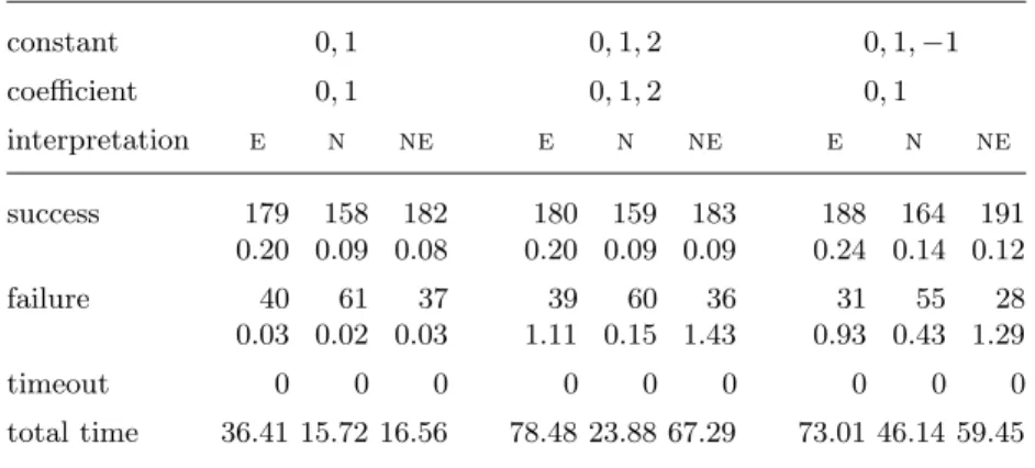
Tables 1 and 2 show the effect of the negative constant method developed in Section 3. In Table 1 we prove termination whereas in Table 1 we prove innermost termination. In the columns labelled n we use the natural interpretation for certain function symbols that appear in many example TRSs:
0Z= 0 1Z= 1 2Z= 2 · · ·
sZ(x) = x + 1 +Z(x, y) = x + y ×Z(x, y) = xy
pZ(x) = x − 11 −Z(x, y) = x − y1
For other function symbols we take linear interpretations fZ(x1, . . . , xn) = a1x1+ · · · + anxn+ b
1 In Tables 1 and 2 we do not fix the interpretation of p when −1 is not included in
Table 1.Negative constants: termination. constant 0, 1 0, 1, 2 0, 1, −1 coefficient 0, 1 0, 1, 2 0, 1 interpretation e n ne e n ne e n ne success 179 158 182 180 159 183 188 164 191 0.20 0.09 0.08 0.20 0.09 0.09 0.24 0.14 0.12 failure 40 61 37 39 60 36 31 55 28 0.03 0.02 0.03 1.11 0.15 1.43 0.93 0.43 1.29 timeout 0 0 0 0 0 0 0 0 0 total time 36.41 15.72 16.56 78.48 23.88 67.29 73.01 46.14 59.45
with a1, . . . , an in the indicated coefficient range and b in the indicated constant
range. In the columns labelled e we do not fix the interpretations in advance; for all function symbols we search for an appropriate linear interpretation. In the columns labelled ne we start with the default natural interpretations but allow other linear interpretations if (innermost) termination cannot be proved. Deter-mining appropriate coefficients can be done by a straightforward but inefficient “generate and test” algorithm. We implemented a more involved algorithm in our termination tool, but we anticipate that the recent techniques described in [6] might be useful to optimize the search for coefficients.
We list the number of successful termination attempts, the number of failures (which means that no termination proof was found while fully exploring the search space implied by the options), and the number of timeouts, which we set to 30 seconds. The figures below the number of successes and failures indicate the average time in seconds.
By using coefficients from {0, 1, 2} very few additional examples can be han-dled. For termination the only difference is [2, Example 3.18] which contains a unary function double that requires 2x as interpretation. The effect of allowing −1 as constant is more apparent. Taking default natural interpretations for cer-tain common function symbols reduces the execution time considerably but also reduces the termination proving power. However, the ne columns clearly show that fixing natural interpretations initially but allowing different interpretations later is a very useful idea.
In Table 3 we use the negative coefficient method developed in Section 4. Not surprisingly, this method is more suited for proving innermost termination because the method is incompatible with the recent modular refinements of the dependency pair method when proving termination (for non-overlapping TRSs). Comparing the first (last) three columns in Table 3 with the last three columns in Table 1 (Table 2) one might be tempted to conclude that the approach developed in Section 4 is useless in practice. We note however that several
chal-Table 2.Negative constants: innermost termination. constant 0, 1 0, 1, 2 0, 1, −1 coefficient 0, 1 0, 1, 2 0, 1 interpretation e n ne e n ne e n ne success 200 177 202 202 179 204 209 183 211 0.19 0.10 0.09 0.19 0.10 0.09 0.23 0.14 0.12 failure 39 62 37 37 60 35 30 56 28 0.04 0.03 0.05 1.19 0.16 1.47 0.92 0.43 1.26 timeout 0 0 0 0 0 0 0 0 0 total time 39.46 18.92 19.59 81.94 26.97 70.07 75.24 49.10 61.24
Table 3.Negative coefficients.
termination innermost termination interpretation e n ne e n ne success 109 102 114 181 161 185 0.74 0.39 0.58 0.04 0.06 0.07 failure 71 96 66 30 62 28 2.50 0.71 2.48 1.72 0.33 2.00 timeout 39 21 39 28 16 26 total time 1428.41 738.16 1400.60 899.01 511.14 848.25
lenging examples can only be handled by polynomial interpretations with nega-tive coefficients. We mention TRSs that are (innermost) terminating because of non-linearity (e.g. [2, Examples 3.46, 4.12, 4.25]) and TRSs that are terminating because the difference of certain arguments decreases (e.g. [2, Example 4.30]).
References
1. T. Arts and J. Giesl. Termination of term rewriting using dependency pairs. The-oretical Computer Science, 236:133–178, 2000.
2. T. Arts and J. Giesl. A collection of examples for termination of term rewriting using dependency pairs. Technical Report AIB-2001-09, RWTH Aachen, 2001. 3. F. Baader and T. Nipkow. Term Rewriting and All That. Cambridge University
4. A. Ben Cherifa and P. Lescanne. Termination of rewriting systems by polynomial interpretations and its implementation. Science of Computer Programming, 9:137– 159, 1987.
5. E. Contejean, C. March´e, B. Monate, and X. Urbain. CiME version 2, 2000. Available at http://cime.lri.fr/.
6. E. Contejean, C. March´e, A.-P. Tom´as, and X. Urbain. Mechanically proving termination using polynomial interpretations. Research Report 1382, LRI, 2004. 7. N. Dershowitz. 33 Examples of termination. In French Spring School of Theoretical
Computer Science, volume 909 of LNCS, pages 16–26, 1995.
8. N. Dershowitz and C. Hoot. Natural termination. Theoretical Computer Science, 142(2):179–207, 1995.
9. J. Giesl. Generating polynomial orderings for termination proofs. In Proc. 6th RTA, volume 914 of LNCS, pages 426–431, 1995.
10. J. Giesl, T. Arts, and E. Ohlebusch. Modular termination proofs for rewriting using dependency pairs. Journal of Symbolic Computation, 34(1):21–58, 2002. 11. J. Giesl, R. Thiemann, P. Schneider-Kamp, and S. Falke. Automated termination
proofs with AProVE. In Proc. 15th RTA, volume 3091 of LNCS, pages 210–220, 2004.
12. N. Hirokawa and A. Middeldorp. Automating the dependency pair method. In Proc. 19th CADE, volume 2741 of LNAI, pages 32–46, 2003.
13. N. Hirokawa and A. Middeldorp. Dependency pairs revisited. In Proc. 16th RTA, volume 3091 of LNCS, pages 249–268, 2004.
14. N. Hirokawa and A. Middeldorp. Tyrolean termination tool. In Proc. 7th Interna-tion Workshop on TerminaInterna-tion, Technical Report AIB-2004-07, RWTH Aachen, pages 59–62, 2004.
15. H. Hong and D. Jakuˇs. Testing positiveness of polynomials. Journal of Automated Reasoning, 21:23–28, 1998.
16. D. Lankford. On proving term rewriting systems are Noetherian. Technical Report MTP-3, Louisiana Technical University, Ruston, LA, USA, 1979.
17. S. Lucas. Polynomials for proving termination of context-sensitive rewriting. In Proc. 7th FoSSaCS, volume 2987 of LNCS, pages 318–332, 2004.
18. S. Lucas. Polynomials over the reals in proof of termination. In Proc. 7th Interna-tion Workshop on TerminaInterna-tion, Technical Report AIB-2004-07, RWTH Aachen, pages 39–42, 2004.
19. J. Steinbach. Generating polynomial orderings. Information Processing Letters, 49:85–93, 1994.
20. J. Steinbach and U. K¨uhler. Check your ordering – termination proofs and open problems. Technical Report SR-90-25, Universit¨at Kaiserslautern, 1990.
21. Terese. Term Rewriting Systems, volume 55 of Cambridge Tracts in Theoretical Computer Science. Cambridge University Press, 2003.
22. R. Thiemann, J. Giesl, and P. Schneider-Kamp. Improved modular termination proofs using dependency pairs. In Proc. 2nd IJCAR, volume 3097 of LNAI, pages 75–90, 2004.
23. X. Urbain. Modular & incremental automated termination proofs. Journal of Automated Reasoning, 2004. To appear.
24. H. Zantema. Termination of term rewriting by semantic labelling. Fundamenta Informaticae, 24:89–105, 1995.