On the connection formula for the first Painleve equation : from the viewpoint of the exact WKB analysis(Painleve Transcendents and Asymptotic Analysis)

On

the

connection

formula

for the first

Painlev\’e

equation

–from

the

viewpoint

_of

the

exact

$WKB$

analysis

_–.

Yoshitsugu

TAKEI

Research Institute for Mathematical

Sciences

Kyoto University Kyoto, 606-01,

JAPAN

(

京油田裡厨

竹痔義次

)

1

Introduction.

In the workshop (held at the Research Institute for Mathematical Sciences,

Kyoto University during the period of April 26–28, 1995) I gave aseries of

lectures on the exact WKB analysis ofPainlev\’e transcendentswith a large parameter, the subject of my recent research jointly done with T. Kawai

(RIMS,Kyoto Univ.) and T.Aoki (Kinki Univ.). Startingwiththeexistence

offormal power series solutions $\lambda_{J}$ ofthe J-thPainlev\’e equation $(P_{J})(J=$

I,

.. .

, VI) and the definition ofturning points and Stokes curves for them, I explained the following topics mainly in my lectures:

1. local equivalence between $\lambda_{\mathrm{I}}$ and $\lambda_{J}(J=\mathrm{I}\mathrm{I}, \ldots, \mathrm{V}\mathrm{I})$,

2. construction ofinstanton-type formal solutions $\lambda_{J,\alpha,\beta}$ of $(P_{J})$,

3. descriptionoftheconnection formula for $\lambda_{\mathrm{I}}$ in terms of the

instanton-type solutions $\lambda_{\mathrm{I},\alpha,\beta}$,

4. local equivalence between $\lambda_{\mathrm{I},\alpha,\beta}$and $\lambda_{\mathrm{I}\mathrm{I},\alpha,\beta}$

.

The formal power series solutions $\lambda_{J}$ and, in particular, their local

equiva-lence are discussed in [KT2] in detail, while the readers should be referred

concentrate our consideration on the topic 3, i.e., on theconnection formula for the first Painlev\’e equation.

There have beenseveralworksabout theconnection formula for the first

Painlev\’e equation. For example, some Russian mathematicians investigate

Painlev\’e equations by using their relationship with the isomonodromic de-formations of linear equations associated with them. (See e.g. [FIK], and references cited there.) In particular, Kapaev has performed asymptotic

analysis ofthe associatedlinear equation to obtain theleading coefficient of

the connection formula for the first Painlev\’e equation $([\mathrm{K}])$

.

On the other

hand, employing the so-called multiple-scale analysis, Joshi and Kruskal

study the first (and the second) Painlev\’e equation without resorting to the isomonodromic method $([\mathrm{J}\mathrm{K}1, \mathrm{J}\mathrm{K}2])$

.

..

Now the purpose of our research is to discuss the Painlev\’e equation

$(P_{J})$ in a unified manner through the exact WKB analysis (cf. [Tke]). As

a matter offact, as is shown by the local equivalence between $\lambda_{\mathrm{I}}$ and $\lambda_{J}$,

the first Painlev\’e equation $(P_{\mathrm{I}})$ can be regarded as a canonical equation

near a simple turning point of $(P_{J})$ from the viewpoint of the exact WKB

analysis(just like the Airyequationin thecaseoflinear ordinarydifferential equations of second order). This, being one of the supporting evidences for

the possibility of such a unified treatment of $(P_{J})$, implies that explicit

analysis of$(P_{\mathrm{I}})$ should be a crucially important step for the determination

oftheconnectionformula for$(P_{J})$ nearasimpleturning point. Todetermine

the explicit form ofthe connection formula for $(P_{\mathrm{I}})$, we shall compute the

Stokes multipliers of the linear equation associated with $P_{\mathrm{I}}$ by using the

exact WKB analysis; to be more specific, we shall employ not only the Voros theory $([\mathrm{V}])$ but also Kapaev’s idea$(1\mathrm{K}])$ to overcomethe difficulty of

the double turning point whose appearance is a characteristic phenomenon

in our theory (cf. [KT1, $\mathrm{K}\mathrm{T}2]$). At the present stage the results we have

obtained so far are not satisfactory enough (in the sense that the explicit

formulas are obtained only for the leading term, not for arbitrarily higher

orders), althoughwe hope our method will giveus a complete answer in the near future.

By the way, we also note the following fact here; the number of the formal power series solutions $\lambda_{J}$ is exactly equal to the numberof the local

charts, which are constructed explicitly by Takano et al., of ‘the space of initial values for $(P_{J})$’ (due to Okamoto, cf. [Tka]). As I mentioned at the

end of the lectures, ourdream (just a dream in the true sense) is that this coincidence is not accidentalat all but may be akey property in considering

also that this dream will be realized in some future.

In ending this introduction, the author would like to thank Professor

T. Kawai and ProfessorT. _{Aoki for their many valuable suggestions and the}

stimulating discussions withthem. A partof thiswork waspreparedduring the author’s stay at the Isaac Newton Institute for Mathematical Sciences

supported by the joint research project ($‘ \mathrm{I}\mathrm{n}\mathrm{f}\mathrm{i}\mathrm{n}\mathrm{i}\mathrm{t}\mathrm{e}$ Analysis

and Geometry”

between the Newton Institute and RIMS, which is sponsored by the Royal Society and the Japan Society for the Promotion of Science.

2

Basic

part of the

exact

WKB

analysis

for

$(P_{\mathrm{I}})$

.

–A brief

review.

First ofall, to fix our notations, let us review the basic part of the exact WKB analysis for the first Painlev\’e equation.

The concrete form of the equation is given by the following:

(1) $\frac{d^{2}\lambda}{dt^{2}}=\eta^{22}(6\lambda+t)$,

which is equivalent to the following Hamiltonian system:

(2) $\{$

$\frac{d\lambda}{dt}$

$=$ $\eta\frac{\partial I\mathrm{f}_{\mathrm{I}}}{\partial\nu}$, $\frac{d\nu}{dt}$

$=$ $- \eta\frac{\partial IC_{\mathrm{I}}}{\partial\lambda}$,

where $IC_{\mathrm{I}}=\nu^{2}/2-(2\lambda^{3}+t\lambda)$

.

Here and in what follows

$\eta$ denotes a large

parameter. We also denote the polynomial $6\lambda^{2}+t$ by $F_{\mathrm{I}}(\lambda, t)$

.

As is

well-known,the equation (1) (or rather thesystem (2)) represents _{the condition}

for isomonodromic deformations of the following Schr\"odinger equation in

the

sense

of [JMU] (see [O] and [KT2] also):

(3) $(- \frac{\partial^{2}}{\partial x^{2}}+\eta^{2}Q_{\mathrm{I}}(X, t, \eta).)\psi(x, \iota, \eta)=0$,

where the potential $Q_{\mathrm{I}}$ is given by

Observing this concrete form of the equation, we can easily find that the system (2) (hence the equation (1) also) has the $\mathrm{f}\mathrm{o}\mathrm{l}1_{0}\mathrm{w}\mathrm{i}\mathrm{n}\mathrm{g}\mathrm{f}-1\mathrm{o}\mathrm{r}\mathrm{m}\mathrm{a}1$power series solution, which is denoted by $(\lambda_{\mathrm{I}}, \nu_{\mathrm{I}})$, with respect to

$\eta$ :

(5) $\{$

$\lambda_{1}$ $=$ $\lambda_{0}(\iota)+\eta-1\lambda_{1}(t)+\eta-2\lambda_{2}(t)+\cdots$ ,

$\nu_{1}$ $=$ $\nu_{0}(t)+\eta-1\nu_{1}(t)+\eta-2\nu_{2}(t)+\cdots$

.

An important point is that the requirement $(\lambda_{1}, \nu_{\mathrm{I}})$ should be a solutionof

(2) forces its leading term $(\lambda 0, \nu_{0})$ to satisfy the algebraic equations

(6) $F_{\mathrm{I}}(\lambda \mathrm{o}(t),t)=0$ and $\nu_{0}(t)=0$

and also the other terms $(\lambda_{j}, \nu_{j})(j\geq 1)$ to be determined recursively from

$(\lambda_{0}, \nu_{0})$

.

In particular, for $\lambda_{\mathrm{I}}$ the odd order terms all vanish identically and

everyeven order termcan be expressed in the following way:

(7) $\lambda_{2j}=c_{j}(-\frac{t}{6})^{(5j)/2}1-$ _{$(j=0,1,2, \cdots)$},

where $\{c_{j}\}$ is a series of constants defined by

(8) $\{$

$c_{0}$ $=$ 1, $c_{1}=- \frac{1}{12^{3}}$, $c_{2}=- \frac{49}{2\cdot 12^{6}}$,

$c_{j}$ $=$

$\frac{25}{12^{3}}(j-1)2c_{j}-1-\frac{1}{2}k,l+l_{-,\geq}-j\sum_{k}2c_{k}c_{l}$

$(j\geq 3)$

.

(Similarly all of the odd orderterms $\mathrm{i}\mathrm{d}\mathrm{e}\mathrm{n}\mathrm{t}\mathrm{i}_{\mathrm{C}}\mathrm{a}\mathrm{l}\mathrm{i}\mathrm{y}$vanish for

$\nu_{\mathrm{I}}.$) As is always

the case with singular perturbations, the recursive formula (8) makes $\lambda_{\mathrm{I}}$

diverge. To give an analytic meaning to $\lambda_{\mathrm{I}}$, we

consider.

its Borel sum, which is the central object ofour discussion in this report.

In [KT2] we have defined the turning points and the Stokes curves for formal power series solutions of$(P_{J})$

.

In thecaseof the equatin (1), i.e., the

first Painlev\’e equation, the origin $t=0$ is the unique turning point (which

is simple) and the Stokes curves become the following:

(9) $\{t\in C;{\rm Im}\int^{t}0\sqrt{\frac{\partial F_{\mathrm{I}}}{\partial\lambda}(\lambda_{0}(t),\iota)}dt=0\}$ ,

namely$\{t\in C;{\rm Im}(-t)5/4\}=0$, five straightlinesemanating fromtheorigin. Note that the turning points and theStokescurvesfor$\lambda_{\mathrm{I}}$ thusdefined havea

close relationship with those of the associated Schr\"odinger equation (3)$-(4)$ (see Proposition 1 in

\S 4.1

below). This relationship (and, in the case of the first Painlev\’e equation, the concrete analysis of the Borel transform of $\lambda_{\mathrm{I}}$

to be done in the subsequent section as well) explains the reason why the Borelsum of$\lambda_{\mathrm{I}}$ isexpected to have a discontinuityon the Stokes curves, as we shall see later.

Our goal in this report is to present, as explicitly as possible, the

con-nection formula describing the discontinuity of the Borel sum of $\lambda_{\mathrm{I}}$ on a

Stokes curve. Recalling the definition of the Borel resummation, we may

easily guess that the connection formula should be described in terms of

the ‘instanton-type’ solutions introduced in [KT1] first. As a matter of fact, in [AKT3] we have constructed the following formal solutions $\lambda_{\mathrm{I},\alpha,\beta}$ of

the equation (1) with two free parameters by employing the multiple-scale analysis:

(10) $\lambda_{\mathrm{I},\alpha,\beta}=\lambda 0(t)+\eta\lambda_{1}-1/2-+\eta 1/2(t, \eta)\lambda 1(t, \eta)+\cdots$,

where the leading term $\lambda_{0}(t)$ is the same as that of $\lambda_{\mathrm{I}}$, i.e., $\lambda_{0}(t)=s^{1/2}$

$(s=-t/6)$, the sub-leading term $\lambda_{1/2}(t, \eta)$ is given by

(11) $\lambda_{1/2}(t, \eta)=(12\lambda 0)^{-1}/4[\alpha \mathit{8}^{5\alpha\beta}/2e^{\mathcal{T}}+\beta S^{-5\alpha\beta/\tau}2e^{-}]$

with $\alpha$ and $\beta$ being arbitrary complex numbers and

(12) $\tau=\eta\int_{0}^{t}\sqrt{\frac{\partial F_{\mathrm{I}}}{\partial\lambda}(\lambda_{0}(t),t)}dt=-\frac{48\sqrt{3}}{5}(-\frac{t}{6})^{5}/4\eta$,

and the higher order terms $\lambda_{j/2}(t, \eta)(j\geq 2)$, which are determined

recur-sively from $\lambda_{0}(t)$ and $\lambda_{1/2}(t, \eta)$, have the following form:

(13) $\lambda_{j/2}(t, \eta)=\sum_{=k0}^{j}\lambda_{j}^{(j}/2)e-2k(\iota)(j-2k)_{\mathcal{T}}$

.

Remark. Although it is possible to introduce more arbitrary constants into the formal solution $\lambda_{\mathrm{I},\alpha,\beta}$ in determining _{$\lambda 2((2\iota_{-}1)/t, \eta)$} for every

pos-itive integer $l$, we assume throught this report that all of them are zero

except $(\alpha, \beta)$ contained in the expression (11) of$\lambda_{1/2}(t, \eta)$

.

In fact, for our

purposes it is sufficientto consider such a simple case due to the distinctive homogeneity (with respect to $t$ and

$\eta$) that the solution

equation (1) enjoys. For the details concerning these solutions see [AKT3,

\S 1],

where the other Painlev\’e equations are also discussed.

Furthermore, if we assume one of the free parameters, say $\beta$, to be zero,

thenwe find that the ‘negative instanton-terms’ (i.e., the terms $\lambda(t)e^{(j-}2k$)$\tau$

with$j-2k<0$ in the expression (13)of$\lambda_{j/2}(t, \eta))$ allvanish and the formal

solution $\lambda_{\mathrm{I},\alpha,0}$ can beexpressed in another way, namely

(14) $\lambda_{\mathrm{I},\alpha_{:}}0$

. $=\lambda(0)+\eta^{-1}\lambda/2(1)e+\mathcal{T}\eta\lambda 2)e+-1(2\mathcal{T}\ldots$ ,

where each $\lambda^{(j)}=\sum_{k\geq 0}\eta^{-k}\lambda_{j}^{(+}/2$$(t)kj$) is a formal power series of$\eta^{-1}$

.

In

particular, $\lambda^{(0)}$ coincides with the formal power series solution $\lambda_{\mathrm{I}},$ $\lambda^{(1)}$

has the form

(15) $\lambda^{(1)}=\alpha(12\sqrt{s})^{-1/4}[1-\frac{15}{4}(12\sqrt{s})^{-5/1]}2\eta+-\ldots$,

and the other $\lambda^{(j)}(j\geq 2)$ are determined recursively. (A similar expression

is possible also for $\lambda_{\mathrm{I},0,\beta}.$) This particular solution $\lambda_{\mathrm{I},\alpha,0}$ (or $\lambda_{\mathrm{I},0,\beta}$), which

is nothing but the solution discussed in $[\mathrm{K}\mathrm{T}1, \S 3]$, should be an important

ingredient of theconnectionformula for$\lambda_{\mathrm{I}}$

.

Inthesequelwetryto determine

the explicit form (or, equivalently, the explicit value of the constant $\alpha$ (or

$\beta))$ of the solution that appears in the connection formula for $\lambda_{\mathrm{I}}$

.

3

Analytical

structure

of the Borel transform and

the

connection

formula for

$\lambda_{\mathrm{I}}$

.

Before discussing the Stokes multipliers of the linear equation (3)$-(4)$, we

investigate some analytical properties ofthe Borel transform of $\lambda_{\mathrm{I}}$ without

applying the isomonodromic method. The content of this section is

essen-tially the same as that of$[\mathrm{K}\mathrm{T}1, \S 3]$

.

Let $\lambda_{\mathrm{I},B}(t, y)$ denote the Borel transform of $\lambda_{\mathrm{I}}$

.

Since the Borel sum of $\lambda_{\mathrm{I}}$ is defined as a Laplace integral

$\eta\int_{0}^{\infty}e^{-y\eta}\lambda_{\mathrm{I}},B(t, y)dy$,

it is reasonable to guess that the Borel sum of $\lambda_{\mathrm{I}}$ may have a discontinuity

we denote by $\phi(t_{*})$, lies on the positive real axis and that it should satisfy

the followingconnection formula there:

(16) $\lambda_{\mathrm{I}}arrow\lambda_{\mathrm{I}}+e^{-\phi(t)\eta}\tilde{\lambda}+\cdot$

.

,

.

Here $\tilde{\lambda}$

corresponds to (the Borel sum of) the singular part of $\lambda_{\mathrm{I},B}(t, y)$

at the singular point $y=\phi(t)$

.

(In (16) we use the same symbol $\lambda_{\mathrm{I}}$ to

designate its Borel sum also.) Inthis mannerthe analytical structure of the

Borel transform$\lambda_{\mathrm{I},B}$ (i.e., thelocation of its singular points andits singular

part at every singular point) completelydetermines the explicit form of the connection formula for $\lambda_{\mathrm{I}}$

.

On the other hand, we find that the right-hand side of (16) has the

same form as that of one parameter _{instanton-type solutions defined by}

(14). As a matter of fact, it must be one of the instanton-type solutions

due to the “uniqueness” of this kind of solutions ($[\mathrm{K}\mathrm{T}1$, Theorem 3.1]) and

to the homogeneity of $\lambda_{\mathrm{I}}$

.

This implies, under the assumption of the Borel

summability of$\lambda_{\mathrm{I}}$, that the explicit description of instanton-type solutions

explained in

\S 2

should be translated into the corresponding information on the analytical structure of $\lambda_{\mathrm{I},B}$ and as a consequence the connection

formula for$\lambda_{\mathrm{I}}$ should bedetermined completelyexceptoneconstant

$\alpha$ which

is contained in the expression (14)$-(15)$ of one _parameter instanton-type

solutions.

From now on let us investigate theanalytical structure of $\lambda_{\mathrm{I},B}$ by using

its relationshipwiththe explicit_{description of instanton-type solutions and}

try to fix the undetermined constant $\alpha$ mentioned above. By the definition

the explicit form of$\lambda_{\mathrm{I},B}$ is the following:

(17) $\lambda_{\mathrm{I},B}(t, y)=\sum_{j=0}\frac{c_{j}}{(2j)!}\infty(-\frac{t}{6}\mathrm{I}^{(1-\mathrm{s}}j)/2y^{2j}$,

where the coefficient $c_{j}$ has already been defined by (8). Taking the

homo-geneity of$\lambda_{\mathrm{I}}$ and

$\lambda_{\mathrm{I},B}$ into account, werewrite (17) as follows:

(18) $\lambda_{\mathrm{I},B}(t, y)=(-\frac{t}{6})^{1}/\sum_{j=0}^{2\infty}d_{j}zj$,

where

It follows from the recursive formula (8) that the series $\{d_{j}\}$ satisfies, for

example, the following estimate:

(20) $C4^{j} \frac{(j-1)!^{2}}{(2j)!}\leq|d_{j}|\leq 4^{j+1}\frac{j!^{2}}{(2j+2)!}$ $(j\geq 1)$

where $C$ is a positive constant. By using this estimate (20) we can readily

verify that the sum $\sum d_{j}z^{j}$ converges for small $z$ and that its radius of

convergenceis equal to 1. Furthermore, since $d_{j}$ is negative for every$j\geq 1$,

the point $z=1$ is a singular point of $\sum d_{j}z^{j}$

.

This immediately implies

that for each fixed $t\neq 0$ the Borel transform $\lambda_{\mathrm{I},B}(t, y)$ defines an analytic

function near $y=0$ and has a singularity at $y= \pm\frac{48\sqrt{3}}{5}(-t/6)5/4$ which

is denoted by $\pm\phi_{\mathrm{I}}(t)$ hereinafter. The location of this singularity exactly

coincides (except the sign) with the one predicted by the explicit form of

instanton-type solutions (14) (cf. (12)). As the singular part of $\lambda_{\mathrm{I},B}(t, y)$

at this singular point $y=\phi_{\mathrm{I}}(t)$ corresponds to the coefficient $\eta^{-1/2}\lambda^{(}1$) of $e^{\tau}=e^{-\phi_{1}(t)}\eta$ in the expression (14), we canfurther expect that the function $\sum d_{j}z^{j}$ should have the following local expression near the singular point

$z=1$:

(21) $\sum d_{j}z^{j}=(1-Z)^{1}/2f(Z)+\mathit{9}(z)$

where $f$ and $g$ are holomorphic functions in a neighborhood of$z=1$

.

As

a matter of fact, $(1 -z)^{1/2}f(Z)$ _(or, more _{precisely, the discontinuity of} $(-t/6)^{1/2}(1-z)^{1/2}f(z))$ corresponds to the Borel transform of $\eta^{-1/2}\lambda^{(1)}$

.

(The term $(1-z)1/2$ essentiallycomes from $\eta^{-1/2}.$) In particular, it follows

from this correspondence that the undetermined constant $\alpha$ in the

connec-tion formula for $\lambda_{\mathrm{I}}$ is connected with the value of $f(z)$ at $z=1$ by the

relation $\alpha=i\sqrt{5\pi}/12\mu(\mu=f(z)|_{z=}1)$

.

(Note that, strictly speaking, this

relation is correct except the sign. The sign may depend not only on the

choiceof various branches butalsoon which Stokescurves we areconsidering

at.)

Thus our remaining task is to fix the value $\mu=f(1)$

.

Let us recall

that the exponent $j\tau/\eta$ of “instantons” $e^{j\tau}$

in (14) represents the location ofsingular points of$\lambda_{\mathrm{I},B}(t, y)$

.

On the other hand, it follows from (12) that

the possible value of$j\tau/\eta$isonly anintegral multipleof$\phi_{\mathrm{I}}(t)$

.

This strongly

suggests that the point $z=1$ should be the uniquesingular pointof $\sum d_{j}z^{j}$

on its circle of convergence. Let us now assume this fact for the moment.

Then it enables us to apply the Darboux method to the analytic function

$z=1$ (hence $f_{0}=\mu$) and consider the function

$F_{N}(_{Z})= \sum_{j=0}d_{j}z-\infty j(1-Z)1/2k\sum_{=0}^{N-1}fk(Z-1)^{k}$

for a positive integer $N$

.

It follows from the above assumption and the

expression (21) that the holomorphic function $F_{N}(z)$ in $\{z\in C;|z|<1\}$

defines an $N$-times continuously differentiable function on the unit circle $\{z\in C;|z|=1\}$

.

Hence the coefficient of the Taylor expansionof $F_{N}(z)$ at

$z=0$, which is explicitly given by

$d_{j}- \sum_{k=0}^{N-1}(-1)j+kf_{k^{\frac{\Gamma(k+3/2)}{j!\Gamma(k+3/2-j)}}}$,

becomes $O(j^{-M})$ for an arbitrarily given _{positive number} $M$ providing $N$

is sufficiently large, as it is at the same time the Fourier coefficient of the

$2\pi$-periodic $C^{N}$ function $F_{N}(e^{i\theta})$

.

Since $(j!\Gamma(k+3/2-j))^{-1}=O(j^{-k-}3/2)$

holds for every non-negative integer $k$, this immediately implies

(22) $\mu=f_{0}=\lim_{jarrow\infty}(-1)^{j}d_{j}\frac{j!\Gamma(3/2-j)}{\Gamma(3/2)}$

.

Combining(22)andtherecursive formula for$\{d_{j}\}$ (cf. (8) and(19))together,

we thus obtain the followingexpression of$\mu$:

(23) $\mu=\lim_{jarrow\infty}\mu j$

with $\{\mu_{j}\}$ being defined by the following:

(24) $\{$

$\mu_{0}$ $=$ 1, $\mu_{1}=\frac{4}{25}$ $\mu_{2}=\frac{392}{1875}$

$\mu_{j}$ $–$ $\frac{(2j-2)^{2}}{(2j-1)(2j-3)}\mu_{j-1}$

$+ \frac{1}{2}\sum\frac{(2k-1)!!(2k-3)!!(2l-1)!!(2l-3)!!}{(2j-1)!!(2j-3)!!}\mu_{k}\mu_{l}$

$k+l^{--j}k,l\geq 2$

$(j\geq 3)$

(where $(2n-1)!!=(2n-1)\cdot(2n-3)\cdots\cdot 1$). A numerical computation of

(23)$-(24)$ shows, for example,

(Note that for the numerical computation of$\mu$ it is better to use some error

estimate together since the convergence of (23)$-(24)$ is considerablyslow.)

The conclusion of this sectioncanbe summarized as follows: Thestudy

based on the relationship between the analytical structure of the Borel transform $\lambda_{\mathrm{I},B}$ and the explicit descriptionof instanton-type solutions tells

us that under several assumptions such as the Borel summability of $\lambda_{\mathrm{I}}$

etc. we have the following connection formula for $\lambda_{\mathrm{I}}$ on each Stokes curve

$\{t\in C;{\rm Im}(-t)^{5/4}=0\}$:

(26) $\lambda_{\mathrm{I}}$ $arrow$ $\lambda_{\mathrm{I},\alpha,0}$

$=$ $\lambda_{\mathrm{I}}+\eta\lambda-1/2(1)-e\phi 1(\iota)\eta+\eta\lambda-1(2)e-2\mathrm{I}(\iota)\eta+\emptyset\ldots$,

where

(27) $\phi_{\mathrm{I}}(t)$ $=$ $\frac{48\sqrt{3}}{5}s^{5/4}$ $(s=- \frac{t}{6})$,

(28) $\lambda^{(1)}$

$=$ $i \sqrt{\frac{5\pi}{12}}\mu(12\sqrt{s})^{-1/4}[1-\frac{15}{4}(12\sqrt{s})-5/2-1]\eta+\cdots$,

and the other $\lambda^{(j)}(j\geq 2)$ are determined recursively. (On some Stokes

curves

the formula (26) holds with $\lambda_{\mathrm{I},\alpha,0}$ being replaced by $\lambda_{\mathrm{I},0,\beta}.$) The

constant $\mu$ is the limit ofthe series $\{\mu_{j}\}$ defined by (24).

4

Isomonodromic

deformations of the associated

linear equation and the

connection

formula for

$\lambda_{\mathrm{I}}$

.

Inthe precedingsection wehavepresented a characterization ofthe undeter-mined constant and deterundeter-mined the explicitform ofthe connection formula for $\lambda_{\mathrm{I}}$ in a quite satisfactory manner. However we have to admit that the

exact valueofthe constant is still notfixed; we can compute it only

numer-ically. In this section we consider our problem by using the relationship of

the equation (1) with isomonodromic deformations of the associated linear equation (3)$-(4)$ and try again to fixthe constant explicitly.

4.1

Preliminaries.

First ofall, let us substitute

$(\lambda_{0}(t)=\sqrt{-t}/6)$ into the linear equation (3)$-(4)$

.

After the substitution the potential $Q_{\mathrm{I}}$ becomes the following:

(30) $Q_{\mathrm{I}}$ $=$ $4x^{3}+2tx-(4\lambda_{0}^{3}+2t\lambda_{0})+\eta^{-1}(N^{22}-12\lambda 0\Lambda)$

$- \eta^{-3/2}(4\Lambda^{3}+\frac{N}{x-\lambda_{0}}\mathrm{I}+\eta^{-2_{\frac{-N\Lambda+3/4}{(x-\lambda_{0})^{2}}+}}\cdots$

.

Now our strategy is as follows: We first compute a pair of two

inde-pendent Stokes multipliersofthe linear equation (3)$-(30)$ by employing the

exact WKB analysis due to Voros [V] (see [DDPI] and [AKT2] also). Since a double turning point naturally appears in our situation, we also make

use ofa local reduction theorem of [AKT3], based on Kapaev’s idea $([\mathrm{K}])$,

near the double turning point. As a consequence we will obtain an explicit description of the Stokes multipliers, which actually are infinite series of

$\eta^{-1/2}$ with their coefficients being functions of $t$, A and $N$

.

Then we solve

(

$‘ \mathrm{i}\mathrm{s}\mathrm{o}\mathrm{m}\mathrm{o}\mathrm{n}\mathrm{o}\mathrm{d}\mathrm{r}\mathrm{o}\mathrm{m}\mathrm{i}\mathrm{C}$ equations” (i.e., equations that require these Stokes

multi-pliers to beconstant) for A and$N$, regarding$t$ and

$\eta$ as parameters, to seek

solutions of the first Painlev\’e equation (1). If we perform this procedure

in two adjacent Stokes regions (i.e., sectorial regions surrounded by Stokes

curvesfor $\lambda_{\mathrm{I}}$) respectively, the connection formula for$\lambda_{\mathrm{I}}$ will be determined

explicitly. $\mathrm{W}$

Before starting the computation ofStokesmultipliers, let us make

some

important remarks concerningthe WKB-theoretic structure of the equation (3)$-(30)$ here.

First, since the top term $Q_{0}$ of $Q_{\mathrm{I}}$ is factorized as

$Q_{0}=4x^{3}+2tx-(4\lambda_{0}^{3}+2t\lambda_{0})=4(x-\sqrt{s})2(X+2\sqrt{s})$,

where $s$ denotes $-t/6$ as usual, the equation (3)$-(30)$ has a double turning

point at $x=\sqrt{s}$

.

This is really an unpleasant feature; the existence of

a double turning point prevents us from employing the Voros theory to

computethe Stokes

_mul.t

ipliers. Wewilldiscuss how to deal with this double turning point in the next subsection.

Second, in connection with this double turning point, the Stokes

geom-etry (i.e., the turning points and the Stokes curves) of the linear equation

(3)$-(30)$ is controlled by that of the Painlev\’e equation (1) in the following

manner:

Proposition 1 (i) At the turning point

_for

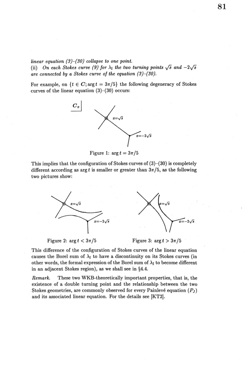
$\lambda_{\mathrm{I}}$ ($i.e.$, at $t=0$) the double

linear equation (3)$-(\mathit{3}\mathit{0})$ collapse to one point.

(ii) On each Stokes curve (9)

_for

$\lambda_{\mathrm{I}}$ the two turning points $\sqrt{s}and-2\sqrt{s}$

are connected by a Stokes curve

_of

the equation (3)$-(so)$

.

For example, on $\{t\in C;\arg t=3\pi/5\}$ the following degeneracy of Stokes

curves

of the linear equation (3)$-(30)$ occurs:

$\lrcorner C_{x}$

Figure 1: $\arg t=3\pi/5$

This implies that the configuration of Stokescurvesof(3)$-(30)$ is completely

different according as$\arg t$ is smaller or greater than $3\pi/5$, as the following

two pictures show:

Figure 2: $\arg t<3\pi/5$ Figure 3: $\arg t>3\pi/5$ This difference of the configuration of Stokes curves ofthe linear equation

causes the Borel sum of $\lambda_{\mathrm{I}}$ to have a discontinuity on its Stokes curves (in

other words,the formalexpressionof the Borelsumof$\lambda_{\mathrm{I}}$ to become different

in an adjacent Stokesregion), as we shall see in

_{\S 4.4.}

Remark. These two WKB-theoretically important properties, that is, the existence of a double turning point and the relationship between the two Stokes geometries, are commonlyobserved for everyPainlev\’e equation $(P_{J})$

4.2

Canonical

form

near

the double turning point.

In orderto compute theStokes multipliersof theequation (3)$-(30)$ we need

the connection formula for WKB solutions of(3)$-(30)$ on each Stokescurve

emanating from the double turning point $x=\sqrt{s}$

.

One problem is that the

point $x=\sqrt{s}$ is not only a double turning point but also a singular point

of (higherorder terms of) the potential (30). To overcome this difficultywe make use of a local transformation theorem (Proposition 2 below) near the double turning point, which is based on Kapaev’s idea $(1^{\mathrm{K}}])$ and proved in

all orders (with respect to $\eta^{-1/2}$) in [AKT3]. In this subsection we study

the canonical equation whichappears in this local transformation theorem. See also [DDP2] for a generaltreatment of double turning points.

Nowlet us first state the local transformation theorem.

Proposition 2 There exist a neighborhood $U$

of

$x=\sqrt{s}$, a

formal

series

(31) $\zeta(x, t, \eta)=j=\sum^{\infty}0\zeta_{j}/2(_{X}, t)\eta-j/2$,

whose

_coefficients

$\zeta_{j/2}(x, t)$ are holomorphic in $x\in U$ (and $al_{\mathit{8}}o$ in $t$), and

formal

series

(32) $E(t, \eta)$ $=$ _{$\sum_{j=0}^{\infty}E/2(ji)\eta^{-j}/2$},

(33) $\rho(t, \eta)$ $=$ $\sum_{j=0}^{\infty}\rho j/2(t)\eta^{-j}/2$,

so that the following

_four

conditions are

_satisfied:

(34) $\frac{\partial\zeta_{0}}{\partial x}$ nevervanishes,

(35) $\zeta_{0}(\sqrt{s}, t)=0$,

(36) $\zeta_{1/2}$identically vanishes,

(37) $Q_{\mathrm{I}}(x, t, \eta)=(\frac{\partial\zeta}{\partial x})^{2}[4\zeta(x, t, \eta)2+\eta^{-1}E(t, \eta)$

$+ \frac{\eta^{-3/2}\rho(t,\eta)}{\zeta(x,t,\eta)..-\zeta(\sqrt{s}+\eta^{-1/2}\Lambda,t,\eta)}$ $+ \frac{3\eta^{-2}}{4(\zeta(_{X},t,\eta)-\zeta(\sqrt{s}+\eta-1/2\Lambda,\iota,\eta))2}]$ $- \frac{1}{2}\eta^{-2}\{\zeta(x, t, \eta);x\}$,

where $\{\zeta;x\}$ denotes the Schwarzian derivative:

$\frac{\partial^{3}\zeta/\partial x^{3}}{\partial\zeta/\partial x}-\frac{3}{2}(\frac{\partial^{2}\zeta/\partial x^{2}}{\partial\zeta/\partial x})^{2}$

For the proof ofProposition 2we refer the reader to [AKT3]. In fact, itcan be verified inthe sameway as [AKT3, Theorem 3.1], although the situation is a little different in that here we assume only the relation (29) while in [AKT3] an instanton-type solution ofthe system (2) has already been sub-stituted into the potential $Q_{\mathrm{I}}$. Proposition 2 claims that in a neighborhood

of the double turning point $x=\sqrt{s}$the linear equation (3)$-(30)$ should be

transformed to the following canonical equation bythe transformation (31):

(38) $(- \frac{\partial^{2}}{\partial\zeta^{2}}+\eta^{2}Q\mathrm{c}\mathrm{a}\mathrm{n}(\zeta, t, \eta))\varphi(\zeta, t, \eta)=0$,

where

(39)$Q_{\mathrm{C}} \mathrm{a}\mathrm{n}=4\zeta 2E\eta^{-1}(+t, \eta)+\frac{\eta^{-3/2}\rho(t,\eta)}{\zeta-\eta^{-1/2}\sigma(t,\eta)}+\frac{3\eta^{-2}}{4(\zeta-\eta^{-1/2}\sigma(t,\eta))2}$

.

Here wehave denoted$\eta\zeta 1/2(\sqrt{s}+\eta^{-}1/2\Lambda, t, \eta)$by $\sigma(t, \eta)$ (whichis of order $0$

in $\eta$ by (35)$)$

.

Note that these formal power series$E(t, \eta),$

$\rho(t, \eta)$and$\sigma(t, \eta)$,

which depend also on A and $N$, are not independent; they satisfy

(40) $E(t, \eta)=\rho(t, \eta)^{2}-4\sigma(t, \eta)^{2}$

(cf. [AKT3, Remark3.3]). Furthermorethey aredetermined uniquely in the construction ofthe transformation. For example, the explicit form of their

top order terms is given by

(41) $E_{0}$ $=$ $(3\sqrt{s})^{-}1/2(N^{2}-12\sqrt{s}\Lambda^{2})$, (42) $\rho 0$ $=$ $-(3\sqrt{s})^{-1/4}N$,

(43) $\sigma_{0}$ $=$ $(3\sqrt{s})^{1/4}\Lambda$

.

In particular, the formal power series$E(t, \eta)$ is related to the original

equa-tion (3)$-(30)$ (and hence canbe computed easily) by the following relation:

(44) $E(t, \eta)=4{\rm Res}_{x=\sqrt{s}\circ}S\mathrm{d}\mathrm{d}$

(cf. [AKT3, (3.33)]), where $S_{\mathrm{o}\mathrm{d}\mathrm{d}}$ denotes the generalized odd part (in the sense of [AKT3, Definition 2.1]$)$ of the solution $S$ of the Riccati equation

associated with the original equation (3)$-(30)$, that is, $S_{\mathrm{o}\mathrm{d}\mathrm{d}}=(S^{+}-S-)/2$

with$S^{\pm}$ being thetwo

formal power series solutions of the Riccatiequation. In the rest ofthis subsectin we _{discuss the connection formula for WKB}

solutions of the canonical equation (38)$-(39)$

.

Let us denote the solution

of the associated Riccati equation by $T= \sum_{j\geq-2}\eta^{-j/2}\tau(j/2\zeta)$ and its

gen-eralized odd part by $T_{\mathrm{o}\mathrm{d}\mathrm{d};}$ for example, _{$\tau_{-1}=2\zeta$} and

$\tau_{-1/2}(\zeta)$ identically

vanishes. By the induction it can be readily verified that, for every $j\geq 0$,

$T_{j/2}(\zeta)$ contains terms with negative powers in $\zeta$ only and

(45) ${\rm Res}_{\zeta=}0T_{\mathrm{o}} \mathrm{d}\mathrm{d}={\rm Res}_{\zeta=0}(T_{\mathrm{o}\mathrm{d}\mathrm{d}}-\eta\tau_{-}1)=\frac{E(t,\eta)}{4}$

holds. Thus the following normalized WKB solutions of the equation

(38)-(39), which we use as a fundamentalsystem ofsolutions hereinafter, become well-defined:

(46) $\varphi\pm$ $=$ $\frac{\sqrt{2\eta}}{\sqrt{T_{\mathrm{o}\mathrm{d}\mathrm{d}}}}\zeta^{\pm E/4}$

$\cross\exp\pm\{\eta\int_{0}^{\zeta}\tau-1d\zeta+\int_{\infty}^{\zeta}(\tau_{\mathrm{o}\mathrm{d}\mathrm{d}}-\eta\tau_{-}1-\frac{E}{4\zeta})d\zeta\}$ ,

that is,

(47) $\varphi_{\pm}--\exp(\pm\eta\zeta 2)\zeta-1/2\pm E/4(1+O(\eta^{1}\zeta/2)-1)$

.

Note that the asymptotic behavior (47) uniquely determines the normaliza-tion of WKB solunormaliza-tions (in the formal sense). In what follows we consider

these WKB solutions $\varphi\pm \mathrm{i}\mathrm{n}$ the Stokes regions (Region I $\sim$ Region III)

indicated in Figure4.

Figure 4

(For ourpresent purposes, i.e., to determine the connection formula for $\lambda_{\mathrm{I}}$,

cutonthe negative imaginary axis and define a branchof$\zeta^{\pm E/4}$ etc. so that

$0<\arg\zeta<3\pi/2$ may be satisfied.

Now our task is to determine the connection formula for $\varphi\pm \mathrm{b}\mathrm{e}\mathrm{t}\mathrm{w}\mathrm{e}\mathrm{e}\mathrm{n}$

two adjacent regions ofRegion $\mathrm{I}\sim \mathrm{R}\mathrm{e}\mathrm{g}\mathrm{i}_{\mathrm{o}\mathrm{n}}$ III. To do so, we transform the

canonical equation (38)$-(39)$ into the Weber equation. As a matter of fact,

ifwe first define $\tilde{u}$ and $\tilde{v}$ by

(48) $\{$

$\tilde{v}$

$=$ $(\zeta-\eta^{-1}\sigma/2)^{1}/2\varphi$,

$\tilde{u}$ _$=$ $( \zeta-\eta^{-1/-1}2\sigma)\{\frac{d}{d\zeta}\tilde{v}+\eta^{1/2}\rho\tilde{v}\}$,

and if we, after that, apply the lineartransformation

(49)

$=$

,

we find

(50)

$\frac{d}{d\zeta}=\eta$

.

In particular, $u$ thus defined satisfies

(51) $\frac{d^{2}u}{d\zeta^{2}}=\eta^{2}(4\zeta 2\eta+-1(E+2))u$,

and the equation (51)

can

be transformed by the scaling $z=2\sqrt{\eta}\zeta$ ofthe

independent variable into the Weber equation:

(52) $\frac{d^{2}u}{dz^{2}}+(\kappa+\frac{1}{2}-\frac{z^{2}}{4}\mathrm{I}u=0$,

where $\kappa=-E/4-1$

.

In other words, if for a solution $\varphi$ of the canonical

equation (38)$-(39)$ we define $u(z)$ by

(53) $\varphi(\zeta)$ – $u(z)^{\mathrm{d}\mathrm{f}}=^{\mathrm{e}} \frac{\sqrt{2}\eta^{1/4}}{\sqrt{z-2\sigma}}[2\frac{d}{dz}(\varphi(\frac{z}{2\sqrt{\eta}}))$

then the resulting function $u(z)$ satisfies (52), and conversely (54) $u(z)$ $\mapsto$

$\varphi(\zeta)^{\mathrm{d}}=^{\mathrm{e}\mathrm{f}}\frac{1}{4\eta^{1/2}\sqrt{\zeta-\eta^{-1/2}\sigma}}$

$\cross[\frac{1}{\rho-2\sigma}(-2\frac{du}{dz}+zu)+u]|_{z=2\sqrt{\eta}\zeta}$

transforms asolution ofthe Weber equation (52) to a solution of(38)$-(39)$

.

Let us denote the former correspondence by $u=\mathcal{G}\varphi$ and the latter by $\varphi=\mathcal{G}^{-1}u$

.

Making use of this equivalence between the canonical equation

and the Weber equation, we compute the connection formula for $\varphi_{\pm}$ in the

following way:

It is well known that the Weber equation (52) has the following formal

solution denoted by$\overline{D_{\kappa}}(Z)$:

(55) $\overline{D_{\kappa}}(z)=e-z^{2}/4\kappa\sum^{\infty}Zn=0(-1)n_{\frac{\kappa(\kappa-1)\cdots(\kappa-2n+1)}{n!2^{n_{Z}2n}}}$

.

Similarly $\overline{D\kappa}(-Z)$ and $D_{\overline{-\kappa}-1}(\pm iz)$ also satisfy the equation. Now we pick

up two ofthem appropriately and regard them as afundamental system of solutions of (52) respectively in the Region $\mathrm{I}’\sim \mathrm{R}\mathrm{e}\mathrm{g}\mathrm{i}_{0}\mathrm{n}\mathrm{I}\mathrm{I}\mathrm{I}’$ in the complex

$z$-plane as is indicated below:

Here we choose a branch of$z^{\kappa}$ etc. so that the followingmay be satisfied in

each region:

$\{$

Region $\mathrm{I}’$ : $0<\arg z<\pi/2,$ $-\pi/2<\arg(-iz)<0$,

Region $\mathrm{I}\mathrm{I}’$: $-\pi/2<\arg(-Z)<0,0<\arg(-iz)<\pi/2$,

Region $\mathrm{I}\mathrm{I}\mathrm{I}’$ :

$0<\arg(-Z)<\pi/2,$ $-\pi/2<\arg(i_{Z})<0$

.

These formal solutions are important inthe sense that in every region they

correspond to the WKB solutions$\varphi\pm \mathrm{o}\mathrm{f}$the equation(38)$-(39)$ by the

trans-formation $\mathcal{G}$ defined $\dot{\mathrm{a}}$

bove. For example, a straightforward computation

shows that in Region $\mathrm{I}\ \mathrm{I}’$

(56) $\mathcal{G}^{-1}\overline{D_{\kappa}}(Z)=\frac{1}{\rho-2\sigma}(2\sqrt{\eta})^{\kappa}e^{-}\eta\zeta^{2}\zeta\kappa+1/2(1+o(\sqrt{\eta}\zeta)-1)$

.

This immediately implies

(57) $\mathcal{G}^{-1}\overline{D_{\kappa}}(z)=\frac{1}{\rho-2\sigma}(2\sqrt{\eta})^{\kappa}\varphi-=\frac{1}{\rho-2\sigma}(2\sqrt{\eta})^{-}E/4-1\varphi_{-}$

.

The other correspondences can be computed.in a similar manner (though it is necessary to pay some attention to the choice ofbranches). We write

down the complete list of them below:

(58) Region

I&I’

:

$\mathcal{G}^{-1}\overline{D_{\kappa}}(z)$

$=$ $\frac{1}{\rho-2\sigma}(2\sqrt{\eta})-E/4-1\varphi_{-}$, $\mathcal{G}^{-1}D_{-\hslash-}1(-iz)$ $=$ $\frac{1}{2}e^{-i\pi E/8}(2\sqrt{\eta})^{E/}4-1\varphi+$,

(59) Region

II&II’

:

$\mathcal{G}^{-1}\overline{D_{\kappa}}(-z)$ _{$=$ $- \frac{1}{\rho-2\sigma}e^{i\pi E//-}4(2\sqrt{\eta})-E41\varphi_{-}$},

$\mathcal{G}^{-1}D_{\overline{-\kappa}-}1(-iz)$ $=$ $\frac{1}{2}e^{-i\pi E/8}(2\sqrt{\eta})^{E/}4-1\varphi+$,

(60) Region

III&III’

:

. $\mathcal{G}^{-1}\overline{D_{\kappa}}(-z)$

.

$=$ $- \frac{1}{\rho-2\sigma}e^{i\pi E//-}4(2\sqrt{\eta})-E41\varphi_{-}$, $\mathcal{G}^{-1}D_{\overline{-\kappa}-1}(iZ)$ _$=$ $\frac{1}{2}e^{-3i\pi E/8}(2\sqrt{\eta})^{E/}4-1\varphi+\cdot$

On the other hand, according to the well-known asymptotic formula for the classical Weber function $D_{\kappa}(z)$ (cf. [BMP, Chapter 8.4]) we can

regard the Weber function $D_{\kappa}(z)$ (resp. $D_{\kappa}(-z)\underline{D}_{-\hslash-1},(\pm iz)$) as a Borel

sumoftheformal$\mathrm{s}\mathrm{o}\mathrm{l}\mathrm{u}\mathrm{t}\mathrm{i}_{0}\mathrm{n}\overline{D_{\kappa}}(Z)$(resp.$\overline{D_{\kappa}}(-Z),$ _{$D_{-}\kappa-1(\pm iz)$})ineachregion.

Furthermore, the well-known formulas (cf. [BMP, Chapter 8.2]) (61) $D_{\kappa}(z)$ $=$ $e^{i\pi\kappa}D_{\kappa}(-z)+ \frac{\sqrt{2\pi}}{\Gamma(-\kappa)}e^{i\pi(\kappa+}1)/2D-\kappa-1(-iz)$

(62) $D_{-\kappa-1}(-iz)$ $=$ $e^{-i\pi(\kappa+1)}D- \kappa-1(iZ)+\frac{\sqrt{2\pi}}{\Gamma(\kappa+1)}e^{-i\pi\kappa/}D_{\kappa}2(-z)$

for the Weberfunction $D_{\kappa}(z)$ then play a role ofthe connection formula for

theformal$\mathrm{s}\mathrm{o}\mathrm{l}\mathrm{u}\mathrm{t}\mathrm{i}_{0}\mathrm{n}\mathrm{s}\overline{D_{\kappa}}(z)$ etc. between

the $\mathrm{t}\mathrm{w}\underline{\mathrm{o}\mathrm{a}\mathrm{d}}\mathrm{j}\mathrm{a}\mathbb{C}\mathrm{e}\mathrm{n}\mathrm{t}$regions inquestion.

(Note that on the positive imaginary axis $D_{-\kappa-1}(-iz)$ is a subdominant

solution and so is $\overline{D_{\kappa}}(-Z)$ on the negative realaxis.)

Hence, combining the correspondences (58) $\sim(60)$ andthe classical

for-mulas (61)$-(62)$ together, we obtain the connection formula for the WKB

solutions$\varphi\pm \mathrm{o}\mathrm{f}$the canonicalequation (38)$-(39)$

.

Theresultis the following:

Proposition 3 Let $\varphi_{\pm}^{\mathrm{I}}$ (resp. $\varphi_{\pm}^{\mathrm{I}\mathrm{I}},$ $\varphi_{\pm}^{\mathrm{I}\mathrm{I}\mathrm{I}}$) denote the Borel sum

of

$\varphi\pm in$ the

Region I (resp. II, III) (cf. Figure 4). Then we have thefollowing relation:

(63) $\{$ $\varphi_{+}^{\mathrm{I}}$ _$=$ $\varphi_{+}^{\mathrm{I}1}$ $\varphi_{-}^{\mathrm{I}}$ $=$ $\varphi_{-+\frac{\rho-2\sigma}{2}\frac{\sqrt{2\pi}}{\Gamma(E/4+1)}}^{\mathrm{I}\mathrm{I}\pi E}e-i/4(2\sqrt{\eta})E/2\varphi_{+}^{\mathrm{I}\mathrm{I}}$, and (64) $\varphi_{+}^{\mathrm{I}\mathrm{I}}$ _$=$ $\varphi_{+}-\mathrm{I}\mathrm{I}\mathrm{I}\frac{2}{\rho-2\sigma}\frac{\sqrt{2\pi}}{\Gamma(-E/4)}e)/2(i\pi(E+12\sqrt{\eta})-E/2\varphi_{-}\mathrm{I}\mathrm{I}\mathrm{I}$ $\varphi_{-}^{\mathrm{I}\mathrm{I}}$ $=$ $\varphi_{-}^{\mathrm{I}\mathrm{I}\mathrm{I}}$

.

4.3 Computation of the Stokes multipliers.

Making use of the connection formula of the canonical equation near the double turningpoint, i.e., Proposition3 verifiedin the preceding subsection,

and the Voros theory $([\mathrm{V}])$ aswell, wecomputethe Stokes multipliersof the

linear equation associated with the firstPainlev\’eequationin this subsection. For the sake of specification, in otherwords, inorder to fix the configuration ofStokescurvesand thebranch of various multi-valued functions, we restrict

ourconsiderations heretoaneighborhood of the Stokescurve$\{t\in C;\arg t=$

$3\pi/5\}$ for $\lambda_{\mathrm{I}}$

.

The other cases can be discussed in the same way.

Now the equation we want to discuss is (3) with the potential $Q_{\mathrm{I}}$ given

by (30). To compute its Stokes multipliersweneedawell-normalizedformal

solution, which inoursituationcan be expressed in terms of WKB solutions

as follows:

(65) $\psi_{\pm}=\frac{\sqrt{2\eta}}{\sqrt{S_{\mathrm{o}\mathrm{d}\mathrm{d}}}}\exp\pm\{\eta\int_{-2\sqrt{s}}^{x}S_{-1}dX+\int_{\infty}^{x}(s_{\mathrm{o}\mathrm{d}\mathrm{d}\eta}-S-1)dx\}$ ,

where $S= \sum_{j>_{-}2}\eta^{-}s_{j/}2(j/2x)$ denotes the solution of the Riccati equation

associated $\mathrm{w}\mathrm{i}\mathrm{t}\overline{\mathrm{h}}(3)-(30)$and $S_{\mathrm{o}\mathrm{d}\mathrm{d}}$ designates its generalized odd part (cf.

[AKT3, Definition 3.1]$)$

.

For example, the top term $S_{-1}(x)$ is given by

$S_{-1}(x)=2(x-\sqrt{s})^{\sqrt{x+2\sqrt{s}}}$

$(s=-t/6)$ whose branch is determined so that $\arg S_{-}1(X)=\pi/5$ may

be satisfied on the segment connecting $x=\sqrt{s}$ and $x=-2\sqrt{s}$ (which is nothing but a Stokes curve of the equation (3)$-(30))$ when $\arg t=3\pi/5$

(i.e., $\arg s=8\pi/5$ and$\arg\sqrt{s}=4\pi/5$). Notethat $S_{-1/2}$ identicallyvanishes

and $S_{j/2}=O(x^{-3}/2)$ (as $xarrow\infty$) holds for every$j\geq 0$

.

Hence thesolutions

(65) are well-defined in the formal sense and, since

(66) $\int^{x}s_{-1(}X)dX$ $=$ 2$\int^{x}(x-\sqrt{s})(x+2\sqrt{s})1/2dx$

$=$ $\frac{2}{5}(x-3\sqrt{s})(X+2\sqrt{s})3/2$

holds (moduloconstants depending on$t$), theyhave thefollowingasymptotic

behavior as $xarrow\infty$:

(67) $\psi_{\pm}=x^{-3/4}\exp\{\pm\eta(\frac{2}{5}X5/2+\frac{t}{2}x^{1/2}\mathrm{I}\}(1+O(x^{-1/}2))$

.

Our next problem is to determine the connection formula for the nor-malized WKB solutions $\psi_{\pm}$ on a Stokes curve emanating from the double

turningpoint. We will solve this by using the local transformation between theequation (3)$-(30)$ inquestion and the canonicalequation (38)$-(39)$

pro-vided by Proposition 2. First let $\psi_{\pm}^{J}$ ($J=\mathrm{I},$ $\mathrm{I}\mathrm{I}$, III) denote the Borel sum

$\lrcorner C_{x}$

Figure 6: (A local picture near $x=\sqrt{s}.$)

Since the leading term (i.e., the geometric part) $\zeta_{0}(X, \iota)$ of the local

trans-formation (31) is definedby

(68) $\zeta_{0}(X, \iota)=(2\int_{\sqrt{s}}^{x}(x-\sqrt{s})(X+2\sqrt{s})^{1/2}dX)^{1}/2$ ,

$\lrcorner C_{x}$ $\llcorner C_{\zeta}$

$\zeta=\zeta_{0}(_{X}, t)$

Figure 7: Transformation$\zeta=\zeta_{0}(x, t)$

.

the Borel resummed WKB solution $\psi_{\pm}^{J}$ (_{$J=\mathrm{I},$}$\mathrm{I}\mathrm{I}$,

III) should correspond

to $\varphi_{\pm}^{J}$ respectively under the transformation (31). As a matter of fact, it

follows from (37) that$\psi_{\pm}$ and$\varphi\pm \mathrm{s}\mathrm{a}\mathrm{t}\mathrm{i}\mathrm{S}\mathrm{f}\mathrm{y}$thefollowing relation in the formal sense:

(69) $\psi_{\pm}(x, t, \eta)=C_{\pm}(t, \eta)(\frac{\partial\zeta}{\partial x})^{-1/2}\varphi_{\pm}(\zeta(x, t, \eta), t, \eta)$,

form:

(70) $C_{\pm}(t, \eta)=\exp(\eta c^{(\pm)}-1(t))\sum_{0}^{\infty}\eta c_{-j}j=)-j/2(\pm)/2(\iota$

.

Therelation (69) together with the geometric picture of the transformation

$\zeta=\zeta_{0}(x, t)$ guarantees the correspondence between the Borelsums $\psi_{\pm}^{J}$ and $\varphi_{\pm}^{J}$ ($J=\mathrm{I},$ $\mathrm{I}\mathrm{I}$, III) (cf. [AKTI]). Furthermore, combining the relation (69)

with the connectionformula for $\varphi\pm(\mathrm{P}\mathrm{r}\mathrm{o}\mathrm{p}0\mathrm{s}\mathrm{i}\mathrm{t}\mathrm{i}_{0}\mathrm{n}3)$, weobtainthe following

connection formulafor $\psi_{\pm}$:

Proposition 4 The following

_formulas

hold

_for

the $\mathit{8}olutions\{\psi_{\pm}^{J}\}(J=$

I, II, III)

_of

the equation (3)$-(\mathit{3}\mathit{0})$:

(71) $\{$ $\psi_{+}^{\mathrm{I}}$ $=$ $\psi_{+}^{\mathrm{I}\mathrm{I}}$ $\psi_{-}^{\mathrm{I}}$ _$=$ $\psi_{-}^{\mathrm{I}\mathrm{I}}+a_{12}\psi^{\mathrm{I}\mathrm{I}}+$ and $\{$ $\psi_{+}^{\mathrm{I}\mathrm{I}}$ _$=$ $\psi_{+}^{\mathrm{I}\mathrm{I}\mathrm{I}}+a23\psi^{\mathrm{I}\mathrm{I}\mathrm{I}}-$ $\psi_{-}^{\mathrm{I}\mathrm{I}}$ _$=$ $\psi_{-}^{\mathrm{I}\mathrm{I}\mathrm{I}}$, where

(72) $a_{12}$ $=$ $\frac{C_{-}}{c_{+}}\frac{\rho-2\sigma}{2}\frac{\sqrt{2\pi}}{\Gamma(E/4+1)}e^{-i}(\pi E/42\sqrt{\eta})E/2$,

(73) $a_{23}$ $=$ $- \frac{c_{+}}{C_{-}}\frac{2}{\rho-2\sigma}\frac{\sqrt{2\pi}}{\Gamma(-E/4)}e^{i}(\pi(E+1)/22\sqrt{\eta})-E/2$

$=$ $\frac{c_{+}}{C_{-}}\frac{\rho+2\sigma}{2}\frac{\sqrt{2\pi}}{\Gamma(-E/4+1)}e^{i\pi(E1)}(+/22\sqrt{\eta})-E/2$

.

(To obtain the last expression of $a_{23}$ we have used the formula $\Gamma(1+\alpha)=$

$\alpha\Gamma(\alpha)$ and the relation (40).) As is obvious from Proposition 4, $C_{\pm}\mathrm{s}\mathrm{h}_{0}\mathrm{u}\mathrm{l}\mathrm{d}$

play an important role in our problem. These constants $c_{\pm}$ are uniquely

determined by the transformation (31) and, in principle, can be computed recursively just like $\rho$ and $\sigma$, although the actual computation is not easy

(especially for higher order terms). Here we only perform the calculationof

$c_{-1}^{(\pm)}(t)$ and $c_{0}^{(\pm)}(t)$, which is sufficient for the present purposes.

Lemma 1

(74) $c_{\pm}= \exp(\pm\eta\int_{-2\sqrt{s}}\sqrt{s}1s-d_{X})(4(3\sqrt{s})5/4)\mp E\mathrm{o}/4(1+o(\eta-1/2))$

Proof.

Let $S_{\mathrm{o}\mathrm{d}\mathrm{d},0}$ denote the part of order $0$ (with respect to $\eta^{-1/2}$) of $S_{\mathrm{o}\mathrm{d}\mathrm{d}}$

.

By a straightforward computation we find

$S_{\mathrm{o}\mathrm{d}\mathrm{d},0=} \frac{N^{2}-12\lambda_{0}\Lambda^{2}}{4(_{X-}\sqrt{s})\sqrt{x+2\sqrt{s}}}=\frac{(3\sqrt{s})^{1/2}E0}{4(x-\sqrt{s})\sqrt{x+2\sqrt{s}}}$

.

(Here we have used (41).) Since

$(3 \sqrt{s})^{1/2}\int x\frac{dx}{(x-\sqrt{s})\sqrt{x+2\sqrt{s}}}$ $=$ $\log\frac{\sqrt{x+2\sqrt{s}}-\sqrt{3\sqrt{s}}}{\sqrt{x+2\sqrt{s}}+\sqrt{3\sqrt{s}}}$

$=$

$\log\frac{x-\sqrt{s}}{(\sqrt{x+2\sqrt{s}}+\sqrt{3\sqrt{s}})^{2}}$,

we obtain

(75) $\psi_{\pm}=((x-\sqrt{s})^{\sqrt{x+2\sqrt{s}}})-1/2\exp(\pm\eta\int_{-2\sqrt{s}}xS_{-}1dX\mathrm{I}$

$\cross(x-OS\pm E\mathrm{o}/4(\sqrt{x+2\sqrt{s}}+\sqrt{3\sqrt{s}})^{\mp}E_{0}/2-(1+O(\eta 1/2))$

.

On the other hand, it follows from (47) and (68) that

(76) $( \frac{\partial\zeta}{\partial x})^{-}1/2\varphi_{\pm}(\zeta(X, b, \eta), t, \eta)$

$=( \frac{\partial\zeta_{0}}{\partial x})^{-}\exp\pm(\eta\zeta^{2}0+2\zeta_{0}\zeta 1)1/2\zeta_{0^{-1}}/2\pm E\mathrm{o}/4(1+O(\eta-1/2))$

$=((x- \sqrt{s})^{\sqrt{x+2\sqrt{s}}})-1/2\mathrm{x}\mathrm{e}\mathrm{p}(\pm\eta\int_{\sqrt{s}}xs_{-}1dX\mathrm{I}$

$\cross\exp(\pm 2\zeta 0\zeta 1)(\frac{\zeta_{0}}{x-\sqrt{s}})^{\pm E\mathrm{o}/}4)(X-\sqrt{s})^{\pm E\mathrm{o}/}4(1+o(\eta^{-}1/2)$

.

Let us compare (75) and (76). We have already known that $(\sqrt{x+2\sqrt{s}}+$

$\sqrt{3\sqrt{s}})^{\mp B\mathrm{o}/2}$and $\exp(\pm 2\zeta_{0}\zeta 1)(\zeta 0/(x-\sqrt{s}))^{\pm}E\mathrm{o}/4$differonly bya

multiplica-tive constant. (Thisis an immediate consequence of(69). Usingthe

differen-tial equationfor$\zeta_{1}$, we canconfirm this fact also byastraightforward

we can easily obtain (74). The last expression of(74) also follows from (66).

Q.E.D. Now the Stokes multipliersof the equation (3)$-(30)$ canbereadily

com-puted. First let us consider the case where $\arg t$ is smaller than$3\pi/5$

.

$\lrcorner C_{x}$

The configuration of Stokes curves (Figure 8) andProposition 4 implythat the connection matrix for $\psi_{\pm}$ corresponding to the transfer from Region A

to Region $\mathrm{B}$ should be the following triangular matrix:

(77)

Since the Borelsumof$\psi_{\pm}\mathrm{r}\mathrm{e}\mathrm{p}\mathrm{r}\mathrm{e}\mathrm{s}\mathrm{e}\mathrm{n}\mathrm{t}_{\mathrm{S}}$ atruesolution of the equation (3)$-(30)$

with the asymptotic expansion (67) in an appropriate sectorial region (with

the center at infinity), the matrix (77) is really one of the Stokes matrices

andits off-diagonalcomponent$a_{12}$ givesaStokesmultiplier. We denote this

Stokesmultiplier by $M_{AB}$ in what follows; namely

(78) $M_{AB}=a_{12}$ (if$\arg t<3\pi/5$ ).

Similarly, $\mathrm{c}\mathrm{o}\mathrm{n}\mathrm{s}\mathrm{i}\mathrm{d}\mathrm{e}\dot{\mathrm{r}}\mathrm{i}\mathrm{n}\mathrm{g}$ the connection matrix corresponding to the transfer

from Region $\mathrm{B}$ to Region $\mathrm{C}$, which is also a Stokes matrix and whose

off-diagonal element gives another Stokes multiplier (independent of the

previ-ous one) denoted by $M_{BC}$, we obtain the following:

(79) $M_{BC}--a_{23}$ (if$\arg t<3\pi/5$ ).

On theother hand, when$\arg t$ is greater than$3\pi/5$, the configuration of

$\lrcorner C_{x}$

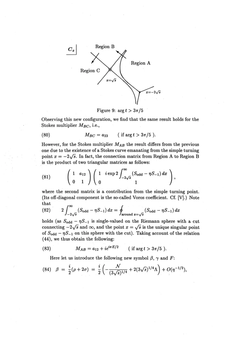
Figure 9: $\arg t>3\pi/5$

Observing this new configuration, we findthat the same result holdsfor the Stokes multiplier $M_{BC}$, i.e.,

(80) $M_{BC}=a_{23}$ (if$\arg t>3\pi/5$ ).

However, for the Stokes multiplier $M_{AB}$ the result differs from the previous

onedue to the existence ofaStokescurveemanating from thesimpleturning

point$x=-2\sqrt{s}$

.

In fact,the connection matrix from Region A toRegion $\mathrm{B}$

is theproduct oftwo triangular matricesas follows:

(81)

$(01$

$i \exp 2\int_{-}\infty 12\sqrt{s}(S1\mathrm{o}\mathrm{d}\mathrm{d}-\eta S-)dx)$ ,

where the second matrix is a contribution from the simple turning point.

(Its off-diagonal component isthe

so-called

Voroscoefficient. Cf. [V].) Note

that

(82) 2$\int_{-2\sqrt{s}}^{\infty}(s_{\mathrm{o}\mathrm{d}\mathrm{d}\eta}-s_{-1})d_{X}=\oint_{\mathrm{a}\Gamma\circ \mathrm{u}\mathrm{n}}\mathrm{d}x=\sqrt{s}(S_{\mathrm{o}\mathrm{d}\mathrm{d}}-\eta S_{-1})d_{X}$

holds (as $s_{\mathrm{o}\mathrm{d}\mathrm{d}}-\eta S-1$ is single-valued on the Riemann sphere with a cut

$\mathrm{c}\mathrm{o}\mathrm{n}\mathrm{n}\mathrm{e}\mathrm{c}\mathrm{t}\mathrm{i}\mathrm{n}\mathrm{g}-2\sqrt{s}$and $\infty$, and the point $x=\sqrt{s}$is the unique singularpoint

of $s_{\mathrm{o}\mathrm{d}\mathrm{d}}-\eta S-1$ on this sphere with the cut). Taking account of the relation

(44), we thus obtain the following:

(83) $M_{AB}=a_{1}2+ie^{i\pi E/2}$ _{(if$\arg t>3\pi/5$ ).}

Here let us introduce the following new symbol $\beta,$

$\gamma$ and $F$:

(85) $\gamma=\frac{i}{2}(\rho-2\sigma)=\frac{i}{2}(-\frac{N}{(3\sqrt{s})^{1/4}}-2(3\sqrt{s})^{1/}4\Lambda \mathrm{I}+O(\eta^{-1/2})$,

(86) $F= \log\{\frac{c_{+}}{C_{-}}e^{i\pi E/4-E/2}(2\sqrt{\eta})\}$

$=- \frac{48\sqrt{3}}{5}s^{5/4}\eta-\frac{E_{0}}{4}\log(263^{5}/2s\eta)5/4+\frac{i\pi E_{0}}{4}+o(\eta^{-1/2})$

.

(We have used (42), (43) and Lemma 1 to obtain the explicit form of the

leading term of each symbol.) Using these symbols, we can summarize the results obtained in this subsection as follows: The Stokes multipliers $M_{AB}$

and $M_{BC}$ (corresponding to the transfer from Region A to Region $\mathrm{B}$ and

from Region$\mathrm{B}$ toRegion $\mathrm{C}$ respectively) of the linear equation (3)$-(30)$ has

the followingexpression:

$(\arg t<3\pi/5)$

(87) $\{$

$M_{AB}$ $=$ $-i\gamma e^{(-F})_{\frac{\sqrt{2\pi}}{\Gamma(E/4+1)}}$

$M_{BC}$ $=$ $\beta e^{(i\pi E/+}\frac{\sqrt{2\pi}}{\Gamma(-E/4+1)}4F)$, $(\arg t>3\pi/5)$

(88) $\{$

$M_{AB}$ $=$ $ie^{i\pi E}-/2i \gamma e^{(}-p)\frac{\sqrt{2\pi}}{\Gamma(E/4+1)}$

$M_{BC}$ $=$ $\beta e^{(i\pi E/+}\frac{\sqrt{2\pi}}{\Gamma(-E/4+1)}4F)$

.

4.4

Connection

formula for $\lambda_{\mathrm{I}}$

.

By the end ofthepreceding sectionwehave succeeded in computing(thefirst few terms of) a pair of Stokes multipliers of the linear equation associated

with the firstPainlev\’e equation. Making useofthis expressionoftheStokes

multipliers, we explicitly determine the connection formula for $\lambda_{\mathrm{I}}$ in the

following way:

Let us consider the followingequation (“$\mathrm{i}_{\mathrm{S}\mathrm{o}\mathrm{m}\mathrm{o}}\mathrm{n}\mathrm{o}\mathrm{d}\mathrm{r}\mathrm{o}\mathrm{m}\mathrm{i}_{\mathrm{C}}$equation”):

(89) $M_{AB}=m_{1}$ and $M_{BC}=m_{2}$,

where $m_{1}$ and $m_{2}$ are given complex constants. Note that $\{M_{AB}, M_{B}c\}$ is

every Stokes multiplier of (3)$-(30)$ can be expressed as a rational function

of $M_{AB}$ and $M_{BC}$ (cf. [K]). Since the Hamiltonian system (2) represents

the condition for isomonodromic deformations of(3)$-(30)$, we can obtain a

solutionof the system (2) (and, hence, of the first Painlev\’eequation (1)) by solving the equation (89) for Aand$N$with regarding$t$and $\eta$ as parameters

for anypair $(m_{1}, m_{2})$ ofcomplex numbers. Keeping this fact in mind, let us

first solve the equation (89) by using the explicit formula (87) of$M_{AB}$ and $M_{BC}$ to obtain a solution of the first Painlev\’e equation when _{$\arg t<3\pi/5$}

.

Then we consider the same equation (89) with the other expression (88)

of $M_{AB}$ and $M_{BC}$

.

Although the expressions of the Stokes multipliers are

different for (87) and (88), the analytic continuation of the solution thus obtained in the region $\{t\in C;\arg t<3\pi/5\}$ should satisfy the _equation

(89) with thesameconstants$m_{1}$ and$m_{2}$ inthe region $\{t\in C;\arg t>3\pi/5\}$

also. Therefore, ifwe solve the equation (89) with the same constants $m_{1}$

and$m_{2}$byusing(88),we canobtainanexplicit representationof the analytic

continuation oftheoriginal solutionin the region $\{\arg t<3\pi/5\}$ to the new

region $\{\arg t>3\pi/5\}$

.

In this way the connection formulaacrossthe Stokes

curve $\{t\in C;\arg t=3\pi/5\}$ should be determined explicitly.

Asanexample, letusinvestigate thecase $m_{1}=m_{2}=0$ in greater detail.

When $\arg t<3\pi/5$, the equation $M_{AB}=M_{BC}=0$ immediately implies

(90) $\beta=\gamma=0$

.

Assuming A and$N$ have the expansion of the form

(91) $\{$

A $=$ $\Lambda_{0}+\eta^{-}\Lambda 1/2+1/2\ldots$

$N$ $=$ _{$N_{0+}\eta^{-1/2}N1/2+\cdots$},

we can easily solve the equation (90). The result is $\Lambda_{0}=N_{0}=0$ (cf. (84)

and (85)$)$ and the corresponding solution of the first Painlev\’e equation (1)

becomes the formal power series solution $\lambda_{\mathrm{I}}$

.

On the other hand, when

$\arg t>3\pi/5$, we still have $\beta=0$ and hence

(92) $E=p^{2}-4\sigma^{2}=-4\beta\gamma=0$

follows from (40), (84) and (85). However, $\gamma=0$ does not hold. Instead we

have to solve the followingsystem of equations: (93) $\beta=0$ and $\sqrt{2\pi}e^{(-F)}\gamma=1$,

or, more explicitly,

(94) $\beta=0$ and $\gamma=\frac{1}{\sqrt{2\pi}}\exp(-\frac{48\sqrt{3}}{5}s^{5/}\eta 4)(1+O(\eta^{-}1/2))$

.

Ifweassumethe expansion(91)again and further regard$\exp(-48\sqrt{3}s^{5/4}\eta/5)$

as aquantity of order$0$in

$\eta$ (justlike in theconstruction of themultiple-scale

solution (10) discussed in [AKT3]$)$, the equation (94) implies

(95) $\Lambda_{0}=i\frac{1}{2\sqrt{\pi}}(12\sqrt{s})-1/4\exp(-\frac{48\sqrt{3}}{5}s^{5/}\eta 4)$ ,

that is,

(96) $\lambda=\sqrt{s}+\eta^{-}i\frac{1}{2\sqrt{\pi}}1/2(12\sqrt{s})-1/4\exp(-\frac{48\sqrt{3}}{5}s\eta 5/4)+\cdots$

.

This expression (96) of$\lambda$ should be the analytic continuation of $\lambda_{\mathrm{I}}$ in the

region $\{\arg t>3\pi/5\}$

.

Thus wehave explicitly determined the connection formula for$\lambda_{\mathrm{I}}$

across

the Stokes

curve

$\{t\in c_{;\arg}t=3\pi/5\}$ as follows:

(97) $\lambda_{\mathrm{I}}$ $arrow$ $\lambda_{\mathrm{I},i/2\sqrt{\pi},0}$

$=$ $\sqrt{s}+\eta-1/2i\frac{1}{2\sqrt{\pi}}(12\sqrt{s})-1/4\mathrm{p}\mathrm{e}\mathrm{x}(-\frac{48\sqrt{3}}{5}s^{s/4}\eta)+\cdots$

.

In particular, by the comparison of (97) and (26) $\sim(28)$ we have

(98) $\mu=\sqrt{\frac{3}{5}}\frac{1}{\pi}=0.24656177\cdots$ ,

which coincides with theprevious numerical result (25) very accurately. This is our determination of the connection formula for $\lambda_{\mathrm{I}}$ by using the

isomonodromic method. In my opinion the isomonodromic method is more

powerful than the argument performed in the previous section (\S 3). (For example, it enables us to determine the undeterminedconstant $\alpha$ (or, more

specifically, $\mu$ in the formula (28)$)$ in a completely explicit manner.) We

hope that this method will determine the connection formula not only for

the formal power series solution $\lambda_{\mathrm{I}}$ but also for any multiple-scalesolution $\lambda_{\mathrm{I},\alpha,\beta}$ with two free parameters. (Here a free parameter means anarbitrary

functionorformalseries of$\eta^{-1/2}$ that is free from$t$

.

See Remark in

\S 2

also.)

However, to realize this expectation we have to compute the connection formula for WKB solutions of the associated linear equation nearthe double turning point $x=\sqrt{s}$, in particular the constants $C_{\pm}$ in (69)$-(70)$, up to

an arbitrarily higher order, and at the $\mathrm{p}\mathrm{r}.\mathrm{e}\mathrm{s}\mathrm{e}\mathrm{n}\mathrm{t}$stage this is still an open

problem.

References

[AKTI] T. Aoki, T. Kawai and Y. Takei: The Bender-Wu analysis and the Voros theory. Special Functions, Springer-Verlag, 1991, pp. 1-29.

[AKT2] –: Algebraic analysis of singular perturbations –on

ex-act WKB analysis –. S\^ugaku, 45 (1993), 299-315. (In Japanese.

English translation is to appear in S\^ugaku Expositions.)

[AKT3] –: WKB analysis of Painlev\’e transcendents with a large

parameter. II. –Multiple-scale analysis ofPainlev\’e

_{transcend.ents.}

Preprint (RIMS-1038).

[BMP] A. Erd\’elyi et al.: Higher Transcendental Functions. Bateman

Manuscript Project (Vol. I, II, III). California Institute of Tech-nology, $\mathrm{M}\mathrm{c}\mathrm{G}\mathrm{r}\mathrm{a}\mathrm{W}$-Hill, 1953.

[DDPI] E. Delabaere, H. Dillinger and F. Pham: R\’esurgence de Voros et

p\’eriodes des courbes hyperelliptiques. Ann. Inst. Fourier (Greno-ble), 43 (1993), 163-199.

[DDP2] –: Exact semi-classical expansions for one dimensional

quantum oscillators. Pr\’epublications _{No. 398, Univ.} Nice-Sophia-Antipolis, 1994.

[FIK] A.S. Fokas, A.R. Its and A.A. Kapaev: On theasymptotic analysis of the Painlev\’e equations via the isomonodromic method.

Nonlin-earity, 7 (1994), 1291-1325. ;

[JK1] N. Joshi and M.D. Kruskal: An asymptotic approach to the

con-nection problem for the first and the second Painlev\’e equations.

Phys. Lett., 130 (1988), 129-137.

[JK2] –: Connection results for the first Painlev\’e equation.

[JMU] M. Jimbo, T. Miwa and K. Ueno: Monodromy preserving defor-mation of linear ordinary differentialequations with rational coef-ficients. I. Physica D, 2 (1981), 306-352.

[K] A.A. Kapaev: Asymptotics of solutions of thePainlev\’e _{equation of}

the first kind. Differential Equations, 24(1989), 1107-1115. $(^{r}\mathrm{b}\mathrm{a}\mathrm{n}\mathrm{S}-$

lated from the Russian original (1988).)

[KT1] T. Kawai and Y. Takei: WKB analysis and deformation of

Schr\"odinger equations. RIMSK\^oky\^uroku,No. 854, 1993, pp. 22-42.

[KT2] –: WKB analysis of Painlev\’e transcendents with a large parameter. I. To appear in Adv. in Math.

[O] K. Okamoto: Isomonodromic deformation and Painlev\’e equations,

and the Garnier systems. J. Fac. Sci. Univ. Tokyo, Sect. IA, 33

(1986), 575-618.

[Tka] K. Takano: His lecture at the workshop and his report in this

vol-ume.

[Tke] Y. Takei: On a WKB-theoretic approach to the Painlev\’e

transcen-dents. To appear in the Conf. Proc. “XIth International Congress of Mathematical Physics (Paris, 1994)”.

[V] A. Voros: The return of the quartic oscillator. The complex WKB