Inflections and singularities on parametric rational cubic curves

Inflections and singularities

on

parametric rational

cubic

curves

鹿大理 酒井 宙 (Manabu Sakai)

$E$ –mail: [email protected]–u.ac.$jp$

1 Introduction

Much attention has been recently been focused on a single- and vector-valued shape

preserving interpolation. There is a considerable literature on numerical methods for

generating shape preserving interpolation; see for example, Sakai

&Usmani

[5], Su

&

Liu [7] and references therein. Parametric cubic curves and useful for generating

vector-valued ”visuallypleasing”, ”shape preserving” interpolantsto a set ofplanar data points.

A drawback of the parametric cubic curves is indicated the fact that unwanted inflection

pointsorsingularity may occur onthese segments. A way of overcoming this problem isto

consider nonlinearapproximation sets, forexample, exponentialsplines, lacunary splines,

rational splines or splines with variable additional nodes. The rational splines have been

of the forms: $\mathrm{q}\mathrm{u}\mathrm{a}\mathrm{d}\mathrm{r}\mathrm{a}\mathrm{t}\mathrm{i}_{\mathrm{C}}/1\mathrm{i}\mathrm{n}\mathrm{e}\mathrm{a}\mathrm{r},$ $\mathrm{c}\mathrm{u}\mathrm{b}\mathrm{i}\mathrm{c}/\mathrm{l}\mathrm{i}\mathrm{n}\mathrm{e}\mathrm{a}\mathrm{r},$ $\mathrm{q}\mathrm{u}\mathrm{a}\mathrm{d}\mathrm{r}\mathrm{a}\mathrm{t}\mathrm{i}_{\mathrm{C}}/\mathrm{q}\mathrm{u}\mathrm{a}\mathrm{d}\mathrm{r}\mathrm{a}\mathrm{t}\mathrm{i}_{\mathrm{C}}$, and $\mathrm{c}\mathrm{u}\mathrm{b}\mathrm{i}\mathrm{c}/\mathrm{q}\mathrm{u}\mathrm{a}\mathrm{d}\mathrm{r}\mathrm{a}\mathrm{t}\mathrm{i}_{\mathrm{C}}$.

For two consecutive data points $z_{i}(=(x_{i}, y_{i})),$ $i=0,1$ and assigned tangent vectors

$z_{i}’(=((x_{i}, y_{i})\prime\prime)$ at these points, we consider a”shape preserving” parametric rational cubic

curve $z(t)=((x(t), y(t)),$$0\leq t\leq 1$, of the form with a parameter $(p\geq 0)$:

(1) $z(t)=Z_{0}(1-t)+z1t+(z’-0z\Delta)\phi(t)+(\Delta_{Z}-z\prime 1)\phi(1-t)$

with $\triangle z=z_{1}-z_{0}$ and $\phi(t)=t(1-t)^{2}/\{1+pt(1-t)\}$. We can easily verify that this form

$z$ satisfies the interpolation relations: $z^{(k)}(0)=z_{0},$$\mathcal{Z}(k)((k)1)=z_{1}^{(k)},$$k=0,1$. A value of

$p=0$willlet $z$ beacubicspline while alarge value of$p$willlet $z$ bean unacceptable”flat”

interpolant. In Section 2, much algebraic manipulation gives the complete distribution

ofinflections and singularity on the curve segment (1). Its use allows us to ensure that

the curve $z$ ofthe form (1) is free from the inflections and singularity (or simply fair) if

$\lambda,$ $\mu\geq 1/(3+p)$ or$\lambda,$$\mu\leq 0$where $\lambda(=(z_{0}’\cross\triangle z)/(z_{0}’\cross z_{1}’))$and$\mu(=-(Z_{1}’\cross\triangle z)/(z’\cross Z’)01)$

the relative lengths of the tangent vectors at the end points with the usual vector product

$’\cross$ ’ where assume that $D(=z_{0}’\cross z_{1}’)\neq 0$, i.e., $z_{i}’,$$i=0,1$ are independent.

Hence, a large value of$p$ can always let the segment $z$ be fair if $\lambda\mu>0$. Another use

ofit also enables us to find another fair curve of the form (1) if $0<\kappa\leq(3+p)\lambda$ and

$0<\eta\leq(3+p)\mu$ where the tangent directions $y_{i}’/x_{i}’,$$i=0,1$ are fixed at the two end

points, and only the magnitudes of the tangents can be varied in scalar multiples $\eta$ and

2 On inflections and singularity

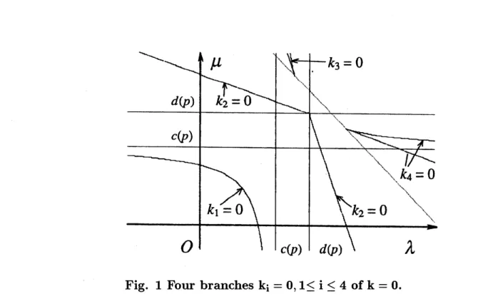
First we note Fig. 1 for $k(\lambda, \mu)=0$ given by the following equation (2):

(2) $k(=k(\lambda, \mu))=4\lambda^{3}\{(3+p)\mu-1\}+4\mu^{3}\{(3+p)\mu-1\}-3\lambda 2\mu 2$

$+\{(3+p)\lambda-1\}2\{(3+p)\mu-1\}2-6\lambda\mu\{(3+p)\lambda-1\}\{(3+p)\mu-1\}=0$.

Fig. 1 Four branches $\mathrm{k}_{\mathrm{i}}=0,1\leq \mathrm{i}\leq 4$ of$\mathrm{k}=0$

.

Inflections. We are now ready to determine the distribution of inflections on the curve

(1). Since $D(=z_{0}’\cross z_{1}’)\neq 0,$ $\Delta_{Z}(=z_{1}-z_{0})$ can be represented as $\Delta z=\mu z_{0}’+\lambda z_{1}’$ where

$(\lambda, \mu)(=C_{0}/D, -C_{1}/D)$ with $C_{i}=z_{i}’\cross\Delta z$.

Defining and doing a fairly lengthy calculation,

(3) $w(t)(=\{\phi’(t)\phi\prime\prime(u)+\phi’’(t)\phi(u)\})=2(1-3tu)(1+ptu)^{3},$$u=1-t$,

inflections of the curve (1) are determined by the equation:

(4) $(z’\cross z^{\prime/})(t)/D(=\lambda\{w(t)-\phi’’(t)\}+\mu\{w(u)-\phi\prime\prime(u)\}-w(t))=0,0<t<1$

or

(5) $\lambda(3u^{2}+pu^{3})+\mu(3t^{2}+pt^{3})+3tu-1=0,0<t<1$.

Letting $t$ be $1/(1+t)$, the above cubic equation (5) can be equivalently rewritten as

We consider several Cases $(\mathrm{a})-(\mathrm{d})$ depending on the values of $\lambda$ and

$\mu$, and for each

case we count the number $N$ of positive roots ofthe cubic equation (6) ( $=\mathrm{t}\mathrm{h}\mathrm{e}$ number

ofinflections on (1) $)$.

(a) $(\lambda-c(p))(\mu-c(p))=0$: In this case, (6) itself or (6) divided by $t$ reduces to a

quadratic equation. Hence, $N=1$ if $\lambda=c(p),$$\mu<c(p)$ or $\lambda<c(p),$$\mu=c(p)$ and $N=0$

if $\lambda=c(p),$$\mu>c(p)$ or $\lambda>c(p),$$\mu=c(p)$.

(b) $\lambda,$$\mu>c(p)$ or $\lambda,$_{$\mu\leq 0$}: In this case, (6) has no positive root. Hence, $N=0$.

For the other cases than $(\mathrm{a})-(\mathrm{b})$, we make a Strum sequence $\{p_{i}(t)\}$ of the cubic

equation (6) for $a^{2}\neq 3b$:

$p_{0}(t)=t^{3}+at^{2}+bt+c(=-p_{0}’(t))=-3t^{2}-2at-b$

(7) $p_{2}(t)=2(a^{2}-3b)t+ab-9c$

$p_{3}(t)=-p_{1}\{(9c-ab)/(2a^{2}-6b)\}(=9k\{4(a^{2}-3b)^{2}\}$

in which

$a=3\lambda/\{(3+p)\lambda-1\},$$b=3\mu/\{(3+p)\lambda-1\},$$C=\{(3+p)\mu-1\}/\{(3+p)\lambda-1\}$

(8)

$k=4a^{3}c+4b^{3}+27c^{2}-18abc-a^{2}b^{2}$_.

Let the integer valued function $s(t)$ bethe number of agreements in sign ofconsecutive

members of the sequence $\{p_{i}(t)\}$

.

Then, the theory of Strum sequences says that the

numbers ofroots in the interval $a<t\leq b$ is given by _$s(b)-S(a)$

.

(c) $(\lambda-c(p))(\mu-c(p))<0$: In this case

assume

_that $\mu<c(p)<\lambda$, the other case $\lambda<c(p)<\mu$ being similarly treated. Then, note that _$a>0$ and _$c<0$

.

When _$b<0$ and

$k>0,$ $\epsilon=\mathrm{S}\mathrm{i}\mathrm{g}\mathrm{n}(ab-9c)<0\Rightarrow s(\mathrm{o})=3$ is contradictory to $s(\mathrm{O})\leq s(+\infty)$, and so $\epsilon>0$.

Table 1 shows that $N(=s(+\infty)-\mathit{8}(\mathrm{o}))=1$.

Table 1. The sequences of signs at $0$ and $\infty$ for $\lambda-c(p))(\mu-c(p))<0$.

$b\backslash k$ positive negative

positive $(-, -, +, +),$ $(+, -, ?,$ $+)$ $(-, -, +, -)(+, -, +*, -)$

negative $(-, +, \epsilon, +),$ $(+, -, +, +)$ $(-, +, ?, -)(+, -, +, -)$

*If$a^{2}-3b<0,$$s(+\infty)=1$ is contradictory to $s(\mathrm{O})(=2)\leq s(+\infty)$, and so $a^{2}-3b>0$.

(d) $0<\lambda,$$\mu<c(p)$: Note that $a<0,$ $b<0$, and $c>0$

.

In addition,

$ab-9c<0$

if

$k>0$as follows. If$ab-9c\geq 0$, i.e., $0<c\leq ab/9$, then we take $k$ as aquadratic equation

in $c$:

Table 2. The sequences of signs at $0$ and $\infty$ for $0<\lambda,$$\mu<c(p)$

.

$k$ positive negative

$(+, +, -, +),$$(+, -, +, +)$ $(+, +, ?, -),$$(+, -, +, -)$

Hence, $N=0$ or 2 for $k\geq 0$ or $k<0$ where the equation $k=0$ in (8) is equivalent

to the equationk $=0$ defined in Lemma 1, strictly speaking, the $k$ in (8) multiplied by

$\{(3+p)\lambda-1\}^{4}/27$ coincides with the $k$ in Lemma 1. For $a^{2}=3b$($\geq\Rightarrow \mathrm{n}\mathrm{o}$ case $(\mathrm{d})$ ), $p_{0}(t)=(t+a/3)^{3}+c-a^{3}/27$ , and so $N=1$ for the case (c). Since for $\lambda,$$\mu<c(p),$ $k=0$

is equal to $k_{1}=0$, we obtain

LEMMA 1 (inflections). If $(\lambda, \mu)\in N_{i},$$0\leq i\leq 2$, the curve (1) has $i$ inflections where

$N_{0}=$

{

$(\lambda,$$\mu)|\lambda,$$\mu\geq c(p)$ or $k_{1}(\lambda,$$\mu)\geq 0$

},

$N_{1}=\{(\lambda, \mu)|(\lambda-c(p))(\mu-c(p))\leq 0$ or

$\lambda=c(p),$$\mu<c(p)$ or $\lambda<c(p),$$\mu=c(p)\}$ and $N_{2}=\{(\lambda, \mu)|k_{1}(\lambda, \mu)<0, \lambda, \mu<c(p)\}$.

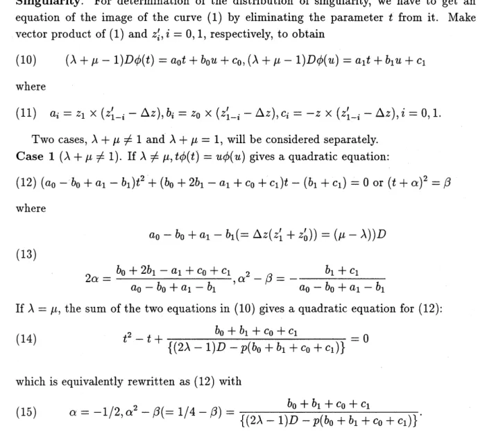
Singularity. For determination of the distribution of singularity, we have to get an

equation of the image of the curve (1) by eliminating the parameter $t$ from it. Make

vector product of (1) and $z_{i}’,$$i=0,1$, respectively, to obtain

(10) $(\lambda+\mu-1)D\phi(t)=a_{0}t+b_{0}u+c_{0},$$(\lambda+\mu-1)D\phi(u)=a_{1}t+b_{1}u+c_{1}$

where

(11) $a_{i}=z_{1}\cross(z_{1-i}’-\Delta z),$ $bi=z0\cross(_{Z_{1i}’}--\triangle z),$$c_{i}=-Z\cross(z_{1-i}’-\Delta z),$$i=0,1$. Two cases, $\lambda+\mu\neq 1$ and $\lambda+\mu=1$, will be considered separately.

Case 1 $(\lambda+\mu\neq 1)$. If $\lambda\neq\mu,$$t\phi(t)=u\phi(u)$ gives a quadratic equation:

(12) $(a_{0}-b_{0}+a_{1}-b_{1})t^{2}+(b_{0}+2b_{1}-a_{1}+c_{0}+c_{1})t-(b_{1}+c_{1})=0$or $(t+\alpha)^{2}=\beta$

where

$a_{0}-b0+a_{1}-b_{1}(=\Delta Z(_{Z_{1}}/+Z_{0})’)=(\mu-\lambda))D$

(13)

$2 \alpha=\frac{b_{0+}2b_{1^{-}}a_{1}+c_{01}+c}{a0-b0+a1-b1},$$\alpha^{2}-\beta=-\frac{b_{1}+c_{1}}{a_{0-}b_{0+a-b}11}$

If $\lambda=\mu$, the sum of the two equations in (10) gives a quadratic equation for (12):

(14) $t^{2}-t+ \frac{b_{0}+b_{1}+C_{0}+C_{1}}{\{(2\lambda-1)D-p(b0+b1+c_{0}+c_{1})\}}=0$ which is equivalently rewritten as (12) with

Hence, let $t^{*}=t+\alpha$ and eliminate the parameter$t^{*}$ (note $(t^{*})^{2}=t+\alpha$ ) from the second

equation in (10) to obtain the equation ofthe image ofthe curve (1):

(16) $\psi(x, y)=(A^{2}\beta-B^{2})=0$

where

(i) $A/D$ $=$ $-(\lambda+\mu-1+p\lambda)(\beta+3\alpha^{2}+2\alpha)+\lambda-(p/D)(2\alpha+1)(b_{1}+c_{1})$

(17)

(ii) $B/D$ $=$ $-(\lambda+\mu-1+p\lambda)(3\alpha\beta+\alpha^{3}+\beta+\alpha^{2})$

$+\alpha\lambda-(1/D)\{p(\alpha^{2}+\beta)+p\alpha-1\}(b_{1}+c1)$.

For$\lambda\neq\mu$, since $\lambda+\mu\neq 1\Leftrightarrow(z_{0^{-}}’\Delta z)\cross(z_{1}’-\Delta z)\neq 0,$$(Z_{1-i^{-}}\Delta z)\cross z=c_{i},$$i=0,1$in (11)

enable us to consider $(x, y)$ as functions of $(C_{0}, c_{1})$, and in addition the second and third

equationsin (13) (i.e., $2\alpha(\mu-\lambda)D=b_{0+}2b_{1}-a_{1}+c_{0}+C_{1}$ and $b_{1}+c_{1}=-(\mu-\lambda)(\alpha 2-\beta)D$)

$)$ enable $(C_{0}, c_{1})$ as $(\alpha,\beta)$. Then, the singularity of$\psi=0$ of$(\alpha,\beta)$ for $(x, y)$ is determined

by the system ofequations

(18) $\psi(\alpha, \beta)=\psi\alpha(\alpha,\beta)=\psi_{\beta}(\alpha,\beta)=0$

i.e.,

(19) $A^{2}\beta=B^{2},2AA_{\alpha}\beta=2BB_{\alpha},$_{$2AA_{\beta}\beta+A^{2}=2BB_{\beta}$}

.

where by (13), $(b_{1}+c_{1})/D=-(\mu-\lambda)(\alpha 2-\beta)$ and so (17) reduce to

(i) $A/D$ $=$ $-(\lambda+\mu-1+p\lambda)(\beta+3\alpha^{2}+2\alpha)+\lambda+p(2\alpha+1)(\mu-\lambda)(\alpha^{2}-\beta)$

(20)

(ii) $B/D$ $=$ $-(\lambda+\mu-1+p\lambda)(3\alpha\beta+\alpha^{3}+\beta+\alpha^{2})$

$+\alpha\lambda+(\mu-\lambda)(\alpha 2-\beta)\{p(\alpha^{2}+\beta)+p\alpha-1\}$.

For $\lambda=\mu$, we consider $\psi(=A^{2}\beta-B^{2})$ as function of $(c0, c_{1})$ with $A,$ $B$ and $\beta$ defined

by (15) and (17). Then, the singuraity is determined by the system ofequations:

(21) $\psi(c_{0}, c_{1})=\psi_{C}0(_{C}0, c_{1})=\psi \mathrm{C}_{1}(c_{0,1}C)=0$

.

Here note that if there were any singularity (loop or cusp) on the curve segment (1),

two values of the parameter$t$ defined by the quadratic equation $(t+\alpha)^{2}=\beta$ must belong

to $(0,1)$, i.e.

where $\beta>0$ and $\beta=0$ correspond to aloop and cusp, respectively For (18) (i.e., (19))

and (21), two cases $A\neq 0$ and $A=0$, will be considered separately.

(a) $A\neq 0$: First we note $\beta\neq 0$ from (19). If$\lambda\neq\mu$ , from (19) we obtain the following

relations according to the sign of $B/A$:

(i) $B=A\sqrt{\beta},$$B_{\alpha}=A\sqrt{\beta}\alpha’=A2\sqrt{\beta}(B\beta-\sqrt{\beta}A\beta),$$B=2\beta(B\beta-\sqrt{\beta}A\beta)$

(23)

(ii) $B=-A\sqrt{\beta},$$B_{\alpha}=-A\sqrt{\beta}\alpha’ A=-2\sqrt{\beta}(B\beta+\sqrt{\beta}A_{\beta}),$ $B=-2\beta(B\beta+\sqrt{\beta}A_{\beta})$

For $23(\mathrm{i})(\Leftrightarrow B/A>0)$, by (20) $B_{\alpha}=A_{\alpha}\sqrt{\beta}$ reduces to

(24) $-(\lambda+\mu-1+p\lambda)(3\beta+3\alpha^{2}+2\alpha)+\lambda$ $+(\mu-\lambda)\{p(2\alpha+1)(\alpha^{2}-\beta)+2p\alpha(\beta+\alpha 2)+2\alpha(p\alpha-1)\}$ $=$ $\sqrt{\beta}\{-(\lambda+\mu-1+p\lambda)(6\alpha+2)+p(\mu-\lambda)(6\alpha^{2}-2\beta+2\alpha)\}$ From $A=2\sqrt{\beta}(B_{\beta}-\sqrt{\beta}A_{\beta})$

,

by (20) (25) $-(\lambda+\mu-1+p\lambda)(3\beta+3\alpha+22\alpha)+\lambda+p(\mu-\lambda)(2\alpha^{3}-2\alpha\beta+\alpha^{2}-\beta)$ $=2\sqrt{\beta}\{-(\lambda+\mu-1+p\lambda)(3\alpha+1)+p(\mu-\lambda)(\alpha-2\beta)-p(\alpha+\beta 2)-p\alpha+1\}$ $-2\beta\{p(\mu-\lambda)(-2\alpha-1)\}$.

On subtracting from (24) to (25), we obtain a cubic equation in $\sqrt{\beta}(=u)$:

(26) $(u-\alpha)\mathrm{t}p(u-\alpha)2-p(u-\alpha)-1\}=0$

where for $23(\mathrm{i}\mathrm{i})(\Leftrightarrow B/A<0)$, we have only to change the coefficient of $\sqrt{\beta}$ in (26).

These cubic equations in $\sqrt{\beta}$ have no roots satisfying the required inequalities in (22),

i.e., $\beta<\alpha^{2}(-1/2\leq\alpha<0)$ or $\beta<(1+\alpha)^{2}(-1<\alpha<-1/2)$ where for $p=0,$ (26)

reduces alinear equation having no root satisfying (22). When $\lambda=\mu,$ (21) give

(27) $2AA_{c:}\beta+A^{2}\beta C_{\iota}=2BB_{c_{t}},$$i=0,1$

where by (17), $A_{c_{1}}-A_{c0}=-p(2\alpha+1),\beta_{c_{1}}-\beta_{c_{0}}=0,$$B_{c_{1}}-B_{c_{0}}=-p(\alpha+\beta 2+\alpha)+1$

Note that $\beta\neq 0$. If$\beta=0,$$A=0$ would come from (27) since $\beta=0$ gives $B=0$ and $\beta_{c_{1}}(=\beta_{c_{0}})=\{(2\lambda-1)D\}/\{(2\lambda-1)D-p(b_{0}+b_{1}+c_{0}+c_{1})\}^{2}\neq 0$ where $\lambda=\mu$ and

$\lambda+\mu\neq 1$. A difference oftwo equations (27) gives$p(2\alpha+1)A\beta=B\{p(\alpha^{2}+\beta)+p\alpha-1\}$.

Since $B=A\sqrt{\beta}$ for $A\neq 0$, we obtain the quadraic equation in $u(=\sqrt{\beta})$ being equal to

the quadratic factor in the braces in (26) where for $B=-A\sqrt{\beta}$, the coefficient of $\sqrt{\beta}$ is

to be changed. That is, in the case $A\neq 0$, the curve (16) does not have a singularity.

(22), while determining the singularity, we can assume that $\alpha^{2}-\beta\neq 0$ and $\alpha\neq 0$. On

making $20(\mathrm{i})\cross(\beta+\alpha^{2})-20(\mathrm{i}\mathrm{i})\cross(2\alpha)$,

(28) $\alpha^{2}-\beta=-\frac{\lambda+2\alpha(\lambda-\mu)}{\lambda+(1+p)\mu-1}(\neq 0)$

Substitute (28) into $17(\mathrm{i})$ for $\alpha^{2}-\beta$ to obtain

(29) $2 \alpha=\frac{(\lambda+\mu-1)(1-2\lambda)-p(4\lambda\mu-\lambda-\mu)-p^{2}\lambda\mu}{(\lambda+\mu-1)^{2}+p(4\lambda\mu-\lambda-\mu)+p^{2}\lambda\mu}(\neq 0)$

where the denominator of (29) is positive for $(\lambda, \mu)\neq(d(p), d(p))$. Eliminate $\alpha$ from

(28)$-(29)$ to obtain

(30) $4 \beta=\frac{4\kappa(\lambda,\mu)}{\{(\lambda+\mu-1)^{2}+p(4\lambda\mu-\lambda-\mu)+p^{2}\lambda\mu\}2}$

In addition, from (28)$-(29)$, note

(i) $\alpha^{2}-\beta=\frac{\lambda^{2}+\mu-\lambda\mu(3+p)}{(\lambda+\mu-1)^{2}+p(4\lambda\mu-\lambda-\mu)+p^{2}\lambda\mu}$

(31)

(ii) $(1+ \alpha)^{2}-\beta=\frac{\mu^{2}+\lambda-\lambda\mu(3+p)}{(\lambda+\mu-1)^{2}+p(4\lambda\mu-\lambda-\mu)+p^{2}\lambda\mu}$.

Herewe consider the case $\alpha\in(-1/2,0)$, the othercase $\alpha\in(-1, -1/2)$ similarly treated.

Then, (30)$-(31)$ imply that the singularity

occurs

if$\kappa(\lambda, \mu)\geq 0$ and in addition if

(i) $(\lambda+\mu-1)(\mu-\lambda)>0(\Leftrightarrow-1/2<\alpha)$

(32) (ii) $\mu\{(2+4p+p^{2})\lambda-(1+p)\}>-2\lambda^{2}+(3+p)\lambda-1(\Leftrightarrow\alpha<0)$

(iii) $\lambda^{2}>\{(3+p)\lambda-1\}\mu(\Leftrightarrow\alpha^{2}>\beta)$

.

Next we consider the case $\lambda=\mu$, i.e.,$\alpha=-1/2$. Then, from $17(\mathrm{i}),$ $1/4-\beta=$

$-\lambda/\{(2+p)\lambda-1\}$ from which (i) $\beta=0(\Rightarrow \mathrm{a}\mathrm{c}\mathrm{u}\mathrm{s}\mathrm{P})\Leftrightarrow\lambda=1/(6+p)$ and (ii) $0<\beta<1/4$

$(\Rightarrow \mathrm{a}\mathrm{l}\mathrm{o}\mathrm{o}_{\mathrm{P}})\Leftrightarrow 0<\lambda<1/(6+p)$. Note that $(\lambda, \mu)=(1/(6+p), 1/(6+p))$ is on the first

branch $k_{1}=0$.

Case 2 $(\lambda+\mu=1)$ In this case, it is easy to show that neither inflection nor singularity

occurs.

Summarizing the above two cases, $\lambda+\mu\neq 1$ and _{$\lambda+\mu=1$}, we obtain a lemma

concerning the distribution of the singularity on the curve (1).

LEMMA 2 (singularity). If$(\lambda, \mu)\in L$ or $C,\mathrm{t}\mathrm{h}\mathrm{e}\mathrm{n}$a loop or cusp occurs on the curve (1)

$C=\{(\lambda, \mu)|k_{1}(\lambda, \mu)=0\}$.

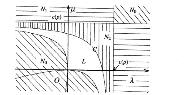
THEOREM. (Inflections and singularity). Assume that $\Delta z=\mu z_{0}’+\lambda z_{1}’$. Then,

Fig-ure 2 gives the distribution of inflections and singularity on the curve of the form (1)

with respect to $(\lambda, \mu)$ where $N_{i},$$0\leq i\leq 2$ represent the regions for which the curve has

$i$-inflections and no singularity.

REMARK. A larger value of$p$ for shape control might bring a larger interpolation

er-ror and the resulting curve would be an unacceptable ”flat” interpolant while a choice

of$p=0$ yields a fourth order interpolation ([9]). Therefore, Theorem 1 suggests us to

take $p=0$ for $\rho(=\min(\lambda, \mu))\geq 1/3$ and $p=1/\rho-3$ for _$0<\rho<1/3$, respectively.

The following technique for eliminating the unwanted inflections and singularity on

the curve (1) (as is usual with the case $p=0$ ) has been also used ([7]). Suppose that

the tangent directions are fixed at the two end points, and only the magnitudes of the

tangents are allowed to be varied in scalar multiples $\eta$ and $\kappa(\eta, \kappa>0)$, respectively.

Since $C_{0}arrow\eta C_{0},$$C_{1}arrow\kappa C_{1},$$Darrow\eta\kappa D$, Theorem gives the following corollary concerning

the existence of the region $(\eta, \kappa)$ for which the corresponding curve (1) is fair.

COROLLARY (Theorem [7, p. 54]). Assume that $\lambda$ and

$\mu>0$. Then the curve of

the form (1) is fair for $0<\kappa\leq(3+p)\lambda$ and $0<\eta\leq(3+p)\mu$.

Fig. 2. Distribution of inflections and singularity.

Finally weconsider the different shapesof the curves with different values of$p$; see Fig.

$0,1$. Since $(\lambda, \mu)=(2/17,1/17),p=4.21$ and $p=14$ are an approximate value when a

cusp occurs and the proposed value in Remark, respectively.

Fig. 3. Different shapes of$\mathrm{c}\mathrm{u}\mathrm{r}\mathrm{v}\mathrm{e}$

(

segments with different values $p$

.

References

1. Delbourgo,R., Gregory, J.$\mathrm{A}.(1985)$: Shapepreserving piecewise rational interpolation.

SIAM J. Sci. Statist. Comput. 6, 967-976.

2. Sakai, M., Lop\’ez de Silanes, M. C. (1986): A simple rational splines and its application

to monotonic interpolation to monotonic data. Numer. Math. 50, 171-182.

3. Sakai, M., Schmidt, J. W. (1989), Positive interpolation with rational splines. BIT 29,

140-147.

4. Sakai, M., Usmani, R. (1990): On orders of approximation of plane curves by rational

splines. BIT 30,

735-741.

5. Sakai, M., Usmani, R.: On fair parametric rationalcurves (to appear in BIT).

6. Sp\"ath, H. (1990): Eindimensionale $\mathrm{S}\mathrm{p}\mathrm{l}\mathrm{i}\mathrm{n}\mathrm{e}-\mathrm{I}\mathrm{n}\mathrm{t}\mathrm{e}\mathrm{r}\mathrm{p}_{0}1\mathrm{a}\mathrm{t}\mathrm{i}\mathrm{o}\mathrm{n}\mathrm{S}- \mathrm{A}\mathrm{l}\mathrm{g}\mathrm{o}\mathrm{r}\mathrm{i}\mathrm{t}\mathrm{h}\mathrm{m}\mathrm{e}\mathrm{n}$. R. Oldenbourg

Verlag, Munchen.

7. Su, B-Q., Liu, D-Y. (1989): Computational Geometry-Curve and Surface Modeling.