Pattern formation in a two-layered Benard convection (Mathematical Analysis in Fluid and Gas Dynamics)

Pattern formation in

atw0-layered

B\’enard

convection

鳥取大・工 藤村 薫 (Kaoru Fujimura)

Department

_of

Applied Mathematics and Physics

Tottori University, Tottori 680-8552, Japan

The resonant interaction between steady modes with wavenumbers in the ratio 2:1 has been examined

for its pattern formation on a hexagonal lattice. Twelvedimensional amplitude equations of the cubic

order arederived by meansof thecenter manifold reduction. With theaid of theequivariant bifurcation

theory, steady solutions of the equations duetothe primary and the secondarybifurcations areclassified

and the orbital stability of them are analyzed. The analyses are extended to twolayered

Rayleigh-B\’enardconvectionwithanon-deformablethin interface, which providestheexact resonancebetween the

critical modesas had been found by Proctor and Jones [10]. In order for the cubic amplitude equations

to be generic, the self-adjointness of the operators in the linearized problem needs to be broken. For

this purpose, we took account of the quadratic density profile as afunction of the temperature. All

the primary and the secondary steady patterns obtained are found tobe unstable except for the super

hexagonal patternwhichis composed of hexagonal pattern and double sized one.

1. Introduction

In the presence of $\mathrm{O}(2)$-symmetry, the resonant interaction between steady modes with

wavenumbers in the ratio 2:1 is governed by

$\dot{z}_{1}=f_{1}(z_{1}, z_{2}, \mu)$, $\dot{z}_{2}=f_{2}(z_{1}, z_{2}, \mu)$, $z_{1}$,$z_{2}\in \mathrm{C}$, $\mu\in \mathrm{R}^{2}$, (1)

where the vectorfield is expressed in terms of$\mathrm{O}(2)$-equivariant polynomials and invariant

func-tions

auch

that

$f_{1}(z_{1}, z_{2}, \mu)=z_{1}p_{1}(u, v, w, \mu)+\overline{z}_{1}z_{2}q_{1}(u, v, w, \mu)$,

$f_{2}(z_{1}, z_{2}, \mu)=z_{2}p_{2}(u, v, w, \mu)+z_{1}^{2}q_{2}(u, v, w, \mu)$

.

(2) Here, $u=|z_{1}|^{2}$, $v=|z_{2}|^{2}$, and $w=\overline{z}_{1}^{2}z_{2}+z_{1}^{2}\overline{z}_{2}$

are

$\mathrm{O}(2)$-invariants, $z_{1}$, $z_{2},\overline{z}_{1}z_{2}$, and $z_{1}^{2}$

are

generators of the $\mathrm{O}(2)$-equivariant vector field, and$\mathrm{p}\mathrm{i}$,

$p_{2}$, $q_{1}$, and $q2$

are

real valued invariant

functionsof$u$, $v$, and $w$

.

See Buzano and Russo [3] for further details.

TaylorexpandingPi, $p_{2}$, $q_{1}$, and $q_{2}$ about the origin and truncating the resultant equations

at the cubic order

we

obtain

$\dot{z}_{1}=\sigma_{1}z_{1}+\beta_{1}\overline{z}_{1}z_{2}+\lambda_{11}|z_{1}|^{2}z_{1}+\lambda_{21}|z_{2}|^{2}z_{1}$,

$\dot{z}_{2}=\sigma_{2}z_{2}+\beta_{2}z_{1}^{2}+\lambda_{12}|z_{1}|^{2}z_{2}+\lambda_{22}|z_{2}|^{2}z_{2}$

.

(3)

Analyses

on

the steadystatesolutionsof (3) have beendone,$\mathrm{e}\mathrm{g}.$,by Dangelmayr[5], in detail.

Equations (3) have threenon-trivialsteadystatesolutions

as

fixedpoints. They

are

steadystate

$\mathrm{S}_{2}$ given by $u=0$ and $v=0$, and asymmetric steady states $\mathrm{S}\pm \mathrm{g}\mathrm{i}\mathrm{v}\mathrm{e}\mathrm{n}$ by $u$,$v>0$, $z_{2}\in \mathrm{R}$, and

$\cos[2\arg(z_{1})-\arg(z_{2})]=\pm 1$

.

As relative equilibria, atraveling

wave

bifurcates from $\mathrm{S}\pm\cdot$ It

has the property that $u$,$v>0$, $\frac{d}{dt}[2\arg(z_{1})-\arg(z_{2})]=0$, and $\cos[2\arg(z_{1})-\arg(z_{2})]=\pm 1$

.

Standingwavesbifurcate from the asymmetric steady states whereas modulated

waves

bifurcate

from the traveling

wave

due to Hopf bifurcation. Proctor and Jones [10] and Armbruster

数理解析研究所講究録 1247 巻 2002 年 79-96

Guckenheimer and Holmes [1] clarified the existence of structurally stable heteroclinic cycles.

Very recently,

new

heteroclinic cycles far from the mode interaction point were extensively

investigated by Porter and Knobloch[9]. So far, all the results above exhibit

one

dimensional

variation in the planform: the spatial pattern caused by the resonance varies periodically in

one

horizontal direction. Aquestion naturaly arises whether the solutions mentioned above

are

stable in theframeworkoftw0- imensional patternformationproblem. Standard wayto

answer

the question is to examine the

resonance

on

asquare

or

ahexagonal lattice. We focus ourselves

on

the pattern formation

on

the latter lattice.

2. Eigenfunction expansion and center manifold reduction

In this section,

we

formally derive the amplitude equations governing the weakly nonlinear

evolution of exactly resonating modes

on

ahexagonal lattice.

We assume our

physical system

has

an

infinite extent inthe horizontal $xy$-plane. Consider asituation where threedimensional

disturbance $\psi(x,y, z,t)$ is added to the basic field which is homogeneous and isotropic in the

horizontal plane. Here, the vector $\psi$ may be composed of velocity, temperature, magnetic field,

etc. Let

us

start with the nonlinear PDE governing $\psi(x, y, z,t)$ having the form

$\frac{\partial}{\partial t}S\psi$ _{$=\mathcal{L}(\mu)\psi+N(\psi,\psi)$}, (4)

where $S$ and $\mathcal{L}$ denote linear operators involvingspatial derivatives, $N$denotesquadratic

non-linear terms, and $\mu\in \mathrm{R}^{2}$ denote control parameters. These$S$, $\mathcal{L}$, and$N$

are

assumed to have

no

explicit dependence

on

either$x$, $y$,

or

$t$

.

Explicit form of$S$,$\mathcal{L}$, and$N$$\mathrm{w}\mathrm{i}\mathrm{U}$ be given in

\S 4

for

tw0-layered Rayleigh-B\’enard convection.

2.1. Expansions inFourier series and linear eigenfunctions

The linearizedequations of (4) subject to appropriate boundary conditionsprovide alinear

eigenvalue problem. We

assume

the eigenvalues discrete andsimple. Denote the$j$-th eigenvalue

by$\sigma^{(j)}$ and the eigenfunction belonging to $\sigma^{(j)}$ by $\psi^{(\mathrm{j})}$

.

The eigenvalue problem is given by $\mathcal{L}(\mu)\psi^{[\mathrm{j})}(x,y, z)=\sigma^{(j)}S\psi^{(j)}’(x,y,$z), j $\geq 1$, (5)

with appropriate boundary conditionsfor$\psi^{(j)}$

.

Let the eigenvalues$\sigma^{(j)}$ b

$\mathrm{e}$ordered in

adescend-ing manner such that

${\rm Re}\sigma^{(1)}>{\rm Re}\sigma^{(2)}>{\rm Re}\sigma^{(3)}>\cdots$

.

We

assume

that $\mathrm{R}\epsilon$ $\sigma^{(1)}=0$ and ${\rm Re}\sigma^{(j)}<0$ for

$j\geq 2$

.

The corresponding eigenfunction

$\psi^{(1)}(x, y, z)$ belonging to$\sigma^{(1)}$ is assumed to be alinear combination of twelve

exponentialfactors

$\mathrm{e}^{\pm_{\dot{l}}k_{c}x}$, $\mathrm{e}^{\mathrm{f}\mathrm{i}k_{\mathrm{c}}(\frac{-1}{2}x+_{2}^{\mathrm{L}3}y}.)$, $\mathrm{e}^{\pm:k_{\mathrm{c}}\mathrm{t}-\frac{1}{2}x-L_{2}^{\mathrm{s}_{y)}}}$

,

$\mathrm{e}^{\pm 2:k_{\mathrm{c}}x}$, $\mathrm{e}^{\pm 2\dot{l}k_{\mathrm{c}}(\frac{-1}{2}x+^{L_{2}3}y})$, $\mathrm{e}^{\pm 2:k_{\mathrm{c}}\mathrm{t}^{-\frac{1}{2}x-\mathrm{L}_{2}3}u)}$

.

(6)

We set

$E_{1}=\mathrm{e}^{k_{\mathrm{c}}x}.\cdot$, $E_{2}=\mathrm{e}^{:k_{\mathrm{c}}(\frac{-1}{2}x+\frac{\sqrt{3}}{2}y})$

.

(7)

All the factors

in

(6)

are

expressed in terms of$E_{1}$ and

a

as $E_{1}^{m}E_{2}^{n}$ for m,n $\in \mathrm{Z}$

.

Especially

$\mathrm{e}^{\pm_{\grave{l}}k_{\mathrm{C}}\mathrm{t}-\frac{1}{2}x-L_{2}\epsilon_{y)}}=E_{1}^{\mp 1}E_{2}^{\mp 1}$

.

We Fourier decompose $\psi^{(j)}(x, y, z)$ as

$\psi^{(j)}=\sum_{m,n}\phi_{mn}^{(j)}(z)E_{1}^{m}E_{2}^{n}$. (8)

The Fourier coefficient $\phi_{mn}^{(j)}(z)$ satisfies the linear eigenvalue

problem

$L_{mn}(\mu)\phi_{mn}^{(j)}=\sigma_{mn}^{(j)}S_{mn}\phi_{mn}^{(j)}$, (9)

subject to appropriate boundary conditions for $\phi_{mn}^{(j)}$

where

$L_{mn}=\mathcal{L}|_{\partial_{x}arrow i(m-\frac{n}{2})nk_{\mathrm{c}},\partial_{z}arrow d/dz}k_{\mathrm{c}},\partial_{\nu^{arrow i}}\mathrm{L}_{2}3$,

$S_{mr1}=S|_{\partial_{x}arrow i(m-\frac{n}{2})k_{c},\partial_{y}arrow i\frac{\sqrt{3}}{2}nk_{\mathrm{c}},\partial_{z}arrow d/dz}$

.

The adjoint problem corresponding to (9) is defined by

$\overline{L}_{mn}(\mu)\overline{\phi}_{mn}^{(j)}=\sigma_{mn}^{(j)}\tilde{S}_{mn}\tilde{\phi}_{mn}^{(j)}$, (10)

with

$\langle\tilde{\phi}_{mn}^{(j)}, (L_{mn}(\mu)-\sigma_{mn}^{(j)}S_{mn})\phi_{mn}^{(j)}\rangle=\langle(\tilde{L}_{mn}(\mu)-\sigma_{mn}^{(j)}\tilde{S}_{mn})\tilde{\phi}_{mn}^{(j)}, \phi_{mn}^{(j)}\rangle$ ,

where $\langle$ ,$\rangle$ denotes

an

appropriate inner product.

We

assume

that all the linear eigenvalues $\sigma_{mn}^{(j)}$

axe

simple and the eigenfunctions $\phi_{mn}^{(j)}$

be-longing to $\sigma_{mn}^{(j)}$

are

orthogonal and complete. Let us now expand $\psi(x, y, z, t)$ in Fourier series

and linear eigenfunctions:

$\psi(x, y, z,t)$ $= \sum_{m=-\infty}^{\infty}\sum_{n=-\infty}^{\infty}\sum_{j=1}^{\infty}\vee A_{mn}^{(j)}(t)\phi_{mn}^{(j)}(z)E_{1}^{m}E_{2}^{n}$

.

(11)

The reality condition gives$A_{-marrow n}^{(j)}=\overline{A}_{mn}^{(j)}$ where

an

overbar denotes the complex conjugate.

Substituting (11) into (4) and taking the inner products with the adjoint functions $\tilde{\phi}_{mn}^{(j)}$, we

obtain amplitude equations for$A_{mn}^{(j)}$:

$\dot{A}_{mn}^{(j)}=\sigma_{mn}^{(\dot{j})}(\mu)A_{mn}^{(j)}+\sum_{k,l}\lambda_{k,l,m-k,n-l}^{(j,p,q)}A_{k,l}^{(p)}A_{m-k,n-l}^{(q)}$, (12)

where

$\sigma_{mn}^{(j)}(\mu)=\frac{\langle\tilde{\phi}_{mn}^{(j)},L_{mn}(\mu)\phi_{mn}^{(j)}\rangle}{\langle\tilde{\phi}_{mn}^{(j)},S_{mn}\phi_{mn}^{(j)}\rangle}$ , $\lambda_{k,i,m-k,n-l}^{(jp,q)}=\frac{\langle\tilde{\phi}_{mn}^{(j)},N(\phi_{kl}^{(p)},\phi_{m-k,n-l}^{(q)})\rangle}{\langle\tilde{\phi}_{mn}^{(j)},S_{mn}\phi_{mn}^{(j)}\rangle}$

.

2.2. Center manifold reduction

The center manifold theorem guarantees that the amplitude of stable modes $A_{mn}^{(j)}$

with

$(m, n,j)=(\pm 1,0,1)$_, $(0, \pm 1,1)$, $(\mp 1, \mp 1,1)$, $(\pm 2,0,1)$, $(0, \pm 2,1)$, $(\mp 2, \mp 2,1)$ is expressed by

$A_{mn}^{(j)}=h_{mn}^{(j)}(A_{\pm 10}^{(1)}, A_{0\pm 1}^{(1)}, A_{\mp 1\mp 1}^{(1)}, A_{\pm 20}^{(1)}, A_{0\pm 2}^{(1)},A_{\mp 2\mp 2}^{(1)})$

.

(8)

See

[4]. Thefunction $h_{mn}^{(j\rangle}$

satisfies$h_{mn}^{(j)}(0)=dh_{mn}^{(j)}(0)=0$_where $dh_{mn}^{(j)}$ is the Jacobianderivative

of$h_{mn}^{(j)}$

.

We mayexpand$h_{mn}^{(j)}$ in$\mathrm{t}\mathrm{e}$ rmsof$A_{\pm 10}^{(1)}$,$A_{0\pm 1}^{(1)}$,$A_{\mp 1\mp 1}^{(1)}$,$A_{\pm 20}^{(1)}$,$A_{0\pm 2}^{(1)}$, and$A_{\mp 2\mp 2}^{(1)}$andtruncat$\mathrm{e}$

(13) at the quadratic order in order to derive the cubic amplitude equations. Therefore $h_{mn}^{(j)}$ i $\mathrm{s}$

expressed

ae

$h_{mn}^{(j)}= \sum_{k_{1},k_{2\prime}l_{1\prime}l_{2}}\gamma_{k_{1}k_{2}l_{1}l_{2}}^{(j)}A_{k_{1}k_{2}}^{(1)}A_{l_{1}l_{2}}^{(1)}+O(3)$

.

(14)

Substituting (14) into (12) for the amplitudes spanningthe stable manifold,

we

have

$\gamma_{k_{1}k_{2}l_{1}l_{2}}^{(j)}=\frac{\lambda_{k_{1}k_{2}l_{1}l_{2}}^{(j11)}}{\sigma_{k_{1}k_{2}}^{(1)}+\sigma_{l_{1}l_{2}}^{(1)}-\sigma_{k_{1}+k_{2\prime}l_{1}+l_{2}}^{[\mathrm{j})}}$

.

(15)

Substitution

of(15)into (12)for$A_{\pm 1,0}^{(1)}$, $A_{0,\pm 1}^{(1)}$,$A_{\pm 1,\pm 1}^{(1)}$,$A_{\pm 2,0}^{(1)}$,$A_{0\pm 2}^{(1)}$,

a

$\mathrm{d}$$A_{\pm 2,\pm 2}^{(1)}$yields

twelve-dimensional amplitude equations for themselves. We

now

simplify the notations by changing

$A_{10}^{(1)}arrow z_{1}$, $A_{01}^{(1)}arrow z_{2}$, $A_{-1-1}^{(1)}arrow z_{3}$, $A_{20}^{(1)}arrow z_{4}$, $A_{02}^{(1)}arrow z_{5}$, and $A_{-2-2}^{(1)}arrow z_{6}$

.

The amplitude

equations truncated at the cubic order

are

obtained

as

$\dot{z}_{1}=\sigma_{1}z_{1}+\delta_{1}\overline{z}_{2}\overline{z}_{3}+\beta_{1}\overline{z}_{1}z_{4}+[\kappa_{11}|z_{1}|^{2}+\kappa_{12}(|z_{2}|^{2}+|z_{3}|^{2})]z_{1}$

$+[\mu_{11}|z_{4}|^{2}+\mu_{1}2(|z_{5}|^{2}+|z_{6}|^{2})]z_{1}+\nu_{1}\overline{z}_{1}\overline{z}_{5}\overline{*}+\xi_{1}z_{2}z_{3}z_{4}+\eta_{1}(\overline{z}_{2}z_{3}\overline{*}+z_{2}\overline{z}_{3}\overline{z}_{5})$,

$\dot{z}_{4}=\sigma_{2}z_{4}+\delta_{2}\overline{z}_{5}\overline{z}\epsilon+\beta_{2}z_{1}^{2}+[\kappa_{21}|z_{1}|^{2}+\kappa_{22}(|z_{2}|^{2}+|z_{3}|^{2})]z_{4}$

$+[\mu_{21}|z_{4}|^{2}+\mu_{22}(|z_{5}|^{2}+|z_{6}|^{2})]z_{4}+\iota az_{1}\overline{z}_{2}\overline{z}_{3}+\xi_{2}(\overline{z}_{3}^{2}\overline{z}_{5}+\overline{z}_{2}^{2}\overline{z}_{6})$, (16)

We set $\sigma_{1}=\sigma_{10}^{(1)}$ and $\sigma_{2}=\sigma_{20}^{(10)}$

.

The

1near

terms $\sigma_{1}z_{1}=\sigma_{10}^{(1)}z_{1}$ and$\sigma_{2}z_{4}=\sigma_{20}^{(1)}z_{4}$

are

retained

in (16) although

we

have already assumed that$\sigma_{10}^{(1)}=\sigma_{20}^{(1)}=0$ at the verybeginingof the above

formal analysis. We $\mathrm{w}\mathrm{i}\mathrm{U}$ change

$\sigma_{1}$ and $\sigma_{2}$

as

bifurcation parameters, later. The remaining

equationsfor$z_{2}$, $z_{3}$, $z_{5}$, and $z_{6}$

are

readilyobtainedbycyclic changesofthe subscripts attached

to $z$

.

3. Steady solutions and their orbital stability

In this section, we

assume

that the centre manifold reduction has already been carried out

not only up tothe cubicorder, but up to

an

arbitraryorderofapproximation. We firstgivethe

generalform of the amplitude equations in thepresence ofthe hexagonal lattice symmetry. We

then analyze the steady solutionsofthe amplitude equations and theirorbitalstabilitywith the

aidofthe equivariant bifurcation theory. The results of this section

are

useful when

we

analyze

the steady solutions and theirorbital stability for (16), systematically.

The amplitude equations $\dot{z}=g(z, \lambda)$, $g:\mathrm{C}^{6}\mathrm{x}\mathrm{R}^{2}arrow \mathrm{C}^{6}$ for

z$=(\mathrm{z}\mathrm{i}\{\mathrm{i}),$$z_{2}(t),z_{3}(t),z_{4}(t)$,$z_{5}(t)$,$z_{6}(t))\in \mathrm{C}^{6}$, $\lambda\in \mathrm{R}^{2}$ (17)

are

generated bythe vector fields

$g(z, \lambda)=(g_{1}(z, \lambda),g_{2}(z, \lambda),g_{3}(z, \lambda),g_{4}(z, \lambda),g_{5}(z, \lambda),g\epsilon(z, \lambda))$

.

(18)

In the presence of asymmetry group $\Gamma$, the vector field $g(z, \lambda)$ is said to be equivariant

under

an

action of$\Gamma$ if

$g(\gamma z)=\gamma g(z)$ for

au

$\gamma\in\Gamma$ (19)

holds. For the hexagonal lattice symmetry, $\Gamma=D_{6}\dotplus T^{2}$ where $D_{6}$ is the dihedral group of the

order of six and $T^{2}$ is the two

dimensional

torus

on

aplane. For the

definition

of the semidirect

product,

see

Golubitsky, Stewart and Schaeffer[7], for example

The dihedral group $D_{6}$ is generated by the inversion through the origin

$c:zarrow\overline{z}$ (20)

and Ds, which is generated by the counter-clockwise rotation $R_{2\pi/3}$ bythe angle $2\pi/3$

$R_{2\pi/3}$ : $(z_{1}, z_{2}, z_{3}, z_{4}, z_{5}, z_{6})arrow(z_{2}, z_{3}, z_{1}, z_{5}, z_{6}, z_{4})$, (21)

and thereflection $\sigma_{v}$ in avertical plane

$\sigma_{v}$ : $(z_{1}, z_{2}, z_{3}, z_{4}, z_{5}, z_{6})arrow(z_{1}, z_{3}, z_{2}, z_{4}, z_{6}, z_{5})$

.

(22)

Therefore, eleven non-trivial elements of $D_{6}$ send $(z_{1}, z_{2}, z_{3}, z_{4}, z_{5}, z_{6})$ to

$(\overline{z}_{3},\overline{z}_{1},\overline{z}_{2},\overline{z}_{6},\overline{z}_{4},\overline{z}_{6})$, $(z_{2}, z_{3}, z_{1}, z_{5}, z_{6}, z_{4})$, $(\overline{z}_{1},\overline{z}_{2},\overline{z}_{3},\overline{z}_{4},\overline{z}_{5},\overline{z}_{6})$,

$(z_{3}, z_{1}, z_{2}, z_{6}, z_{4}, z_{5})$, $(\overline{z}_{2},\overline{z}_{3},\overline{z}_{1},\overline{z}_{5},\overline{z}_{6},\overline{z}_{4})$, $(z_{1}, z_{3}, z_{2}, z_{4}, z_{6}, z_{5})$,

$(z_{2}, z_{1}, z_{3}, z_{5}, z_{4}, z_{6})$, $(z_{3}, z_{2}, z_{1}, z\epsilon, z_{5}, z_{4})$, $(\overline{z}_{3},\overline{z}_{2},\overline{z}_{1},\overline{z}_{6},\overline{z}_{5},\overline{z}_{4})$,

$(\overline{z}_{1},\overline{z}_{3},\overline{z}_{3},\overline{z}_{4},\overline{z}_{6},\overline{z}_{5})$, $(\overline{z}_{2},\overline{z}_{1},\overline{z}_{3},\overline{z}_{5},\overline{z}_{4},\overline{z}_{6})$

.

(23)

The action of$T^{2}\subset\Gamma$ is given by

$(s, t)\cdot z=(\mathrm{e}^{is}z_{1}, \mathrm{e}^{-i(s+t)}z_{2}, \mathrm{e}^{it}z_{3}, \mathrm{e}^{2is}z_{4}, \mathrm{e}^{-2i(s+t)}z_{5}, \mathrm{e}^{2:t}z_{6})$ (24) for $s$,$t\in[0,2\pi)$

.

See [7] for further details.

The general $\Gamma$-equivariant vector field that satisfies$g(\gamma z, \lambda)=\gamma g(z, \lambda)$ for all

76

$\Gamma$ is given

by $g=g(g_{1},g_{2},g_{3}, g_{4},g_{5},g_{6})$ (25) with $g_{1}=g_{1}(z_{1}, z_{2}, z_{3}, z_{4}, z_{5}, z_{6})$, $g_{2}=g_{1}(z_{2}, z_{3}, z_{1}, z_{5}, z_{6}, z_{4})$, $g_{3}=g_{1}(z_{3}, z_{1}, z_{2}, z_{6}, z_{4}, z_{5})$, $g_{4}=g_{4}(z_{1}, z_{2}, z_{3}, z_{4}, z_{5}, z_{6})$, $g_{5}=g_{4}(z_{2}, z_{3}, z_{1}, z_{5}, z_{6}, z_{4})$, $g_{6}=g_{4}(z_{3}, z_{1}, z_{2}, z_{6}, z_{4}, z_{5})$

.

(26) Here $g_{1}(z)=P_{1}z_{1}+P_{2}\overline{z}_{1}z_{4}+P_{3}\overline{z}_{2}\overline{z}_{3}+P_{4}\overline{z}_{1}\overline{z}_{5}\overline{z}_{6}+P_{5}z_{2}z_{3}z_{4}+P_{6}\overline{z}_{2}z_{3}\overline{z}_{6}+P_{7}z_{2}\overline{z}_{3}\overline{z}_{5}$ $+P_{8}z_{2}z_{3}\overline{z}_{5}\overline{z}_{6}+P_{9}z_{2}\overline{z}_{3}z_{4}z_{6}+P_{10}\overline{z}_{2}z_{3}z_{4}z_{5}+P_{11}\overline{z}_{1}\overline{z}_{3}^{2}\overline{z}_{5}+P_{12}\overline{z}_{1}\overline{z}_{2}^{2}\overline{z}_{6}$, $g_{4}(z)=Q_{1}z_{4}+Q_{2}z_{1}^{2}+Q_{3}\overline{z}_{5}\overline{z}_{6}+Q_{4}z_{1}\overline{z}_{2}\overline{z}_{3}+Q_{5}\overline{z}_{3}^{2}\overline{z}_{5}+Q_{6}\overline{z}_{2}^{2}\overline{z}_{6}$ $+Q_{7}z_{1}\overline{z}_{2}z_{3}\overline{z}_{6}+Q_{8}z_{1}z_{2}\overline{z}_{3}\overline{z}_{5}+Q_{9}\overline{z}_{2}^{2}\overline{z}_{3}^{2}$ , (27)

and $P_{j}$ and $Qj$

are

functions of the invariant polynomials $f(z)$ which satisfies

f( z) $=f(z)$ for all $\gamma\in\Gamma$ (28)

Taylor expandingthe$P_{j}$ and$Q_{j}$ with respect to the elementsofthe$\Gamma$-invariant polynomials,

i.e., the Hilbert basis, and Aabout the origin and retaining the leading order terms enable

us

to

see

that the cubically truncated amplitude equations generated by (25) agrees with (16),

formally. This guarantees that no other terms are possible to be added in (16) at the cubic

order approximation.

We

now

classify the steady-state solutions of the amplitude equations $\dot{z}=g(z, \lambda)$

.

We need

to recall

some

fundamentals which

are

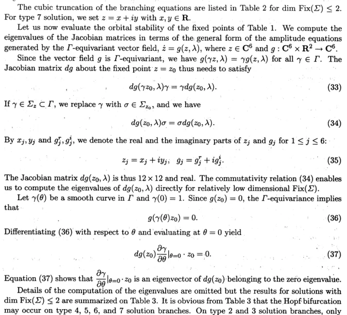
borrowed from [7]

Table 2. Branching equations tmnmted at the cubic order, $\dim$ Fix(\Sigma ) $\leq \mathit{2}$

.

Label Nomenclature Branching equations

2Simple Roll $\sigma 2+\mu 21x^{2}=0$

3SimpleHexagon $\sigma_{2}+\delta_{2}x+(\mu 21+2\mu_{22})x^{2}=0$

4Super Roll $\sigma_{1}+\beta_{1}y+\kappa 11x^{2}+\mu 11y^{2}=0$,

$\sigma_{2}y+\beta_{2}x^{2}+\kappa_{21}x^{2}y+\mu_{21}y^{3}=0$

5Simple Rectangle $\sigma_{2}x+\delta_{2}y^{2}+(\mu 21x^{2}+2\mu 22y^{2})x=0$, $\sigma_{2}+\delta_{2}x+\mu_{22}x^{2}+(\mu_{21}+\mu_{22})y^{2}=0$

6Super Hexagon $\sigma_{1}+\beta 1y+\delta_{1}x+(\kappa 11+2\kappa_{12})x^{2}+(\mu_{11}+2\mu 12+\nu_{1})y^{2}$

$+(2\eta_{1}+\xi_{1})xy=0$,

$\sigma_{2}y+\beta_{2}x^{2}+\delta_{2}y^{2}+(\kappa_{21}+2\kappa_{22}+2\xi_{2})x^{2}y$

$+(\mu_{21}+2\mu_{22})y^{3}+\iota\rho x^{3}=0$

7Thiangle $\sigma 2x+\delta_{2}(x^{2}-y^{2})+(\mu 21+2\mu 22)x^{3}+(\mu 21+2\mu_{22})xy^{2}=0$, $\sigma 2-2\delta_{2}x+(\mu 21+2\mu 22)x^{2}+(\mu 21+2\mu 22)y^{2}=0$

Ifz is apoint of$\mathrm{C}^{6}$, the elementsof$\Gamma$ which leave z fixed form asubgroup of$\Gamma$ called the

isotropy subgroup

or

stabilizer $\Sigma_{z}$ defined by

$\Sigma_{z}=\{\sigma\in\Gamma:\sigma z=z\}$ (29)

The fixed point subspace of asubgroup$\Sigma\subset\Gamma$ is given by

Fix(U) $=$

{

z$\in \mathrm{C}^{6}$ :

$\sigma z=\sigma$ for all $\sigma\in\Sigma$

}.

(30)

Points

on

the

same

orbit of $\Gamma$, i.e., _{$\Gamma z=\{\gamma z : \gamma\in\Gamma, z\in \mathrm{C}^{6}\}$}, have conjugate isotropy

subgroups,

$\Sigma_{\gamma z}=\gamma\Sigma_{z}\gamma^{-1}$

.

(31)

We thus classify the isotropysubgroups up to conjugacy classes.

Table 1lists the fixed points of $g(z, \lambda)=0$ and the isotropy subgroups of $\Gamma$ acting

on

$\mathrm{C}^{6}$

together with theirfixed point subspaces. In the table,

$S^{1}(0, \theta)$ : $(z_{1,2,3,4,5}zzzz, z_{6})arrow(z_{1}, z_{2}\mathrm{e}^{-\dot{l}\theta}, z_{3}\mathrm{e}^{\dot{l}\theta}, z_{4}, z_{5}\mathrm{e}^{-2:\theta}, z_{6}\mathrm{e}^{2_{\dot{l}}\theta})$ ,

$Z_{2}(\pi, 0)$ : $(z_{1}, z_{2}, z_{3}, z_{4}, z_{5}, z_{6})arrow(-z_{1}, -z_{2}, z_{3}, z_{4}, z_{5}, z_{6})$,

$Z_{2}(0,\pi)$ : $(z_{1}, z_{2}, z_{3}, z_{4},z_{5}, z_{6})arrow(z_{1}, -z_{2}, -z_{3}, z_{4}, z_{5}, z_{6})$

.

(32)

There

are

two primary branches, i.e., type 2and 3solutions. The simple roll and simple

hexagonal pattern possess the wavenumber $2\mathrm{k}\mathrm{c}$

.

Since we

assume

the generic situation without

degeneracy, neither the rolls with $k_{\mathrm{c}}$

nor

the hexagons with $k_{c}$ may exist. Four secondary

branches satisfying $\dim$ Fix(\Sigma ) $=2$ may exist; they

are

type 4, 5, 6, and 7solutions. As is

seen

ffom the Table 1, super-rolls

are

composedofrolls with wavenumber $k_{c}$and rolls with $2k_{c}$

.

Likewise, super-hexagons are composed of hexagons with wavenumber $k_{c}$ and hexagons with

$2k_{c}$.

The cubic truncation of the branching equations are listed in Table 2for $\dim$ Fix(F) $\underline{<}2$.

For type 7solution, we set $z=x+iy$ with $x$,$y\in \mathrm{R}$

.

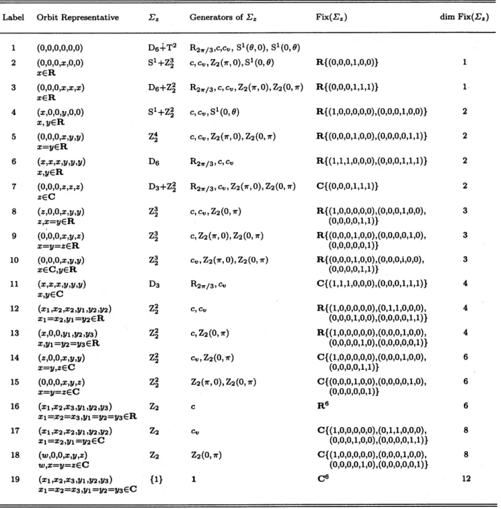
Let us now evaluate the orbital stability of the fixed points of Table 1. We compute the

eigenvalues of the Jacobian matrices in terms of the general form of the amplitude equations

generated by the $\Gamma$-equivariant vector field,

$\dot{z}=\mathrm{g}(\mathrm{z}, \lambda)$, where $z\in \mathrm{C}^{6}$ and$g:\mathrm{C}^{6}\cross \mathrm{R}^{2}arrow \mathrm{C}^{6}$

.

Since

the vector field $g$ is $\Gamma$-equivariant,

we

have _{$g(\gamma z, \lambda)=\gamma g(z, \lambda)$} for all

$\gamma\in\Gamma$

.

The

Jacobian matrix $dg$ about the fixed point _{$z=z_{0}$} thus needs to satisfy

$dg(\gamma z0, \lambda)\gamma=\gamma dg(z_{0}, \lambda)$

.

(33)

If$\gamma$ $\in\Sigma_{z}\subset\Gamma$, we replace $\gamma$ with $\sigma\in\Sigma_{z_{\mathrm{o}}}$, and we have

$dg(z_{0}, \lambda)\sigma=\sigma dg(z_{0}, \lambda)$

.

(34)

By $xj$,$y_{j}$ and $g_{j}^{r}$,$g_{j}^{i}$,

we

denote the real and the imaginary parts of

$z_{j}$ and $g_{j}$ for $1\leq j\leq 6$:

$z_{j}=x_{j}+iy_{j}$, $g_{j}=g_{j}^{r}+ig_{j}^{i}$

.

(35)

The Jacobian matrix $dg(z_{0}, \lambda)$ is thus $12\cross 12$ andreal. The commutativity relation (34) enables

us to compute the eigenvalues of$dg(z_{0}, \lambda)$ directly for relatively low dimensional Fix(F).

Let $\gamma(\theta)$ be asmooth

curve

in $\Gamma$ and _{$\gamma(0)=1$}

.

Since $g(z_{0})=0$, the $\Gamma$-equivariance implies

that

$g(\gamma(\theta)z_{0})=0$

.

(36)

Differentiating (36) with respect to 0and evaluating at $\theta=0$ yield

$dg(z_{0}) \frac{\partial\gamma}{\partial\theta}|_{\theta=0}\cdot z_{\mathrm{O}}=0$

.

(37) Equation (37) shows that $\frac{\partial\gamma}{\partial\theta}|_{\theta=0}\cdot z_{0}$is

an

eigenvectorof

$dg(z_{0})$ belonging to the

zero

eigenvalue.

Detailsof the computation of the eigenvalues

are

omitted but the results for solutions with

$\dim$Fix(I7) $\leq 2$ aresummarizedon Table3. It isobvious from Table 3that the Hopf bifurcation

may

occur

on type 4, 5, 6, and 7solution branches. On type 2and 3solution branches, only

steadybifurcations arise.

Table 4shows the signs of theeigenvalues atthe cubic orderapproximationand eigenvectors

belonging to the eigenvalues for type 2and 3solutions. On the type 2solution branch, type

4solution bifurcates at $\frac{\partial g_{1}^{r}}{\partial x_{1}}=0$ and $\frac{\partial g_{1}^{i}}{\partial y_{1}}=0$, type 5solution bifurcates at $\frac{\partial g_{5}^{r}}{\partial x_{5}}\pm\frac{\partial g_{5}^{r}}{\partial x_{6}}=0$

.

Supercriticality of the type 2solution is guaranteed if $\frac{\partial g_{4}^{r}}{\partial x_{4}}<0$ holds. If $\frac{\partial g_{2}^{r}}{\partial x_{2}}=0$ holds, linear

combinations of the four eigenvectors may create type 12, 13, 16, 17, 18, or 19 solutions in

principle.

Supercriticality of the type 3solution is guaranteed if $\frac{\partial g_{4}^{r}}{\partial x_{4}}+2\frac{\partial g_{4}^{r}}{x_{5}}<0$ holds.

$\mathrm{o}\mathrm{n}\backslash _{\tau}$

the

tyPe 3 solution branch, type 7solution bifurcates at $\frac{\partial g_{4}^{i}}{\partial y_{4}}=0$, type 5solution bifurcates at

$\frac{\partial g_{4}^{r}}{\partial x_{4}}-\frac{\partial g_{5}^{r}}{\partial x_{5}}=0$, type 6and 8solutions may bifurcate at $\frac{\partial g_{1}^{r}}{\partial x_{1}}=0$, and type 11, 12, 14, or 17

solutions may bifurcate at $\frac{\partial g_{1}^{i}}{\partial y_{1}}=0$

.

Note that the orbital stability determined in this paper is with respect to disturbances

supported only by the hexagonal lattice and not by adifferent lattice like the square

or

the

rectangular.

4. Application to $\mathrm{t}\mathrm{w}\mathrm{o}\ovalbox{\tt\small REJECT}$ ayered Rayleigh-Benard convection

4.1. Governing equations and numerical methods

In thissection,

we

applythe aboveanalysesto theRayleigh-Benardconvection composedof

two horizontal fluid layers. They

are

sandwiched between atopand abottom horizontal plates

and ahorizontal ‘splitter plate’ which is non-deformable, conducting, and thin. The bottom

plate is heated and the top plate is cooled at different but uniform temperatures. Because of

the splitter plate, thereis

no

mechanical couplingbetween the upper and the lower fluid layers.

The convection of this type

was

found by Proctor and Jones to have the possibility that the

exact 2:1

resonance

takes place between the critical modes. They analyzed the bifurcation in

one-dimensional 2:1 resonance, indetail, based on the cubically truncated equations (3). In the

one-dimensional pattern formation problem, the cubic amplitude equations describing the 2:1

resonance

(3)

are

generic. However, since the linear operators of the problem, $S$ and $\mathcal{L}$,

are

self-adjoint, the cubic amplitude equations (16)

are

not genericfor two dimensionalpattern

for-mation problem: the coefficients $\delta_{1}$ and$\delta_{2}$ ofthe quadratic nonlineartermsvanish[ll]. In order

to make the cubic equations generic,

we

need to violate theself-adjointnessof the operators. In

this section,

we

do

so

byassumingthe quadratic density profiles

as

functions ofthe temperature.

We take the horizontal $\mathrm{c}\mathrm{o}$-ordinates $x^{*}$ and $y^{*}$, and the vertical $\mathrm{c}\mathrm{o}$-ordinate $z^{*}$ which is

opposite to the direction of the gravity. In what follows, all the asterisked quantities

are

di-mensional. The bottom and the top plates

are

located at $z^{*}=0$ and $d(1+D^{-1})$, _{respectively,}

and the splitter plateis located at $z^{*}=d$

.

The temperatures

on

the bottom and the top plates

are

maintained at $T^{*}=T_{b}$ and $T_{t}^{*}$, respectively. The temperature

on

the splitter plate is at

$T^{*}=T_{m}$.

We attach suffixes 1and 2to indicate variables and physical properties in the lower layer

and the upper layer, respectively. The governingequations for the velocities $\tilde{v_{1,2}}$, the pressures

$p_{1,2}^{*}$, and the temperatures $T_{1,2}^{*}$

are

given by

$\rho_{0}^{(1)}\frac{D\overline{v}_{1}^{*}}{Dt^{*}}=-\nabla^{*}p_{1}^{*}-\rho_{0}^{(1)}g[1-\alpha_{1}^{(1)}(T_{1}^{*}-T_{m})-\alpha_{2}^{(1)}(T_{1}^{*}-T_{m}^{*})^{2}]\mathrm{e}_{z}+\mu_{1}\Delta^{*}\overline{v_{1}}$ ,

$\rho_{0}^{(2)}\frac{D\overline{v}_{\tilde{2}}}{Dt^{*}}=-\nabla^{*}p_{2}^{*}-\rho_{0}^{(2)}g[1-\alpha_{1}^{(2)}(T_{2}^{*}-T_{m})-\alpha_{2}^{(2)}(T_{2}^{*}-T_{m}^{*})^{2}]\mathrm{e}_{z}+\mu_{2}\Delta^{*}\vec{v_{2}}$, $\frac{DT_{1}^{*}}{Dt^{*}}=\kappa_{1}\Delta^{*}T_{1}^{*}$, $\frac{DT_{2}^{*}}{Dt^{*}}=\kappa_{2}\Delta^{*}T_{2}^{*}$,

$\nabla^{*}\cdot\vec{v_{1}}=0$, $\nabla^{*}\cdot\vec{v_{2}}=0$

.

(38)

Here, $g$ is the acceleration due to the gravity, $\mu_{1,2}$

are

the viscous coefficients, $\kappa_{1,2}$

are

the

thermal diffusivities, and $\rho_{0}^{(1)}$ and $\rho_{0}^{(2)}$ arethe densities of the fluids at

$T_{1}^{*}=T_{m}$ and $T_{2}^{*}=T_{m}$,

respectively. In (38), weassumed that the Bussinesq approximation holdsforthe upper and the

lower fluids

so

that the densities only in the buoyancyterms

are

functions of thetemperature.

In the buoyancy terms, $\alpha_{1,2}^{(1)}$ and $\alpha_{1,2}^{(2)}$

are

thermal expansion coefficients. If$\alpha_{2}^{(1)}=\alpha_{2}^{(2)}=0$, the

linear operators

are

self-adjoint.

Let

us now

non-dimensionalize (38) by setting

$t^{*}= \frac{d^{2}}{\kappa_{1}}t,\overline{v_{1}}=\frac{\kappa_{1}}{d}\tilde{v}_{1}$, $\overline{v_{2}}=\frac{\kappa_{1}}{d}\vec{v}_{2}$, $\overline{x}^{*}=d\vec{x}$,

$p_{1}^{*}=-d \rho_{0}^{(1)}g\int^{z}[1-\alpha_{1}^{(1)}(T_{b}-T_{m})(1-z)-\alpha_{2}^{(1)}(T_{b}-T_{m})^{2}(1-z)^{2}]dz+\rho_{0}^{(1)}\frac{\kappa_{1}^{2}}{d^{2}}\pi_{1}$ ,

$p_{2}^{*}=- \dot{d}\rho_{0}^{(2)}g\int^{z}[1-\alpha_{1}^{(2)}(T_{m}-\mathrm{T}\mathrm{t})\mathrm{D}(1-z)-\alpha_{2}^{(2)}(T_{m}-T_{t})^{2}D^{2}(1-z)^{2}]dz+\rho_{0}^{(2)}\frac{\kappa_{1}^{2}}{d^{2}}\pi_{2}$,

$T_{1}^{*}-T_{m}^{*}=(T_{b}-T_{m})[(1-z)+\theta_{1}(x, y, z;t)]$, $z\in[0,1]$,

$T_{2}^{*}-T_{m}^{*}=(T_{m}-\mathrm{T}\mathrm{t})\mathrm{D}(1-z)+\theta_{2}(x, y, z;t)]$, $z\in[1,1+D^{-1}]$

.

(39)

We define non-dimensional parameters by

$R_{1}= \frac{\rho_{0}^{(1)}g\alpha_{1}^{(1)}(T_{b}-T_{m})d^{3}}{\mu_{1}\kappa_{1}}$, $R_{2}= \frac{\rho_{0}^{(2)}g\alpha_{1}^{(2)}(T_{m}-T_{t})d^{3}}{D^{3}\mu_{2}\kappa_{2}}$,

$P_{1}= \frac{\nu_{1}}{\kappa_{1}}$, $P_{2}= \frac{\nu_{2}}{\kappa_{2}}$,

$C_{1}=1$, $C_{2}= \frac{\kappa_{1}}{\kappa_{2}}$, $K_{1}=1$, $K_{2}=D^{4}$, $\epsilon_{1}=\frac{\alpha_{2}^{(1)}(T_{b}-T_{m})}{\alpha_{1}^{(1)}}$, $\epsilon_{2}=\frac{\alpha_{2}^{(2)}(T_{m}-T_{t})D}{\alpha_{1}^{(2)}}$

.

(40)

Following Proctor and Jones,

we

assume

$C_{2}=1$

.

We further set$\overline{T}=1-z$

.

The disturbance

equations in non-dimensional form

are

written

as

$P_{1}^{-1} \frac{D\vec{v}_{1}}{Dt}=-P_{1}^{-1}\nabla\pi_{1}+R_{1}K_{1}\theta_{1}\mathrm{e}_{z}+R_{1}K_{1}\epsilon_{1}(2\overline{T}\theta_{1}+\theta_{1}^{2})\mathrm{e}_{z}+\Delta\overline{v}_{1}$,

$P_{2}^{-1} \frac{D\vec{v}_{2}}{Dt}=-P_{2}^{-1}\nabla\pi_{2}+R_{2}K_{2}\theta_{2}\mathrm{e}_{z}+R_{2}K_{2}\epsilon_{2}(2\overline{T}\theta_{2}+\theta_{2}^{2})\mathrm{e}_{z}+\mathrm{A}\mathrm{v}\mathrm{i}$, $\frac{D\theta_{1}}{Dt}-w_{1}=\triangle\theta_{1}$, $\frac{D\theta_{2}}{Dt}-w_{2}=\Delta\theta_{2}$,

$\nabla\cdot\vec{v}_{1}--0$, $\nabla\cdot\vec{v}_{2}=0$. (41)

Here, $v\mathrm{V}1.2=(u_{1,2}, \mathrm{V}1\cdot 2w_{1,2})^{T}$

.

We impose the boundary conditions

$\vec{v}_{1}=\tilde{v}_{2}=0$ at $z=0,1,1+D^{-1}$,

$\theta_{1}=\theta_{2}=0$ at $z=0,1+D^{-1}$

.

(42)

The boundary conditions at $z=1$ for the temperature

are

imposed by

$T_{1}^{*}=T_{2}^{*}$, $\kappa_{1^{\frac{dT_{1}^{*}}{dz^{*}}}}=\kappa_{2^{\frac{dT_{2}^{*}}{dz^{*}}}}$, (43)

which yield

$\theta_{1}=\frac{R_{2}}{R_{1}}\frac{D^{4}\alpha_{1}^{(1)}\nu_{2}\kappa_{2}}{\alpha_{1}^{(2)}\nu_{1}\kappa_{1}}\theta_{2}\equiv G\theta_{2}$, $\frac{d\theta_{1}}{dz}=G\frac{d\theta_{2}}{dz}$ at $z=1$

.

(44)

Eliminating the pressureterms,

we

obtain the disturbance equations

as

$( \frac{\partial}{\partial t}-P_{j}\triangle)(\frac{\partial v_{j}}{\partial x}-\frac{\partial u_{j}}{\partial y})=\frac{\partial}{\partial x}(\vec{v}_{j}\cdot\nabla)v_{j}-\frac{\partial}{\partial y}(\vec{v}_{j}\cdot\nabla)u_{j}$ ,

$P_{jjjjjjjj2}^{-1_{\frac{\partial\triangle w_{j}}{\partial t}-\triangle^{2}w-RK\Delta_{2}\theta-2\epsilon RK\triangle(\overline{T}\theta)}}j$

$=P_{j}^{-1}[ \frac{\partial^{2}}{\partial x\partial z}(\vec{v}_{j}\cdot\nabla)u_{j}+\frac{\partial^{2}}{\partial y\partial z}(\vec{v}_{j}\cdot\nabla)v_{j}-\triangle_{2}(\vec{v}_{j}\cdot\nabla)w_{j}]+\epsilon_{j}R_{j}K_{j}\triangle_{2}\theta_{j}^{2}$,

$\frac{\partial\theta_{j}}{\partial t}-\Delta\theta_{j}-w_{j}=-(\vec{v}_{j}\cdot\nabla)\theta_{j}$,

$\nabla\cdot\vec{v}_{j}=0$, (45)

where $\triangle_{2}=\frac{\partial^{2}}{\partial x^{2}}+\frac{\partial^{2}}{\partial y^{2}}$ isthe horizontal Laplacian.

Introduce the normal mode

$(u_{j}, v_{j}, w_{j}, \theta_{j})^{T}=(\hat{u}_{j},\hat{v}_{j},\hat{w}_{j},\hat{\theta}_{j})\mathrm{e}^{\sigma t+:(\alpha x+\beta y)}$

.

(46)

The linear eigenvalue problem thus consists of

$P_{j}^{-1}\sigma(i\alpha v_{j}-i\beta uj)-S(i\alpha v_{j}-i\beta u_{j})=0$,

$iauj+iauj+Dwj$ $=0$, $P_{j}^{-1}\sigma Sw_{j}-S^{2}w_{j}+R_{j}K_{j}\gamma^{2}\theta_{j}+2\epsilon_{j}R_{j}K_{j}\gamma^{2}\overline{T}\theta_{j}=0$ , $\sigma\theta_{j}-S\theta_{j}-w_{\mathrm{j}}=0$ (47) under uj $=vj=wj=Dwj$ $=\theta_{j}=0$ at

z

$=0,1+D^{-1}$, uj $=vj=wj=Dwj$ $=0$, $\theta_{1}=G\theta_{2}$, $D\theta_{1}=\mathrm{G}\mathrm{V}\theta 2$ at

z

$=1$

.

(48)

Here, D denotes $\frac{d}{dz}$

.

We solved the linear eigenvalue problem (47) and (48) and corresponding adjoint problem

by means of the expansions in Chebyshev polynomials. The boundary conditions at $z=1$

are

imposed by the tau method. An application of the collocation method yields algebraic

eigenvalueproblems. The QZ package ofIMSL is used to solve theproblems, numerically. First,

we

confirmedthe accuracy ofthe

resonance

conditions which

are

givenin Table1of Proctorand

Jones; i.e., $R_{1}=1401.8$, $r\equiv R_{2}/R_{1}=1.0607$, $k_{c}=\sqrt{\alpha^{2}+\beta^{2}}=2.9150$, and $D=2.0977$for the

linear density profile with $\alpha_{2}^{(1)}=\alpha_{2}^{(2)}=0$

.

In Fig.1,

we

show the linear neutral curves for two

Prandtl numbersets, $(P_{1}, P_{2})=(7,7)$ and (143.759, 7) with various values of$\epsilon_{1}$ and e2. We have

fixed the value of the depth ratio

as

$D=2.0977$which is the

same as

the

one

reportedinProctor

and Jones. The linear neutral stability

curves

exhibit the exact 2:1

resonance.

Two minima

on

the

curves

having wavenumbers in the ratio 2:1 give exactly the

same

critical Rayleigh numbers.

Theexact

resonance

forvarious$\epsilon_{1}$ and62values is not surprising since the

resonance

has already

existed for$\epsilon_{1}=\epsilon_{2}=0$

.

All the eigenfunctions and the adjoint functions

are

normalized such that $\langle\tilde{\psi}_{mn}^{(j)}, S\psi_{mn}^{(j)}\rangle=1$

.

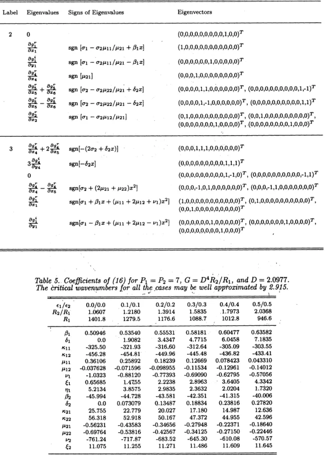
Aftercomputing $\sigma_{mn}^{(j)}$

and $\lambda_{k,l,m-k,n-l}^{(1,p,q)}$ in (12), we evaluated all the coefficients involved in (16)

numerically both for $P_{1}=P_{2}=7$ and $P_{1}=143.759$ and $P_{2}=7$ and tabulated the results in

Table 5and 6, respectively. In the evaluation,

we

assumed that the depth ratio $D$ takes the

value

2.0977.

From

our

numerical data,

we

found that $k_{c}\simeq 2.9150$ gives the 2:1

resonance

for

all the cases shown in the tables. In order to obtain the results,

we

truncated the expansions

in _{Chebyshev polynomials at the 30-th degree and the expansion in the linear eigenfunctions at}

the 20-th.

Since the linear operators involved in

our

problem for $\epsilon_{1}=\epsilon_{2}=0$

are

self-adjoint, the

numerical values of $\delta_{1}$ and $\delta_{2}$ vanish in Tables 5and 6. We may

see

how they recover

non-vanishing values when $\epsilon_{1}$ and $\epsilon_{2}$ deviates from $(0, 0)$

.

Slight increase of the value of

$\epsilon_{2}$

causes

significant effect

on

the non-self-adjointness

4.2. Bifurcation diagrams

Based upon the numerical data of Table 5for $\epsilon_{1}=\epsilon_{2}=0.1$ and Table 6for $\epsilon_{1}=0$ and

e2 $=0.1$, let us examine the bifurcation characteristics of the steady solutions of (16). The

resonance

considered is atw0-parameter bifurcation problem. In our amplitude equations, two

linear growth rates, $\sigma_{1}$ and $\sigma_{2}$

are

formally retained although they

are

assumed to vanish at the

linear criticality. Ingeneral, they depend

on

physical parameters such

as

$R_{1}$, $R_{2}/R_{1}$, Pi, $P_{2}$, $D$,

etc. In the present paper,

we

regard $\sigma_{1}$ and $\sigma_{2}$

as

the bifurcationparameters, for simplicity. Let

us set

$\sigma_{1}=\epsilon\cos\varphi$, $\sigma_{2}=\epsilon\sin\varphi$,

where $\varphi$ lies in $[0, 2\pi]$

.

The modulus $\epsilon$ is set to be 10. This value is so small that the steady

solutions obtained may be considered to be local.

InFigs.2 and 3, onlythe primary and the secondarysolution branches

are

depicted; The

bi-furcationpointsareshown by the closed circlesonthe steadysolutionbrancheswhose$\dim$ Fix(\Sigma )$\leq$

$2$

.

For the stability of each solution branch, see Tables7and 8. The stability assignments ofthe

tablesaresuch that $”+$”denotes apositive eigenvalues, “-,, denotes anegative eigenvalue, _$”**$”

denotes apair of conjugate complex eigenvalues whose real parts are positive, $”==$_”denotes

apair of conjugate complex eigenvalues whose real parts

are

negative, and “0” denotes

azero

eigenvalueforced by the symmetry.

Each entry in Tables 7and 8respectively corresponds to the eigenvalues listed in Table 3.

Sincetheinformation about the multiplicity of adegenerate eigenvalue is involved in Table 3,

we

ignored them in Tables 7and 8. As the primarysolutions, both type 2and 3solutionsbifurcate

from the trivial solution at $\varphi=0$,$\pi$, and $2\pi$, Thetype 2solution exists in$0\leq\varphi\leq\pi$ while the

tyPe 3 solutions exist in $0\leq\varphi\leq\pi$ and $\pi\leq\varphi\leq 2\pi$. Since we

are

looking at the local steady

solutions with small norm, another type 3solution branch with large

norm

does not appear in the

figures although they do exist for $0\leq\varphi\leq 2\pi$. The existence ranges of these primary solutions

are

entirely consistent with the existence ranges of rolls and hexagons in pattern formation

problems without

resonance

(see Fig.la in Buzano and Golubitsky, for instance). Because of

the 2:1 resonant interaction, the third branch of the type 3solutions cannot be stable in both

figures. The stability of the third branch is given by

$”–0-+-$

,, everywhere

as

far as $(\sigma_{1}, \sigma_{2})$

is

in the neighborhood of the origin. The positive eigenvalue $\frac{\partial g_{1}^{r}}{\partial x_{1}}\mathrm{h}\mathrm{s}$ multiplicity three. Table 4

shows that the eigenvectors belonging to $\frac{\partial g_{1}^{r}}{\partial x_{1}}$ involveone of non-vanishing$\mathrm{x}\mathrm{i}$,

$x_{2}$, and $x_{3}$ where

$x_{1}$, $x_{2}$, $x_{3}.\in \mathrm{R}$

.

Let

us now

discuss about the stability of the primary solutions and the secondarybifurcations

from them in Fig.2. Type 2solution is unstable

as

is listed in Table

7.

On the type

2solution

branch, three bifurcation points exist. At the bifurcation points, at least one eigenvalue needs

to change the sign of its real part. For example, the sign of $\frac{\partial g_{1}^{i}}{\partial y_{1}}$ changes at _{$\varphi\simeq 5\cross 10^{-5}\pi$}

at which the stability assignment changes from $2\mathrm{a}$ to $2\mathrm{b}$ with the increase of

$\varphi$

.

By

“$(7\mathrm{c}\mathrm{d})"$,

let us denote abifurcation point at which the stability assignment changes from $7\mathrm{c}$ to $7\mathrm{d}$, for

example, for later convenience. At bifurcation point $(2\mathrm{a}\mathrm{b})$, type 4solution having aproperty

$2\arg(z_{1})-\arg(z_{4})=(2n+1)\pi$, $(n=0, \pm 1, \cdots)$ bifurcates. It vanishes at $\varphi=3\pi/2$

on

the trivial

solution. This corresponds to “$\mathrm{S}_{-}$” of [5] or “$\mathrm{M}_{-}$” of [1] and [10]. At point $(2\mathrm{c}\mathrm{d})$, $\frac{\partial g_{1}^{r}}{\partial x_{1}}$ changes

its sign and another type 4solution with $2\arg(z_{1})-\arg(z_{4})=2n\pi$bifurcates. The latter type

4solution branch vanishes at $\varphi=\pi/2$ on the trivialsolution. It correspondsto “$\mathrm{S}_{+}$”or “$\mathrm{M}_{+}"$

.

At bifurcation point $(2\mathrm{b}\mathrm{c})$, $\frac{\partial g_{2}^{r}}{\partial x_{2}}$ vanishes. This eigenvalue is degenerate with multiplicity four

as has been listed in Table 4. At most four solution branches

are

thus expected to bifurcate; at

this moment, three bifurcating branches

are

identified, i.e., two type 12 solutions and

one

type

13 solution.

On the type 3solution branch, twelve branches bifurcate in total. As is

seen

from Tables

7and 3, $\frac{\partial g_{1}^{r}}{\partial x_{1}}$ changes its sign at $(3\mathrm{a}\mathrm{b})$ and $(3\mathrm{d}\mathrm{e})$ while $\frac{\partial g\mathrm{i}}{\partial y_{1}}$ changes its sign at $(3\mathrm{b}\mathrm{c})$ and $(3\mathrm{e}\mathrm{f})$

.

These eigenvalues

are

degenerate with multiplicity three.

At

most three branches

are

thusexpectedto bifurcate at each

bifurcation

points. Two type

6solutions

and type

12

solution

bifurcate at $(3\mathrm{a}\mathrm{b})$ and $(3\mathrm{d}\mathrm{e})$ whereas type 8, type 11, and type 12 solutions bifurcate at $(3\mathrm{b}\mathrm{c})$

and $(3\mathrm{e}\mathrm{f})$

.

The type 6solutions

are

tw0-dimensional extension oftype 4solutions.

Wehaveidentifiedthe primary and the secondary branchesand examinedtheorbitalstability

of the type 4and 6solutions whose $\dim$ Fix(U)$=$ $2$

.

Although

we

do not involve the detailed

information about the signs ofthe eigenvaluesfor secondary solutions with$\dim$Fix(Il)$\geq$ $3$,

we

needto note thatthey

are

orbitallyunstable. Insummary, onlythe short segment$6\mathrm{i}$’isorbitally

stable.

Figure 3shows similar bifurcation diagram for $P_{1}=143.759$, $P_{2}=7$, $\epsilon_{1}=0$, and $\epsilon_{2}$ $=0.1$

.

For the stability of the primary and the secondary solution branches with $\dim$Fix(\Sigma )$\leq 2$,

see

Table 8. Again, asmall segment

on

the type 6solution is found to be unstable. All the other

primary and the secondarybranches shown in the figure

are

found to be unstable.

References

[1] ArmbrusterD., GuckenheimerJ., P. Holmes, Heteroclinic cycles and modulatedtravelingwavesin

systemswith$\mathrm{O}(2)$ symmetry, Physica D29(1988) 257-282.

[2] E. Buzano, M. Golubitsky, Bifurcation on the hexagonal lattice and the planar Benard problem,

Phil. Trans. R. Soc. Lond. A308 (1983) 617-667.

[3] E.Buzano,A.Russo,Bifurcationproblemswith$\mathrm{O}(2)\oplus \mathrm{Z}_{2}$symmetryand thebucklngof cylindrical

shell, Annuli d:MatematicaPura ed Applicata (IV) 146 (1987) 217-262.

[4] J. Can, Applications

_of

Centre

_Manifold

Theory, (Springer-Verlag, 1981).

[5] G. Dangelmayr, Steady state mode interactionsin presence of$\mathrm{O}(2)$ symmetry, Dyn. Stab. Syst. 1

(1986) 159-185.

[6] K. Fujimura, Centre manifold reduction and the Stuart-Landau equation for fluid motions, Proc.

R. Soc. Lond. A453 (1997) 181-203.

[7] M. Golubitsky, I. Stewart, D.G. Shaeffer, Singularities and Groups in

_Bifurcation

Theory, volume

II, (Springer-Verlag,1988).

[8] M. Golubitsky, J.W. Swift, E. Knobloch,, Symmetries and pattern selection in Rayleigh-Benard

convection, PhysicaD1O (1984) 249-276.

[9] J. Porter, E. Knobloch, Newtype ofcomplex dynamics in the 1:2spatial resonance.

[10] M.R.E. Proctor, C.A. Jones, The interaction of two spatially resonant patterns in thermal convec-tion. Part 1. Exact 1:2 resonance, J. Fluid Mech. 188, (1988) 301-335.

[11] A. Schliiter, D. Lortz, F.H. Busse, On the stabilityof steady finite amplitude convection, J. Fluid

Mech. 23 (1965) 129-144

Table 1. The orbit representatives and the isotropy subgroups

_of

the

_fixed

points under$\mathrm{D}_{6}\dotplus \mathrm{T}^{2}$

Label Orbit Representative $\Sigma_{z}$ Generators of$\Sigma_{z}$ $\mathrm{F}\mathrm{i}\mathrm{x}(\Sigma_{z})$ $\dim \mathrm{F}\mathrm{i}\mathrm{x}(\Sigma_{z})$

1(0,0,0,0,0,0) $\mathrm{D}_{6}\dotplus \mathrm{T}^{2}$

$\mathrm{R}_{2\pi/3},c,c_{v}$,$\mathrm{S}^{1}(\theta,$0), $\mathrm{S}^{1}$(0,

$\theta)$ 2 (O,O,O,x,O,O) $\mathrm{s}^{1}+\mathrm{Z}_{2}^{3}$ c,$c_{v}$,Z2$(\pi,$0),$\mathrm{S}^{1}$(0,

$\theta)$ $\mathrm{R}\{(0,0,0,1,0,0)\}$ 1

$x\in \mathrm{R}$

3 (O,O,O,x,x,x) $\mathrm{D}_{6}+\mathrm{Z}_{2}^{2}$ $\mathrm{R}_{2\pi/3}$,c,$c_{v}$,Z2$(\pi,$0),Z2(0,$\pi)$ $\mathrm{R}\{(0,0,0,1,1,1)\}$ 1

$x\in \mathrm{R}$

4 $(x,\mathrm{O},\mathrm{O},y,\mathrm{O},\mathrm{O})$ $\mathrm{S}^{1}+\mathrm{Z}_{2}^{2}$ $c$,$c_{v}$,$\mathrm{S}^{1}(0, \theta)$ _{$\mathrm{R}\{(1,0,0,0,0,0),(0,0,0,1,0,0)\}$} 2

$x$,$y\in \mathrm{R}$

5 $(\mathrm{O},\mathrm{O},\mathrm{O},x,y,y)$ $\mathrm{z}_{2}^{4}$ $c$,$c_{v}$,$\mathrm{Z}_{2}(\pi, 0)$,$\mathrm{Z}_{2}(0, \pi)$ $\mathrm{R}\{(0,0,0,1,0,0),(0,0,0,0,1,1)\}$ 2

$x=y\in \mathrm{R}$

6 $(x,x,x,y,y,y)$ $\mathrm{D}\epsilon$ $\mathrm{R}_{2\pi/3}$,$c$,$c_{v}$ $\mathrm{R}\{(1,1,1,0,0,0),(0,0,0,1,1,1)\}$ 2 $x,y\in \mathrm{R}$

7 $(\mathrm{O},\mathrm{O},\mathrm{O},z,z,z)$ $\mathrm{D}_{3}+\mathrm{Z}_{2}^{2}$ $\mathrm{R}_{2\pi/3}$,$c_{v}$,Z2$(\pi, 0)$,Z2$(0, \pi)$ $\mathrm{C}\{(0,0,0,1,1,1)\}$ 2 $z\in \mathrm{C}$

8 $(\mathrm{z},\mathrm{O},\mathrm{O},\mathrm{x},\mathrm{y},\mathrm{y})$ $\mathrm{z}_{2}^{3}$ $c$,$c_{v}$,$\mathrm{Z}_{2}(0, \pi)$ $\mathrm{R}\{(1,0,0,0,0,0),(0,0,0,1,0,0)$, 3

$z,x=y\in \mathrm{R}$ (0,0,0,0,1,1)$\}$

9 $(\mathrm{O},\mathrm{O},\mathrm{O},\mathrm{x},\mathrm{y},\mathrm{z})$ $\mathrm{z}_{2}^{3}$ $c$,Z2$(\pi, 0)$,Z2$(0, \pi)$ $\mathrm{R}\{(0,0,0,1,0,0),(0,0,0,0,1,0)$, 3

$x=y=z\in \mathrm{R}$ (0,0,0,0,0,0)$\}$

10 $(\mathrm{O},\mathrm{O},\mathrm{O},\mathrm{x},\mathrm{y},\mathrm{y})$ $\mathrm{z}_{2}^{3}$ $c_{v}$,Z2$(\pi, 0)$,Z2$(0, \pi)$ $\mathrm{R}\{(0,0,0,1,\mathrm{O},0),(0,0,0,\mathrm{i},0,0)$, 3

$x\in C,y\in \mathrm{R}$ (0,0,0,0,1,1)$\}$

11 $(x,x,x,y,y,y)$ D3 $\mathrm{R}_{2\pi/3}$,$c_{v}$ $\mathrm{C}\{(1,1,1,0,0,0),(0,0,0,1,1,1)\}$ 4

$x,y\in \mathrm{C}$

12 $(\mathrm{x}\mathrm{i},\mathrm{x}2,\mathrm{x}3,\mathrm{y}\mathrm{i},\mathrm{y}2,\mathrm{y}3)$ $\mathrm{z}_{2}^{2}$ $c$,$c_{v}$ $\mathrm{R}\{(1,0,0,0,0,0),(0,1,1,0,0,0)$, 4

$x_{1}=x_{2},y_{1}=y_{2}\in \mathrm{R}$ (0,0,0,1,0,0),(0,0,0,0,1,1)$\}$

13 $(x,0,0,y_{1},y_{2},y\mathrm{s})$ $\mathrm{z}_{2}^{2}$ $c$,$\mathrm{z}_{2}(0, \pi)$ $\mathrm{R}\{(1,0,0,0,0,0),(0,0,0,1,0,0)$, 4

$x,y_{1}=y_{2}=y\mathrm{a}\in \mathrm{R}$ (0,0,0,0,1,0),(0,0,0,0,0,1)$\}$

14 $(\mathrm{z},\mathrm{O},\mathrm{O},\mathrm{x},\mathrm{y},\mathrm{y})$ $\mathrm{z}_{2}^{2}$ $c_{v}$,Z2$(0, \pi)$ $\mathrm{C}\{(1,0,0,0,0,0),(0,0,0,1,0,0)$, 6

$x=y,z\in \mathrm{C}$ (0,0,0,0,1,1)$\}$

15 $(\mathrm{O},\mathrm{O},\mathrm{O},x,y,z)$ $\mathrm{z}_{2}^{2}$ Z2$(\pi, 0)$,Z2$(0, \pi)$ $\mathrm{C}\{(0,0,0,1,0,0),(0,0,0,0,1,0)$, 6

$x=y=z\in \mathrm{C}$ (0,0,0,0,0,0)$\}$

16 $(x_{1},x_{2},x3,y_{1},y_{2},y_{3})$ Z2 $c$ $\mathrm{R}^{6}$ 6

$x_{1}=x_{2}=x_{3},y_{1}=y_{2}=y_{3}\in \mathrm{R}$

17 $(\mathrm{x}\mathrm{i},\mathrm{x}2,\mathrm{x}2,\mathrm{y}\mathrm{i},\mathrm{y}2,\mathrm{y}2)$ Z2 $c_{v}$ $\mathrm{C}\{(1,0,0,0,0,0),(0,1,1,0,0,0)$, 8

$x_{1}=x_{2},y_{1}=y_{2}\in \mathrm{C}$ (0,0,0,1,0,0),(0,0,0,0,1,1)$\}$

18 $(w,\mathrm{O},\mathrm{O},x,y,z)$ Z2 Z2$(0, \pi)$ $\mathrm{C}\{(1,0,0,0,0,0),(\theta,0,0,1,0,0)$, 8

$w,x=y=z\in C$ (0,0,0,0,1,0),(0,0,0,0,0,1)$\}$

19 $(x_{1},x2,x3,y_{1},y2,y\mathrm{a})$ {1} 1 $\mathrm{C}^{6}$ 12

$x_{123}=x=x,y_{1}=y_{2}=y_{3}\in \mathrm{C}$

Table 3. Eigenvalues

_of

the Jacobian matrices

_for

the$prima\eta$ and the secondary solutions.

Label Eigenvalues Multiplicity

1 $\mathrm{a}\mathrm{e}_{1}^{\mathrm{L}}\partial g^{r},$ $\neq_{x_{4}}^{\partial g^{r}}$ 6,6

2 0, $\frac{\partial}{\partial}\mathit{9}^{r}\lrcorner x_{1}’\neq_{\mathrm{V}1}^{\partial g}.\cdot’\neq_{x_{4}}^{\partial g^{r}}$ 1,1,1,1 $\frac{\partial}{\partial}\mathit{9}^{r}x_{5}\Delta$_$+$$\mathrm{f}\mathrm{f}_{0}^{r}\partial g$, $\mathrm{f}^{\mathit{9}}\mathrm{f}_{\epsilon}^{r}-^{\partial}\partial\epsilon_{0}^{\mathit{9}^{r}}$ 2,2

$\neq_{x_{2}}^{\partial g^{r}}$ 4

3 $H_{4}+2\#_{x\mathrm{g}’}3\dot{P}_{4}\partial g^{r}\partial g^{r}\partial g$

.

1,1

$0,$ $\neq_{x_{4}}^{\partial g^{r}}-\partial H_{\epsilon}^{\mathit{9}^{r}}$ 2,2

$\mathrm{a}\mathrm{e}_{1}^{\mathrm{L}}\partial g^{r},$ $\tau_{\nu 1}\partial g_{[perp]}.\cdot$ 3,3

4 0, $\frac{\partial g\mathrm{i}}{\partial_{\mathrm{V}1}}+\neq_{\mathrm{V}4}\partial g.\cdot$ 1,1 $\epsilon_{l}^{\partial g^{r}}-\partial H_{\epsilon}^{\mathit{9}^{r}}’\not\in_{5}^{\partial g^{r}}+^{\partial g}\mathrm{f}\mathrm{f}_{\mathrm{o}’}^{r}\mathrm{a}_{2}^{r}\partial-^{\partial}\#_{x_{3}}^{\mathit{9}^{r}},$ $\neq_{x_{2}}^{\partial g^{r}}+\neq_{x_{3}}\partial_{\mathit{9}^{r}}$ 2,2,2,2

$\lambda_{1}^{(4)},\lambda_{2}^{(4)};\lambda_{1}^{(4)}+\lambda_{2}^{(4)}=\mathrm{t}\mathrm{r}A$, $\lambda_{1}^{(4)}\lambda_{2}^{(4)}=\det A$, $A=(^{\partial g}\partial\not\in^{r}1e_{1}^{s^{r}}$ $\mathrm{a}\mathrm{e}_{\alpha)}^{\mathrm{L}}g_{4}\partial g^{r}\partial g^{r}$ 1,1

5 $\epsilon_{1}^{\partial g^{r}}$, $\dot{\mathrm{g}}_{\mathrm{V}1}^{\partial g},$ $\neq_{\mathrm{V}4}^{\partial g}.\cdot+2_{T_{\mathrm{V}\epsilon}}^{\partial g\mathrm{i}}$, $\mathrm{f}g\mathrm{f}_{5}^{r}-\partial\partial\neq_{x_{0}}g^{r}$ 1,1,1,1

$0,$ $\neq_{x_{2}}^{\partial g^{r}}’\neq_{\nu 2}^{\partial g}.\cdot$ 2,2,2

$\lambda_{1}^{(5)},\lambda_{2}^{(5)};\lambda_{1}^{(5)}+\lambda_{2}^{(5)}=\mathrm{t}\mathrm{r}A$, $\lambda_{1}^{(5)}\lambda_{2}^{(5)}=\det A$, $A=(_{\not\in}^{\partial g^{r}}\partial\neq_{x_{4}}g^{r}‘$ $\frac{\partial g_{5}^{r}2}{\partial x_{5}}+\not\in_{l}H_{5}^{\partial g^{r_{\partial g^{r)}}}}$ 1,1

6 $0,$ $\neq_{\mathrm{V}4}^{\partial_{\mathit{9}}}.\cdot-\partial\dot{\phi}^{\mathit{9}}$

.

$+^{\partial}\neq_{\mathrm{V}1}^{\mathit{9}}‘-\partial\dot{*}g$ .

2,2

$\lambda_{1}^{(6)},\lambda_{2}^{(6)}j\lambda_{1}^{(6)}+\lambda_{2}^{(6)}=\mathrm{t}\mathrm{r}A$, $\lambda_{1}^{(6)}\lambda_{2}^{(6)}=\det A$, $A=(_{\vec{\partial x_{1}}}^{\partial}\mathrm{a}^{\mathit{9}_{\mathrm{L}^{\partial g^{r}}}}\mathrm{e}_{1}^{r}\dagger 2\partial\partial g^{r}\neq_{x_{2}}g^{r}\not\in_{2}+2$ $\not\in_{4}^{\partial g^{4}}+2\neq_{x_{5}}^{x_{4)}}\not\in_{r}^{\partial_{\mathit{9}^{r}}}+2\neq\partial g^{r}\partial g^{r}$ 1,1

$\lambda_{1}^{\prime\langle 6)},\lambda_{2}^{\prime(6)};\lambda_{1}^{\prime(6)}+\lambda_{2}^{\prime(6)}=\mathrm{t}\mathrm{r}B$, $\lambda_{1}^{\prime(6)}\lambda_{2}^{\prime(6)}=\det B$, $B=(_{\neq}^{\neq}$$\partial g\partial g^{}\nu 1u.1^{\cdot}+2^{\partial g}+2\dot{\neq}_{\mathrm{V}2}\neq_{\mathrm{V}2}\partial g.\cdot$. $\neq_{\mathrm{V}4}^{\partial g}.\dot{.}.+2^{\partial g^{l}}\neq_{\mathrm{V}4}^{\partial g}+2\frac{\neq_{\mathrm{V}4}\partial g_{4}}{\partial y\mathrm{g}}\dot{.}$

)

1,1

$\lambda_{1},\lambda_{2}j\lambda_{1}+\lambda_{2}^{\prime\prime(6)}=\mathrm{t}\mathrm{r}C\prime\prime(\epsilon)\prime\prime(6)\prime\prime(\epsilon)$, $\lambda_{1}^{\prime\prime(6)}\lambda_{2}^{\prime\prime(6)}=\det C$, $C=(_{\neq}^{\partial}\not\in\partial_{\mathit{9}^{r},x_{1}}^{1}\mathit{9}^{r}-\partial\neq_{x_{2}}-^{\partial}\neq_{x_{2}}^{g^{r}}g^{r}$ $\not\in_{4}g^{r}-\partial\partial\neq_{*\epsilon}\not\in_{4}g^{r}-\partial\partial\neq_{x_{4}}g^{r}g^{r})$ 2,2

7 $0,$ $\not\in_{4}^{\partial_{\mathit{9}^{r}}}-\partial_{\mathit{9}^{r}}\neq_{x_{8}}+^{\partial}*_{4}^{\mathit{9}}\cdot$

.

$-^{\partial}\dot{\mu}_{\nu s}^{\mathit{9}}$

.

2,2

$\lambda_{1}^{(7)},\lambda_{2}^{(7)}j\lambda_{1}^{(7)}+\lambda_{2}^{(7)}=\mathrm{t}\mathrm{r}A$, $\lambda_{1}^{(7)}\lambda_{2}^{(7)}=\det A$, $A=(^{\partial}$$\mathrm{f}\#\mathrm{f}\partial gx_{1}\mathit{9}^{r}.!$ $\neq_{\nu_{!}}^{\partial g^{r}}\hslash_{1}\partial g\mathrm{i}$

)

3,3

$\lambda_{1}^{\prime(7)},\lambda_{2}^{\prime(7)};\lambda_{1}^{\prime(7)}+\lambda_{2}^{\prime(7)}=\mathrm{t}\mathrm{r}B$, $\lambda_{1}^{\prime(7)}\lambda_{2}^{\prime(7)}=\det B$, $B=(_{\neq}^{\partial}$$\not\in\partial g*_{4}\cdot\cdot\neq_{x\epsilon}^{x_{8}}\mathit{9}^{r}4+2+2\neq\partial g^{r}\partial g.\cdot$ $\neq_{l4}^{\partial_{\mathit{9}^{r}}}+2*_{\epsilon}\neq_{\nu 4}^{\partial g^{j}}+2_{\hslash \mathrm{s}}^{\partial g_{\dot{\mathrm{A}}}}\partial g^{r}$.

)

1,1

Table

_4.

Eigenvalues, signs

_of

the eigenvalues at the cubic order approximation, and eigenvectors

_of

the Jacobian matnces_forthe primar$ry$ solutions.

Label Eigenvalues Signs of Eigenvalues Eigenvectors

20 $(0,0,0,0,0,0,0,0,0,1,0,0)^{T}$

$Tx_{1}\partial g^{r}[perp]$

$\mathrm{s}\mathrm{g}\mathrm{n}[\sigma_{1}-\sigma 2\mu 11/\mu 21+\beta_{1}x]$ $(1,0,0,0,0,0,0,0,0,0,0,0)^{T}$

$\frac{\partial g}{\partial y}i1$ sgn_{$[\sigma_{1}-\sigma_{2}\mu_{11}/\mu_{21}-\beta_{1}x]$} $(0,0,0,0,0,0,1,0,0,0,0,0)^{T}$ $\vec{\partial x_{4}}\partial g^{r}$ sgn$[\mu_{21}]$ $(0,0,\mathrm{Q},1,0,0,0,0,0,0,0,0)^{T}$

$\neq_{x_{5}}^{\partial g^{r}}+\mathrm{f}\mathrm{f}_{6}^{r}\partial g$ sgn $[\sigma_{2}-\sigma_{2}\mu 22/\mu_{21}+\delta_{2}x]$ $($0,0,0,0,1,1,0,0,0,0,0,0$)^{T}$, $(0,0,0,0,0,0,0,0,0,0,1,- 1)^{T}$ $\neq_{x\mathrm{s}}^{\partial g^{r}}-\frac{\partial g}{\partial x}\mathrm{A}r6$

$\mathrm{s}\mathrm{g}\mathrm{n}[\sigma_{2}-\sigma_{2}\mu 22/\mu 21-82\mathrm{x}]$ $($0,0,0,0,1,-1,0,0,0,0,0,0$)^{T}$, $(0,0,0,0,0,0,0,0,0,0,1,1)^{T}$ $\neq_{x_{2}}^{\partial g^{r}}$ sgn $[\sigma_{1}-\sigma_{2}\mu_{12}/\mu_{21}]$ $($0,1,0,0,0,0,0,0,0,0,0,0$)^{T}$,$($0,0,1,0,0,0,0,0,0,0,0,0$)^{T}$,

$($0,0,0,0,0,0,0,1,0,0,0,0$)^{T}$, $(0,0,0,0,0,0,0,0,1,0,0,0)^{T}$

3 $\neq_{x_{4}}^{\partial g^{r}}+2^{\partial g^{r}}\neq_{x_{5}}$ $\mathrm{s}\mathrm{g}\mathrm{n}[-(2\sigma_{2}+\delta_{2}x)]$ $(0,0,0,1,1,1,0,0,0,0,0,0)^{T}$ $3^{\partial}\neq_{v4}^{\mathit{9}}$

.

$\mathrm{s}\mathrm{g}\mathrm{n}[-\delta_{2}x]$ $(0,0,0,0,0,0,0,0,0,1,1,1)^{T}$

0 $(\mathrm{o},\mathrm{o},\mathrm{o},\mathrm{o},\mathrm{o},\mathrm{o},\mathrm{o},\mathrm{o},\mathrm{o},1,- 1,0)^{T}$, $(0,0,0,0,0,0,0,0,0,0,- 1,1)^{T}$

$\neq_{x_{4}}^{\partial_{\mathit{9}^{r}}}-\partial\neq_{x_{5}}g^{r}$ $\mathrm{s}\mathrm{g}\mathrm{n}[\sigma_{2}+(2\mu_{21}+\mu_{22})x^{2}]$ $($0,0,0,-1,0,1,0,0,0,0,0,0$)^{T}$,$(0,0,0,- 1,1,0,0,0,0,0,0,0)^{T}$ $Tx_{1}\partial g^{r}[perp]$ $\mathrm{s}\mathrm{g}\mathrm{n}[\sigma_{1}+\beta_{1}x+(\mu_{11}+2\mu_{12}+\nu_{1})x^{2}]$

$(0,0,1,0,0,0,0,0,0,0,0,0)^{T}(1,0,0,0,0,0,0,0,0,0,0,0)^{T}$,

$($0,1,0,0,0,0,0,0,0,0,0,0$)^{}$ , $\tau_{\nu 1}^{i}\partial g$ $\mathrm{s}\mathrm{g}\mathrm{n}[\sigma_{1}-\beta_{1}x+(\mu_{11}+2\mu_{12}-\nu_{1})x^{2}]$

$(0,0,0,0,0,0,0,0,1,0,0,0)^{T}(0,0,0,0,0,0,1,0,0,0,0,0)^{T}$, $(0,0,0,0,0,0,0,1,0,0,0,0)^{T}$,

$\underline{-}$

$\beta_{1}$ 0.50946 0.53540 0.55531 0.58181 0.60477 0.63582 $\delta_{1}$

a.o

1.9082 3.4347 4.7715 6.0458 7.1835 $\kappa_{11}$ -325,50 -321.93 -316,60 -312.64 -305.09 -303.55 $\kappa_{12}$ -456.28 -454.81 -449.96 -445.48 -436.82 -433.41 $\mu 11$ 0.36106 0.25892 0.18239 0.12669 0.078423 0.043310 $\mu 12$ -0.037628 -0.071596 -0.098955 -0.11534 -0.12961 -0.14012 $\nu_{1}$ -1.0323 -0.88120 -0.77393 -0.69090 -0.62795 -0.57056 $\xi_{1}$ 0.05685 $\mathrm{X}.4\mathrm{Z}55$ 2.2238 2-89633.6405 4.3342 $\eta_{1}$ 5.2134 3.8575 2.9835 2.3632 2.0204 1.7320 $\mathrm{A}$ -45.994 -44.728 -43.581 -42.351 -41.315 -40.006 $\delta_{2}$ 0.0 0.073079 0.13487 0.18834 0.23816 0.27820 $\kappa_{21}$ 25.755 22.779 20.027 17.180 14.987 12.636 $\kappa_{22}$ 56.318 52.918 50.167 47.372 44.955 42.596 $\mu_{21}$ -0.56231 -0.43583 -0.34656 -0.27948 -0.22371 -0.18640 $\mu 22$ -0.69764 -0.53816 -0.42567 -0.34125 -0.27150 -0.22446 $\nu_{2}$ -761.24 -717.87 -683.52 -645.30 -610.08 -570.57 $\xi_{2}$ 11.075 11.255 11.271 11.486 11.609 11.645

$\overline{-}$

93

$ble\dot{T}h_{6C\sqrt}ticalwavenumbersfor\theta Coefficientsof(\mathit{1}\mathit{6})forP_{2}allthe\omega ses=7,G=1$, $D=may2.0977beweli$$a_{\mathrm{P}proximate^{2}\mathit{4}_{by^{1}\mathit{2}.\mathit{9}\mathit{1}\mathit{5}}^{R\cross D^{4}}}andP_{1}--R$.

$\overline{-}$

$\mathrm{e}\mathrm{i}/\mathrm{e}2$ 0.0/0.0 0.0/0.1 0.0/0.2 0.0/0.3 0.0/0.4 0.0/0.5 $R_{2}/R_{1}$ 1.0607 1.11234 1.1692 1.2321 1.3021 1.3804 $R_{1}$ 1401.8 1400.8 1399.7 1398.6 1397.2 1395.8 – $\beta_{1}$ -1.5978 -1.5598 -1.5164 -1.4661 -1.4064 -1.3370 $\delta_{1}$ 0.0 0.31158 0.64348 1.0199 1.4455 1.9311 $\kappa_{11}$ -319.66 -315.87 -311.79 -307.36 -302.54 -297.27 -771.86 -791.31 -809.36 -824.62 -838.78 -84.40 $\kappa_{12}$ -26.736 -29.365 -32.340 -35.707 -39.531 -43.929 $\mu 11$ -143.74 -160.03 -178.36 -199.44 -223.55 -251.95 $\mu 12$ $\nu_{1}$ -211.99 -237.02 -265.09 -297.54 -334.76 -379.45 $\xi_{1}$ -192.77 -205.77 -217.74 -229.10 -239.03 -246.97 -507.01 -566.82 -631.31 -703.72 -784.94 -879.81 $\eta_{1}$ $\beta 2$ 152.01 166.49 182.28 199.63 218.81 240.17 $\delta_{2}$ 0.0 1.6948 3.5814 5.6928 8.0661 10.767 $\kappa_{21}$ 351.80 502.46 678.13 884.41 1129.0 1420.8 7284.3 8763.7 10562 12787 15553 19058. $\kappa_{22}$ -252.58 -261.98 -272.64 -284.59 -297.86 -312.95 $\mu 21$ -309.28 -319.17 -330.24 -342.38 -355.55 -370.12 $\mu 22$ 47825 58205 70887 86592 106410 131410 $w$ $\xi_{2}$ 5738.9 6953.5 8454.0 10329 12698 15705

$\overline{-}$

$R_{1}$ $k$

Fig.1. Linearneutral stabilty

curves.

$D=2.0977$,

Fig.2. Bifurcation diagram for Table 5, $\epsilon 1=\epsilon_{2}=0.1$

.

Fig.3. Bifurcationdiagram for Table 6, $\epsilon_{1}=0$, $\epsilon_{2}=0.1$