PERIODIC SOLUTIONS FOR FORCED VAN DER POL TYPE EQUATIONS (Mathematical Economics : Dynamic Macro-economic Theory)

PERIODIC

SOLUTIONS

FOR

FORCED

VAN

DER

POL

TYPE

EQUATIONS

CHIKAHIRO

EGAMI

AND

NORIMICHI

HIRANO

ABSTRACT. In the presentpaper,wewillseethataVan der Pol type equations has aperiodic

solution when theforcing term is periodic. By showing the results ofsomesimulations,we

illustrate periodicityofthe solutions. Wealso provethat aperiodic solution found nearthe

origin is arepellor. Key Words

Van der Pol type equation, Forcing term, Periodic solution, Banach space, Topological

(Leray-Schauder) degree, Repellor, Attractor, Subharmonic solution

1INTRODUCTION

Let $f$,$g$,$e:\mathrm{R}$$arrow \mathbb{R}$ becontinuous functions. The Lienard typeequation with forcing term

(L) $u_{tt}+f(u)u_{t}+g(u)=e(t)$ $t\in \mathrm{R}$

has been studied by many authors due to its adoption to awide variety of mechanical,

electrical, biological and economical systems. The equation (L) is usually called Duffing

type when $f(u)=\langle$,orVander Pol type when $g(u)=\eta u$, where $\langle$ and$\eta$

are

constants.

In economics, there have been anumber of elegant mathematical treatments of

some

of the traditional business cycle theories e.g. the treatment of Kaldor’s model by Chang

andSmyth (1971) andSchinasi (1982) andofacomplete Keynesian system byTorre (1977).

Becauseof

one

dimensional relaxation oscillatorjustlikeVanderPol typewithoutanforcing

term, their treatments concentrated

on

the question of the existence of limit cycles and

consequently made

use

of the planar properties such

as

Poincare-Bendixson theory and

Jordan curve (cf. C. Chiarella [14, \S 2, \S 3,

\S 7],

K. Kawamata [15, pp.131-148]).

Recently, $N$-dimensional extension of the equation (L) has been studied by several

au-that However it is not easy for $N\geq 2$ to obtain similar results as

one

dimensional

cases.

$N$-dimensionalexistence results forperiodicsolutions oftheforced Van der Poltype

are

not

yet established until

now

in comparison with those of the forced Duffingtype (e.g.,

see

[1]

by J. Mawhin).

Throughout this paper,unless otherwiseexplicitly stated,$F$,$g:\mathrm{R}^{N}arrow \mathrm{R}^{N}$

a

$\mathrm{e}$continuous

functions,and$e\in L^{2}(\mathbb{R};\mathbb{R}^{N})$isaperiodicfunctionwithperiod$T$

.

We consider theexistence

problem forperiodicsolutions of the forced$N$-dimensional Van der Poltypeequationof the

form

(V) $u_{tt}+ \frac{d}{dt}F(u)+g(u)=e(t)$ $t\in \mathrm{R}$,

where $u(t)=(u_{1}(t),u_{2}(t)$,$\ldots$ ,$\mathrm{u}(\mathrm{t})$, and $u:(t)\in \mathbb{R}$ for each $t\in \mathrm{R}$ and each integer

$i\in[1, N]$

.

In the following section,

we

shall prove our main result for (V). We make

use

of the

Leray-Schauder degree theory(cf. N. G. Lloyd [12,

\S 4],

K. Masuda[21, \S 23,

\S 24]).

Insection

数理解析研究所講究録 1264 巻 2002 年 159-172

3,

we

give the results of the simulations

for

some

concrete models. In section 4,

we

prove

that the periodic solution found

near

the origin by simulations in section3is repellor.

2EXISTANCE

OF

PERIODIC

SOLUTIONS

In this section,

we

establish

an

existence result for periodicsolutions

of

(V). To state

our

result,

we

need

some

preliminaries.

For$x,y$$\in L^{2}([0,\eta j\mathrm{R}^{N})$, let

us

definethat

$|x|$ $=( \sum_{=1}^{N}x_{}^{2)^{1/2}},$ $||x||=( \int_{0}^{T}|x(t)|^{2}dt)^{1/2}$, $(x,y)$ $= \int_{0}^{T}.\sum_{\Leftarrow 0}^{N}x:(t)y_{\dot{*}}(t)dt$

.

Inthe folowing,

we

put

$H=\{u\in L^{2}([0,T]j\mathrm{R}^{N}):"(0)=u(T),u_{t}\in L^{2}([0,T];\mathrm{R}^{N})\}$,

with the

norm

$||u||_{H}=(||u||^{2}+11\mathrm{u}11^{2})^{1/2}$

Wealso put

$\tilde{H}=\{u\in H:\int_{0}^{T}u(t)dt$ $=0\}$

.

Further,$\dot{g}\mathrm{v}\mathrm{e}\mathrm{n}$ aset $\Omega$,itsclosure is written$\overline{\Omega}$

, its boundary$\partial\Omega$

.

Our

mainresult is thefollowing,

Theorem 2.1 Let

e

$\in H$

.

If

$F(u)$ and$g(u)$ satisfy the

follow

.ng

conditions (Fl), (F2) and

(Gl), then the$d|.ffe|\mathrm{e}nt|.al$ equation (V) has atleast

one

periodic solution with period T.

(F1) $F(u_{1},u_{2}, \ldots,u_{N})=(\begin{array}{l}F_{1}(u_{1})F_{2}(u_{2})\vdots F_{N}(u_{N})\end{array})$ ,

where $F_{}\in C^{1}(\mathrm{R};\mathrm{R})$

for

each integer:$\in[1, N]j$

(F2) $f_{}(0)<0$ and $\lim_{[\cdot 1arrow}\inf_{\infty}\frac{f_{}(s)}{s^{2}}>0$,

where $f_{}$ denotes$F_{j}’$

(G1) $g(u)=Au$ and $\det A\neq 0$,

$whm$ $A$ _is a$N\mathrm{x}N$ constant matrix.

To prove Theorem 2.1

we

need

some

lemmata. However,

we

omit thoseproofs here.

Lemma 2.2 Suppose that(Fl), (F2) and (Gl). Let

e

$\in H$

.

If

$u(t)$ is

a

T periodic solution

of

the

_differential

equation (V), thenu $\in\tilde{H}$ and

$||u||\leq 2T||u_{t}||$

.

Remark. For the inequality in Lemma 2.2, whichiscalled Poincare’s inequality,

we

can

have

still stricter evaluation (cf. C. P. Gupta, J. J. Nieto and L. Sanchez [3]). However, the

present evaluation is enough for lemmata in this paper.

Lemma 2.3 Let$\lambda_{0}\in(0, \min(_{\mathrm{T}}^{2\pi}, 1))$

.

Then the set

$S_{1}= \{u\in H:u_{tt}+\frac{d}{dt}F(u)+\lambda Au=e(t)$

for

some

A$\in[\lambda_{0},1]\}$

is bounded in$H$

.

Lemma 2.4 The set

$S_{2}=\{u\in H$: $u_{tt}+ \delta\frac{d}{dt}F(u)+\mathrm{X}$ Au$=6e(t)$

for

some

$\delta$_$\in[0,1]\}$

is bounded in $H$

.

Here, let

us

introduce the topological (Leray-Schauder) degreeand its properties. Definition 2.5 LetX be Banachspace, $D$ beabounded opensubset_$ofX$ and$\mathcal{L}$be

a

compact

mapping from $\overline{D}$ into X.

If

$\mathcal{L}x\neq p$

for

any $x\in\partial D$, then we

define

the Leray-Schauder degree

_of

$\mathcal{L}$ at

$p\in X$ relative to $D$ to be $\deg(\mathcal{L}, D,p)$

.

The Leray-Schauder degree is known to have the following three properties.

(i) $\deg(I, D,p)=1$ for every$p\in D$, where I denotes identity mapping,

(ii) $\deg(\mathcal{L}, D,p)\neq 0$ implies $\mathcal{L}x=p$forsome $x\in D$

.

(iii) If$\mathcal{H}(\xi)$ is ahomotopyofcompact mapping with $\mathcal{H}(\xi)x\neq p$for any $x\in\partial D$ and any

$\xi\in[0,1]$,then $\deg(\dot{\mathcal{H}}(\xi), D,p)$ isindependent of$\langle$

.

Proof of Theorem 2.1 Let $B_{r}(0)$ be the open ball in $\tilde{H}$

centered at 0with radius$r$ $>0$

.

For each$\lambda\in[0,1]$ and$\delta\in[0,1]$,

we

defineaoperator$\mathcal{T}(\lambda, \delta)$ :$\tilde{H}arrow\tilde{H}$ by

$\mathcal{T}(\lambda,\delta)u=-\delta\int_{0}^{t}F(u(s))ds-\lambda\int_{0}^{t}\int_{0}.Au(\tau)d\tau ds+\delta\int_{0}^{t}\int_{0}.e(\tau)d\tau ds+C$,

where

$C= \delta\int_{0}^{T}F(u(s))ds+\lambda\int_{0}^{T}\int_{0}^{\epsilon}$ Au(r)$d \tau ds-\delta\int_{0}^{T}\int_{0}^{e}e(\tau)d\tau ds$

.

Because $\mathcal{T}(\lambda, \delta)$ is aintegral operator, $\mathcal{T}(\lambda, \delta)U$ is equicontinuous for any bounded subset

$U$ of$\tilde{H}$

.

Then $\mathrm{T}(\mathrm{A}, \delta)U$is relatively compact by Ascoli-Arzela theorem. Hence $\mathcal{T}(\lambda, \delta)$ is

a

compact operator. Furthermore,

we

put

$\mathcal{H}(\xi)u=\{$

$\mathcal{T}(1-3(1-\lambda_{0})\xi, 1)u$ for $\xi\in[0, \frac{1}{3}]$ and$u\in\tilde{H}$,

$\mathcal{T}(\lambda_{0},2-3\xi)u$ for$\xi\in[\frac{1}{3}, \frac{2}{3}]$ and $u\in\tilde{H}$,

$\mathrm{T}(3\mathrm{A}\mathrm{O}(1-\xi), \mathrm{O})u$ for$\xi\in[\frac{2}{3},1]$ and $u\in\tilde{H}$

.

Then $\mathcal{H}(\xi)$ is ahomotopy ofcompact mapping

on

$\tilde{H}$

.

It is obvious from the definition of

$\mathcal{H}(\xi)$ that _$u$ is afixed points of$\mathcal{H}(0)$ if and only if$u$ is asolution of (V). We have by the

definition of$?t(\xi)$ that

$S_{1}=\{u\in\tilde{H}$ : $u=\mathcal{H}(\xi)u$ for

some

$\xi\in[0, \frac{1}{3}]\}$

$S_{2}=\{u\in\tilde{H}$ :$u=\mathcal{H}(\xi)u$ for

some

$\xi\in[\frac{1}{3}, \frac{2}{3}]\}$

.

Then by

Lemma

2.3

andLemma 2.4,

we

have that there exists large$M_{0}$ such that

$u\neq \mathcal{H}(\xi)u$ for any$u\in\partial B_{M_{0}}(0)$ andany $\xi$$\in[0, \frac{2}{3}]$

.

For$\langle$$\in[\frac{2}{3},1]$,

we can see

thateach fixed point$u\in\tilde{H}$of$\mathcal{H}(\xi)$ satisfies

(2.1) $u=-(3 \lambda_{0}(1-())\int_{0}^{t}\int_{0}.$ $\mathrm{v}(\mathrm{t})$$d\tau ds$$+C$

.

Then

we

immediatelyhave that $u=0$isthe unique solutionof (2.1),

we

also have that

$u\neq \mathcal{H}(\xi)u$ for any$u\in\partial B_{M_{0}}(0)$ andany$\xi\in[\frac{2}{3},1]$

.

While,

we

should just calculate $\deg(I-\mathcal{H}$(0)$, B_{M_{0}}(0),0)$ to consider the fixed point

problem $u=\mathrm{H}(0)$

.

Since

$u\neq \mathcal{H}(\xi)u$for any$u\in\partial B_{M_{\mathrm{Q}}}(0)$and any $\xi\in[0,1]$, then by the

property (iii) of degree,

$\deg(I-\mathcal{H}(0),B_{M_{0}}(0),\mathrm{O})=\deg(I-\mathcal{H}(1),B_{M_{0}}(0),\mathrm{O})=\deg(I,B_{M_{0}}(0),0)$

.

Using the property (i) of degree, $\deg(I,Bu_{0}(0),0)=1$

.

Therefore by the property (\"u) of degree,

we

obtain that$H(0)$ has at least

one

fixed point in$\tilde{H}$, and Theorem

2.1 is proved.

$\mathrm{O}$

3VAN

DER

POL

OSCILLATOR

Insection 3, We showed existence of periodic solution of(V). Then

we

would like tofindout whereaperiodic solution with period$T$ exits. In this section,

we

introduce three concrete examples and illustrate the results of simulationsfor each model.

3.1

PRELIMINARY

Wedefine three kinds ofperiodic solutions with mutuallydifferent character.

Definition 3.1 Letu $\in L^{2}([0,T]jR^{N})$ be aperiodicsolution with periodT

of

(V).

If

there

exists aneighborhood U

_of

$\Gamma=\{(u(t),u_{t}(t));$t$\in[0,T]\}$ such that

$\lim_{tarrow+\infty}d((v(t),v_{t}(t))$,$\Gamma)=0$

for

each $(v_{0},v_{t0})\in U$,

where $v(t)$ is a solution

of

(V) with initial value $(\mathrm{v}(0),\mathrm{v}\mathrm{t}(\mathrm{O}))=(\mathrm{v}0\mathrm{i}\mathrm{v}\mathrm{t}0)\in R^{N}\mathrm{x}R^{N}$ and

$d(\cdot$,$\cdot$$)$ denotes usualEuclid distance, then_$u$ is said to be attractive or attractor.

Definition 3.2 In contrast

_of

_Definition

31,

_if

there $\dot{\varpi}stsU$

of

$\Gamma$ such that

$\lim_{tarrow-\infty}d((v(t),v_{t}(t))$,$\Gamma)=0$

for

each $(v_{0},v_{t0})\in U$, then$u$ is saidto be repellor.

Definition3.3

_If

$u$ is a periodic solution with the integral multiple

of

$T$, then $u$ is said to

be subharmonic solution

3.2

NORMAL

MODEL

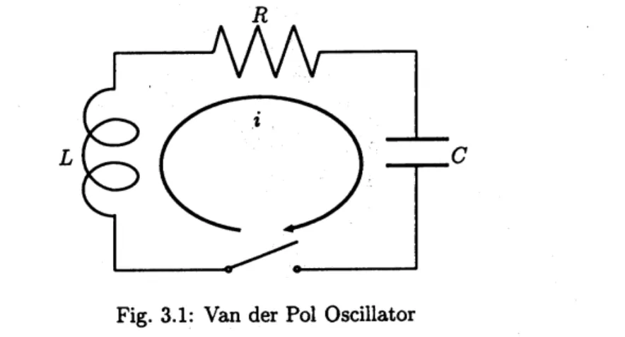
We first introduce the most basic oscillating circuit with anegative resistor devised by

Van der Pol. On Fig.3.1, $L$, $C$ and $R$ stands for inductance, capacitance and resistance,

$L$

Fig. 3.1: Van der Pol Oscillator

respectively. This$R$, iscalled negativeresistor,hasthe nonlinear property forcurrent $i$such

that

(3.1) $R(i)=-\prime 0+r_{1}i$_%$r_{2}i^{2}$,

where$r_{0}$,$r_{1}$ and$r_{2}$ isnonnegative. Let$\tau$ be time. Thenthecircuit equation corresponding

toFig.3.1 is formalized by thefollowing

$Li_{\tau}+R(i)i+ \frac{1}{C}\int i(\tau)d\tau=0$

.

Differentiating above equation by $\tau$, wehave

$i_{\tau\tau}- \frac{1}{L}(r_{0}-2\mathrm{r}\mathrm{x}\mathrm{i}-3r_{2}i^{2})i_{\tau}+\frac{1}{LC}i=0$

.

Here, transforming $\tau$ into $\sqrt{LC}t$ andputting $i=\sqrt{\overline{3}r_{2}\prime[perp]}x$,

we

have

(3.2) $x_{tt}-r_{0} \sqrt{\frac{C}{L}}(1-\frac{2r_{1}}{\sqrt{3r_{0}r_{2}}}x-x^{2})xt+x=0$

.

Put $\epsilon=\prime_{0}\sqrt{\frac{c}{L}}$

now.

If

we

suppose_{$r_{1}=0$}, then

we

obtain the Van der Poltypeequation

(M1) $x_{tt}+\epsilon(x^{2}-1)\mathrm{x}\mathrm{t}+x=0$,

where $x(t)\in \mathrm{R}$

.

$\epsilon$ represents the nonlinearity of the system (M1) and (3.1) holds the

essence

of Self-induced oscillation. In

case

that $\epsilon$ is equal to zero, (M1) is actually just

a

linear oscillator. Itisknownasarelaxation oscillation that the solutions oftheautonomous

system (M1) have the unique limit cycle for each$\epsilon$

on

$(x,x_{t})$ plane by Poincare-Bendixson

Theorem (cf. F. Verhulst [10,

\S 4.3]).

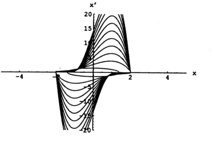
Fig.3.2 gives the $\omega$-limit set of the orbits. Where

$\epsilon$ change from 0to 20 by 2step. The horizontal axis and the vertical axis indicates $x(t)$

and $x_{t}(t)$, respectively. We

can see

in Fig.3.2 the amplitude of limit cycle becomes large

as

$\epsilon$ grows. For example, the period of limit cycle for $\epsilon=2,\epsilon=6.5$ and

$\epsilon$ $=15$ is about

7.63, 13.79and 26.80

$\mathrm{x}’$

$\mathrm{x}$

Fig.

3.2:

Limit Cycle

3.3

FORCED MODEL

We next introduce the Van der Pol oscillator withexternalpower

source.

On

Fig.3.3, $E$is

thevoltageof externalpower

source.

Using transformationsimilar to(3.2),

we can

formulate

the circuit equation_{corresponding toFig.3.3}

_as

_follows

(3.3) $x_{tt}-r_{0} \sqrt{\frac{C}{L}}(1-\frac{2r_{1}}{\sqrt{3r_{0}r_{2}}}x-x^{2})x_{t}+x=\sqrt{\frac{3r_{2}}{r_{0}}}\sqrt{\frac{C}{L}}E\mathrm{c}\mathrm{o}\mathrm{e}t$

Weput$\epsilon=r_{0}\sqrt{\tau c}$and$B=\sqrt{\underline{3}\mathrm{a}\mathrm{o}},\sqrt{\tau c}E$

.

Wecall$B$forcing coefficient. If

we

assume

_{$r_{1}=0$},

thenwehave the forced Van der Poltype equation

(M2) $x_{tt}+\epsilon(x^{2}-1)x_{\mathrm{C}}+x=B$

coe

$t$

.

We show three results of simulations of the model (M2). Then

we

have to set

a

initial value

on

$[0, 2\pi]$ $\mathrm{x}\mathrm{R}^{N}\mathrm{x}\mathrm{R}^{N}$

.

Let

us

set four initial values $(t_{0},x(t_{0}),x_{t}(t_{0}))$ at

(0,0,0), (0,0,3),$(0,$_{$-1, 1)$}and (0, 1,5). Let $\epsilon$ be fixed at 10.0 and $B$ be set at 2.0, 6.5

Fig.3.3: Van der Pol Oscillatorwith External power

source

and 15.0. It is rather

more

important for

us

than the relation between initial values and

orbits whether aperiodic solution exists

or

where aperiodic solution

was

observed

or

its

period. Fig.3.4, Fig.3.5 and Fig.3.6

are

3-dimensional plots and projections onto $t=0$ of

time series of$x$ and $x_{t}$ of (M2) in

case

that the amplitude of external force $B$ is weak 2.0,

strong 15.0 and middle 6.5, respectively. In Fig.3.4,

we can

find

a

$2\pi$-periodic repellor in

the region of$t<0$ which oscillate

near

the origin with small amplitude, and

a

$6\pi$ periodic

subharmonicsolution in the region of$t>0$in which allfourorbitsreach. InFig.3.5,

we can

observe

a

$2\pi$-periodic attractor in the region of$t>0$in which allfour orbits

was

attracted

as

time progresses. In the region of$t<0$,

we can

hardly calculatebecausetheorbits diverge

instantly to infinityforall fourinitial values. Fig.3.6 gives acomplicatedstatethat

we

have

arepellor in the region of$t<0$ and both

an

attractor and asubharmonic solution in the

region of$t>0$

.

$\mathrm{x}$ Fig. 3.5: Caseof$B=2$ $\mathrm{x}$ Fig. 3.5: Caseof$B=15$ $\mathrm{x}$ Fig. 3.6: Case of$B=6.5$

165

Fig.3.7andFig.3.8

are

drawn in order to give clearly the orbitsofthree periodic solutions. Fig.3.7 is the 3-dimensional plotof$(t\mathrm{m}\mathrm{o}\mathrm{d} 2\mathrm{n}\mathrm{l}\mathrm{x}(\mathrm{t})\mathrm{J}\mathrm{x}\mathrm{t}(\mathrm{t}))$for large $|t|$sufficiently,and Fig.3.8 is its projection onto $t=0$

.

In Fig.3.8,

we

can

see

that the oscillation with the smallest amplitude is repellor, the orbit is attractor which oscillate by the inner side of the largest

swing, and the orbit issubharmonic solution which also has the small amplitude crossing$x$

axis while oscillating with the largest amplitude.

$\mathrm{x}$

Fig. 3.7: InvariantSet for $|t|>>1$ Fig. 3.8: Periodic Solutions

In Fig.3.9, Fig.3.10 and Fig.3.11, $(t\mathrm{m}\mathrm{o}\mathrm{d} T,x(t))$

are

drawn for $t$ $\in[1W,20]$, $t\in$

$[100,200]$ and$t\in[-2W, -1\mathrm{M}]$ to investigate the exact periodsofperiodicsolutions, where

$T=2\pi,2\pi$ and $6\pi$, respectively. In order to get the exact period,

we

have to choose $T$

appropriately sothat the

curves

$(t \mathrm{m}\mathrm{o}\mathrm{d} T,x(t))$ may be overlapped atone.

$\mathrm{t}$ $\mathrm{t}$

Fig. 3.9: Repellor Fig. 3.10: Attractor

$\mathrm{x}$

$\mathrm{t}$

Fig. 3.11: Subharmonic Soluti

on

3.4

COUPLED MODEL

WITH

FORCING

TERM

We introduce the coupling model connected two oscillating circuits with external power

source.

Fig. 3.12: Coupled VanderPol Oscillator withExternal power

source

On the Fig.3.12, $c$ and $r$ represents the small capacitance added artificially and the

minuteresistance included in the leadportionof the circuit, respectively. Thecharacteristic

ofnegativeresistance is described by

$R_{n}(i)=-\mathrm{r}\mathrm{n}\mathrm{O}+rnli+r_{n2}i^{2}$ for $n=1,2$

.

Now

assume

$\sqrt{L_{1}C_{1}}=\sqrt{L_{2}C_{2}}$and put $i_{1}=\sqrt{3r_{12}r}" x$ and $i_{2}=\sqrt{\frac{r}{3}r_{22}2\mathrm{L}}y$

.

By using

same

transformation as (3.3), we havethe following circuit equation corresponding to Fig.3.12

$x_{tt}-r_{10} \sqrt{\frac{C_{1}}{L_{1}}}(1-\frac{2r_{11}}{\sqrt{3r_{10}r_{12}}}x-x^{2})x_{t}+x=\sqrt{\frac{3r_{12}}{r_{10}}}\sqrt{\frac{C_{1}}{L_{1}}}E_{1}\cos t$

$+ \frac{C_{1}}{c}(y-x)+r\sqrt{\frac{C_{1}}{L_{1}}}(y_{\mathrm{C}}-x_{t})$,

$y_{tt}-r_{20} \sqrt{\frac{C_{2}}{L_{2}}}(1-\frac{2r_{21}}{\sqrt{3r_{20}r_{22}}}y-y^{2})y_{t}+y=\sqrt{\frac{3r_{22}}{r_{20}}}\sqrt{\frac{C_{2}}{L_{2}}}$

a

_{$\cos t$}

$+ \frac{C_{2}}{c}(x-y)+r\sqrt{\frac{C_{2}}{L_{2}}}(x_{\ell}-y_{t})$

.

Here we put $k_{n}=\mathrm{C}\mathrm{n}/\mathrm{c}$, $\epsilon_{n}=r_{n0}\sqrt{\frac{c}{L_{\mathrm{n}}}}$ and $B_{n}=\sqrt{\frac{3}{r}\underline{r_{\mathrm{B}0}}l}\sqrt{\frac{c}{L_{n}}}E_{n}$

.

If

we

suppose

$r_{n1}=0$,

$r\langle(1$, then

we

can build up

our

main model

$x_{tt}-\epsilon_{1}(1-x^{2})x_{t}+x=B_{1}\cos t+k_{1}(y-x)$,

(M3)

$y_{tt}-\epsilon_{2}(1-y^{2})y_{t}+y=B_{2}\cos t+k_{2}(x-y)$,

where

we

call $k_{n}$ couplingcoefficient.

We show two results of simulations of the model (M3). Then

we

have to set ainitial

value

on

$[0, 2\pi]$$\mathrm{x}\mathrm{R}^{N}\mathrm{x}\mathrm{R}^{N}\mathrm{x}\mathrm{R}^{N}\mathrm{x}\mathrm{R}^{N}$

.

Let

$\epsilon_{1}$,$\epsilon_{2}$ and $k_{1}$,$k_{2}$ befixedat 2.0,10.0 and 0.5, 0.3,

respectively. We suppose $B_{1}=B_{2}$

.

We first show

case

ofweak external force $B_{1}=B_{2}=1.5$

.

Let

us

set four initial

val-ues

$(t_{0},x(t_{0}),x_{\ell}(t_{0}),y(t_{0}),y_{(}t_{0}))$ at (0,0,0,0,0), $(0, 0,$$-1, 0,$$-1)$, $(0,$$-2,$ $-5,$ $-1,$$-10)$ _and

$(0,$-2,$5,$-2.5,-10$)$

.

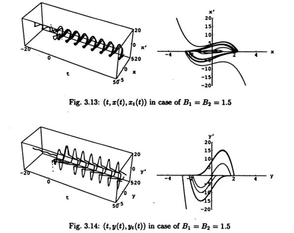
Fig.3.13 and Fig.3.14

are

time series plotting $(t,x(t),x_{t}(t))$ and $(t,y(t),y_{t}(t))$,

respec-tively. In both Fig.3.13 and Fig.3.14,

we

can

observe

a

$2\pi$-periodic repellor in the region

of$t<0$ and

a

$6\pi$-periodic subharmonic solution in the region of$t>0$

.

Then _$x(t)$ of this

subharmonic solution in Fig.3.13

appears

like $2\pi$-periodic. But watching _$y(t)$ in Fig.3.14,

we

have itsperiod is$6\pi$

.

Furthermore,

we

expectthat,

even

if amodel

was

multidimensionalize, theamplitude_of

eachvariabledepend

on

$\mathcal{E}$

:of

each dimension. In this case, the amplitudeof$x(t)$ and$y(t)$

depend

on

$\epsilon_{1}$ and $\epsilon_{2}$, respectively. However, if

we

suppose that coupling coefficients

4is

larger,then

we

may have

amore

complicated situation of the orbits.

$\mathrm{x}$

Fig. 3.13: $(t,x(t),x_{l}(t))$ in

case

of$B_{1}=B_{2}=1.5$

$\mathrm{y}$

Fig. 3.14: $(t,y(t),y_{t}(t))$ in

case

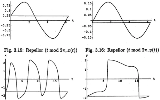
of$B_{1}=B_{2}=1.5$

Fig.3.15, Fig.3.16 and Fig.3.17 Fig.3.18 give theperiodofrepellorand subharmonicsolution,

respectively. We

can

checkthat each periodis $2\pi$ and$6\pi$

.

We next show

case

ofstrongexternalforce $B_{1}=B_{2}=15$

.

Let

us

set fourinitialvalues

$(t_{0},x(t_{0}),x_{t}(t_{0}),y(t_{0})$,$y_{t}(t_{0}))$ at (0,0, 0, 0,0), $(0,$$-2,$ $-5,$ $-1,$$-10)$, $(0,$-2,$5,$-2.5,-10$)$ and

$(0, 3,$$-1, 3, 1)$

.

In Fig.3.19 and Fig.3.20,

we can

observe

a

$2\pi$-periodic attractor in the region of_$t>0$

like$B=15$ of

case

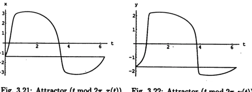
in the last section.In the region of$t<0$, the orbits diverge instantly to

infinityfor all four initial values.Fig.3.21 andFig.3.22givethe periodofattractor is $2\pi$

.

In the end, by the results of

some

simulations,

we can

expect that forced Van der Pol

systemhas

an

attractorin

case

that theexternalforce isstrong

or

arepellorin

case

that the

externalforce is weak. But it is noteasytoinvestigate completely setting ofparameters for

$\mathrm{t}$ $\mathrm{t}$

Fig. 3.15: Repellor $(t\mathrm{m}\mathrm{o}\mathrm{d} 2\pi,x(t))$ Fig.

3.16:

Repellor $(t\mathrm{m}\mathrm{o}\mathrm{d} 2\pi, y(t))$

$\mathrm{x}$ $\mathrm{y}$

t $\mathrm{t}$

Fig. 3.17: Subharmonic(t$\mathrm{m}\mathrm{o}\mathrm{d} 6\pi,x(t)$ Fig. 3.18: Subharmonic(t$\mathrm{m}\mathrm{o}\mathrm{d} 6\pi,y(t)$)

$\mathrm{x}$

Fig. 3.19: $(x(t),x_{t}(t))$ in

case

of$B_{1}=B_{2}=15$

$\mathrm{y}$

Fig. 3.20: $(y(t),y_{\mathrm{C}}(t))$ in

case

of$B_{1}=B_{2}=15$

$\mathrm{y}$

$\mathrm{t}$

$\mathrm{t}$

Fig. 3.21: Attractor$(t\mathrm{m}\mathrm{o}\mathrm{d} 2\pi,x(t))$ Fig. 3.22:

Attractor

$(t\mathrm{m}\mathrm{o}\mathrm{d} 2\mathrm{n}\mathrm{t}\mathrm{y}\{\mathrm{t}))$

all

cases

that asubharmonic solution exists (e.g. _{regarding the results for}

_one

_dimensional

system,

see

J. E. Flaherty and F. C.Hoppensteadt [2]$)$

.

4REPELLOR

In this section ,

we

prove that theperiodic solution found

near

the originbysimulations in

section 3isrepellor.

Proposition 4.1 Let$\rho$be asmall constant, $u\in L^{2}(R;R^{N})$ be

a

$T$-periodicsolution

of

(V)

utsth $||u||\leq\rho$ and$A$ _is

a

Hermite conjugate matrix. Then

$u$ is a repellor.

Proof.

Usingcondition (F2),

we

have that,there exists$\rho:>0$for $:\in[1,N]$ such that

$f\dot{.}(u:)<0$ for $|u:|<\rho:$,

then put $\rho=\mathrm{n}\cdot \mathrm{n}:\epsilon[1,N1$$\rho:$

.

Putting

$f(u)=(\begin{array}{llll}f_{1}(u_{1}) 0 00 f_{2}(u_{2}) 0\vdots \vdots \ddots \vdots 0 0 f_{N}(u_{N})\end{array})$ ,

we can

rewrite (V) to

(4.1) _{$u_{tt}+f(u)u_{t}+Au=e(t)$}

_.

Let $u\in L^{2}(R_{j}R^{N})$ be

a

$T$_periodic solution of (4.1) with _{$||u||\leq\rho$}

.

Further _{let $h$ be}

a

constant and$u+h\phi$ beasolution (4.1). Then

we

_have

(4.2) _{$(u+h\phi)_{tt}+f(u+h\phi)(u+h\phi)_{t}+A(u+h\phi)$ $=e(t)$}

_.

By (4.1) and (4.2),

we

have

$\phi_{tt}+\frac{f(u+h\phi)-f(u)}{h\phi}u_{t}\phi+f(u+h\phi)\phi_{t}+A\phi=0$

.

By letting $h$ _g0to 0forthe equation above,

we

get the linearized

equation

(4.3) $\phi_{tt}+f(u)\phi_{t}+(f’(u)u_{t}+A)\phi=0$,

where$f’(u)$ is Hessian of$f(u)$

.

Here

we

_{rewritetheequationabove}

_as

_{asystemoffirstorder}

ordinary equations of the form

(4.4) $(\begin{array}{l}\phi_{l}\chi_{t}\end{array})=(\begin{array}{ll}0 1-f’(u)u_{\mathrm{C}}-A -f(u)\end{array})(\begin{array}{l}\phi\chi\end{array})$

We consider the initial value problem of autonomous system (4.4) with $(\phi(0), \chi(0))=$

$(00, \chi_{0})\in \mathrm{R}^{N}\mathrm{x}\mathrm{R}^{N}$

.

We put _{$\Phi(t)=(\phi(t), \chi(t))$} for $t\geq 0$

.

Then by Floquet’s theorem

(e.g.,

see

[9,

\S 1.4]

by F. C. Hoppensteadt),

we

have that the fundamental solution $\Phi(t)$ of

(4.4)

can

be written in the form

$\Phi(t)=Q(t)\exp(\Lambda t)$,

where$Q(t)=\{q_{j}\}$ is amatrix such that each element $\mathrm{q}\mathrm{i}\mathrm{j}\{\mathrm{t}$)is

a

$T$-periodic function, and A

is aJordan matrix. To prove that $u$ isarepellor, it is sufficient to

see

that each eigenvalue

$\lambda_{:}$ of Ais positive. Let

$\varphi$ isasolution of (4.3). Then

we

have

$\varphi_{tt}+f(u)\varphi_{t}+(f’(u)u_{t}+A)\varphi=0$

.

Integrating the equation above

over

$[0, t]$,

we

have

$\varphi_{t}(t)+(f(u)\varphi)(t)+A\int_{0}^{t}\varphi(s)ds=\varphi_{t}(0)+(f(u)\varphi)(0)$

Here

we

put $\sigma=\varphi_{t}(0)+(f(u)\varphi)(0)$

.

We alsoput $\phi(t)=\int_{0}^{t}\varphi(s)ds$

.

Then

we

have

$\psi_{tt}+f(u)\psi_{t}+A\psi=\sigma$ for t $\geq 0$

.

Then multiplyingthe equality above by$\psi_{t}$ and integrating

over

$[0, t]$,

we

get

(4.5) $| \psi_{t}(t)|^{2}+(\langle A\psi(t),\psi(t)\rangle\rangle\geq|\psi_{t}(0)|^{2}+(\langle A\psi(0),\psi(0))\rangle+\frac{1}{2}\int_{0}^{t}|\psi_{t}(s)|^{2}ds+\langle\langle\sigma,\psi(t)-\psi(0)\rangle)$

.

where

we

put ($\langle x, y\rangle\rangle=\sum_{=1}^{N}.\cdot x:y$

:for

$x$,$y\in \mathrm{R}^{N}$

.

Suppose that there exists anegative eigenvalue $\lambda_{:}$ ofA. Then by choosing the initial value $(\varphi(0), \varphi_{t}(0))$ appropriately, we have

thatforsome $D>0$,

$|\psi_{t}|\leq De^{\lambda:t},|\psi|\leq De^{\lambda:t}$ for all t $\geq 0$

.

This implies that $\lim_{tarrow\infty}|\psi_{t}(t)|^{2}+\langle\langle A\psi(t),\psi(t)\rangle\rangle=0$and $\lim_{tarrow\infty}\langle\langle\sigma,\psi(t)-\psi(0))\rangle=0$

.

This contradicts to (4.5). This completes the proof. $\square$

REFERENCES

[1] Jean Mawhin, An Extension

_of

a Theorem

_of

A.C.Lazeron Forced Nonlinear

Oscilla-tions, Journal of MathematicalAnalysis and Applications, Vo1.40,pp.20-29, (1972).

[2] J.E.Flaherty, F.C.Hoppensteadt, Frequency Entrainment

_of

a Forced van der Pol

Os-cillator, Studies in Applied Mathematics, Vo1.58, pP.5-15, (1978).

[3] Duane W.Storti, Per G.Reinhall, Stability

_of

in-phave and out-Of-phase modes

_for

$a$

pair

_of

linearly coupled vander Pol oscillators, Nonlinear dynamics, PP.1-23, Series

on

Stability, Vibration and Control Systems. Series B, Vo1.2, World Scientific Publishing,

River Edge, NJ, (1997).

[4] Nguyen PhuongC\’ac, Periodic Solutions

_of

a Li\’enardequation with forcing term, Non-linear Analysis, Vo1.43, pp.403415, (2001).

[5] Chaitan P.Gupta, Juan J.Nieto, LuisSanchez, PeriodicSolutions

_of

Some Lienard and

Duffing Equations,Journal of Mathematical Analysis and Applications,Vo1.140,

PP.67-82, (1989).

[6]

Norman

Levinson, A Second Order

_Differential

Equation with Singular Solutions, An-nalsofMathematics, Vo1.50, No.1, pp.127-153, (1949).

[7] M.L.Cartwright,J.E.Littlewood, SomeFo.eed Point Theorems, Annals of Mathematics,

V01.54, NO.1, pp.1-37, (1951).

[8] John Guckenheimer, Philip Holmes, “Nonlinear Oscillations, Dynamical Systems,and

Bifurcations ofVector Fields”, Applied Mathematical Sciences, 42,

Springer-Verlag,

(1983).

[9]

Frank

C.

Hoppensteadt, “Analysisand

Simulation

ofChaoticSystms” , Applied

Math-ematical Sciences, 94,Springer-Verlag, (2000).

[10] _{Ferdinand Verhulst “Nonlinear Differential Equations and Dynamical Systems”,}

Springer-Verlag, (1990).

[11] Wolfgang Walter uOrdinary Differential Equations

n,

Springer-Verlag,

(1998).

[12] N.G.Lloyd, “Degree Theory”, Cambridge UniversityPress, (1978).

[13] G.Hardy, J.E.Littlewood, G.P61ya, “INEQUALITIES”, Cambridge University Press,

(1934).

[14] _{Carl Chiarella, “The Elements of aNonlinear Theory of Economic Dynamics”,}

Lec-tureNotae in

Economics

and Mathematical Systems, 343, Springer-Verlag, (1990).

[15] Toru Maruyama, Wataru Takahashi, uNoffiinear and Convex Analysis in Economic

$\mathrm{T}\mathrm{h}\infty \mathrm{r}\mathrm{y}"$,LectureNotesinEconomicsandMathematical Systems,419,

Springer-Verlag, (1995).

[16] GianniRicci, KumaraswamyVelupillai, “Growth Cycles andMultisectoral Economics:

the Goodwin Tradition”, LectureNotesin Economics andMathematical Systems, 309,

Springer-Verlag, (1988). [17] 宮寺功, u 関数解析”,理工学社, (1972). [18] 青木利夫, 高橋渉, 平野載倫, u演習集合位相空間”, 培風館, (1985). [東] 浅田統一郎, u成長と循環のマクロ動学” , 日本経済評論社, (1990). [20] 佐藤力, u 非線形振動論$n$ , 基礎物理科学シリーズ, 2, 朝倉書店, (1970). [21] 増田久弥, u非線形数学”, 新数学講座, 15, 朝倉書店, (1985).

CHIKAHIRO

EGAMI\dagger _{AND NORIMICHI} $\mathrm{H}\mathrm{I}\mathrm{R}\mathrm{A}\mathrm{N}\mathrm{O}^{\mathit{1}}$

Division ofInformationMedia Environment Sciences,

Graduate SchoolofEnvironment and InformationSciences,

YokohamaNational University,

795 Tokiwadai, Hodogaya,Yokohama, Kanagawa,

2408501

E-mail address: \dagger chika@hiranolab_{.jks.ynu.ac.jp, hirano@math sci.ynu.ac.jp}