Mean-square stability of numerical schemes for stochastic differential systems (Discretization Methods and Numerical Algorithms for Differential Equations)

(1)

Mean-square stability of numerical schemes

for stochastic differential systems

齋藤善弘 (岐阜聖徳学園大学)

YOSHIHIRO SAITO (Gifu Shotoku Gakuen University)

三井斌友 (名古屋大学)

TAKETOMO MITSUI (Nagoya University) Abstract

Stochastic differential equations (SDEs) represent physical phenomena dominated

by stochastic processes. As for deterministic ordinary differential equations (ODEs),

various numericalschemes areproposed forSDEs. We have proposed the mean-square

stability of numerical schemes for ascalar SDE, that is, the numerical stability with

respect to the mean-squarenorm. However we studied itfor onlyscalar SDEs because

of difficulty and complexity in SDE systems. In the present note we will consider a

2-dimensional linear system with one multiplicative noise andtry to analyze them.

1Introduction

We have proposed the numericalmean-square stability ($\mathrm{M}\mathrm{S}$-stability)for ascalar stochastic

differentialequation (SDE) with

one

multiplicative noise [7]. However

we

studied it for only

scalar SDEs. Komori and Mitsui $[4, 5]$ analyzed numerical $\mathrm{M}\mathrm{S}$-stability for a2-dimensi0nal

SDE with special case, that is, simultaneously diagonalizable

case.

In this note

we

$\mathrm{w}\mathrm{i}\mathrm{U}$ try

to analyze numerical $\mathrm{M}\mathrm{S}$-stability of the Euler-Maruyama scheme for general 2-dimensi0nal

SDE systems.

Consider the SDE ofItO-type given by

$\mathrm{d}X(t)=f(t,X)\mathrm{d}t+g(t,X)\mathrm{d}W(t)$ (1)

with $f(0,t)=g(0, t)=\mathrm{O}$ so that the steady state _$X(t)=0$ is the equilibrium solution. The

Euler-Maruyama scheme for the discrete approximate solution $\{\overline{X}_{n}\}$ is

$\overline{X}_{n+1}=\overline{X}_{n}+f(t_{n},\overline{X}_{n})h+g(t_{n},\overline{X}_{n})\Delta W_{n}$

where $h$ and $\Delta W_{n}$ stand for the step-size and the increment of the Wiener process,

respec-tively. Then

we can

give the definition of the MS-stability.

Definition 1Steady solution $X(t)\equiv \mathrm{O}$ is asymptotically stable in mean-square

if

$\forall\epsilon>0,$ $\exists\delta>0$; E_{$(||X(t)||^{2})<\epsilon$}

for

all t $\geq 0$ and $||X_{0}||<\delta$

and

$\exists\delta_{0}$;

$\lim_{tarrow\infty}$E $(||X(t)||^{2})=0$

for

all $||X_{0}||<\delta_{0}$

数理解析研究所講究録 1265 巻 2002 年 89-99

(2)

Here the

norm

$||x||$ is the Euclidean

norm

of avector $x\in \mathbb{R}^{2}$

.

We willconsider three types of linear SDE systems, and try to analyzethem. In the next

section

we

describe the results of $\mathrm{M}\mathrm{S}$-stabilty for three types ofthe SDE system.

Section

3shows theresults of numerical $\mathrm{M}\mathrm{S}$-stability of the Euler-Maruyama scheme corresponding

to results in Section 2. In Section 4we $\mathrm{w}\mathrm{i}\mathrm{U}$ show the numerical experiments confirming

our

stability analysis in Section

3.

FinaUy

we

$\mathrm{w}\mathrm{i}\mathrm{U}$ describe

our

conclusion andfuture aspects.

2MS-stability

We will restrict the SDE (1) to

an

$\mathrm{I}\mathrm{t}\mathrm{t}\succ \mathrm{t}\mathrm{y}\mathrm{p}\mathrm{e}$ $2$-dimensional lnear SDE system with

one

multiplicative noise, which has the form

$\{$

$\mathrm{d}X(\mathrm{t})$ $=DX(t)\mathrm{d}\mathrm{t}+BX(\mathrm{t})\mathrm{d}W(\mathrm{t})$,

$X(0)$ $=$ $1$. (2)

Here the real constant matrices $D$ and $B$

are

given by

$D=\{\begin{array}{ll}\lambda_{1} 00 \lambda_{2}\end{array}\}$ , $B=[_{\beta_{2}}\alpha_{1}$ $\alpha_{2}\beta_{1}]$

.

Komori and Mitsui $[4, 5]$ analyzed $\mathrm{M}\mathrm{S}$-stabilty for SDE system (2) with

$\beta_{1}=0$ and $\beta_{2}=0$ (simultaneously diagonalizable case). We $\mathrm{w}\mathrm{i}\mathrm{U}$ consider

more

general SDE system,

namely $\beta_{1}\neq 0$ and $\beta_{2}\neq 0$

.

First

we

$\mathrm{w}\mathrm{i}\mathrm{U}$ introduce the conventional and the logarithmic

norms

of matrices for stability analysis ofthe SDE system (2).

Definition 2Corresponding to the vector

norms

$l^{1},$ $l^{2}$ and $l^{\infty}$ in $\mathrm{R}^{n}$, we

define

the

setbor-dinate $mat\dot{m}$

nors

of

square $n\cross n$ matrix $A=(a_{1j}.)$ by

$||A||_{1}= \max_{j}\{\sum_{=1}^{n}.\cdot|a_{j}.\cdot|\}$ , $||A||_{\infty}= \max.\cdot\{\sum_{j=1}^{n}|a_{j}.\cdot|\}$ ,

$||A||_{2}=$ $\{$maximum eigenvalue

of

$A^{T}A\}^{1/2}$

Definition 3Logarithmic rnatrixnorm $\mu[A]$ (see [1, $\mathit{6}J$) is

defined

by

$\mu[A]=\lim_{harrow 0+}(||I+hA||-1)/h$

where I is the unit matrix and h $\in \mathrm{R}$

.

For the matrix

norms

$||\cdot||_{1},$ $||\cdot||_{\infty}$ and $||\cdot||_{2}$, the folowing identities

are

well known to

evaluate the logarithmic

norms.

$\mu_{1}[A]=\max_{j}\{a_{jj}+\sum_{\neq \mathrm{j}}.\cdot|a_{j}.\cdot|\}$ , $\mu_{\infty}[A]=\mathrm{m}\mathrm{a}\ \cdot\{a.\cdot.\cdot+\sum_{j\neq:}|a_{j}.\cdot|\}$ ,

$\mu_{2}[A]=\mathrm{m}\mathrm{a}\mathrm{x}\mathrm{i}\mathrm{m}\mathrm{u}\mathrm{m}$ eigenvalue of $(A+A^{T})/2$

.

(3)

Let $P(t)=\mathrm{E}(X(t)X(t)^{T})$ be the $2\cross 2$ matrix-valued second moment of the solution of

(2). Then $P(t)$ obeys the initial value problem ofthe following matrix ordinary differential

equation (ODE)

$\frac{\mathrm{d}P}{\mathrm{d}t}=DP+PD^{T}+BPB^{T}$ $(t>0)$, (3)

with $P(0)=X_{0}X_{0}^{T}$

.

Due to the symmetry of the matrix $P$

we

have its governing ODEs of

3-dimensi0n

$\frac{\mathrm{d}\mathrm{Y}}{\mathrm{d}t}=\mathcal{M}\mathrm{Y}$ (4)

where

$\mathrm{Y}(t)=(\mathrm{Y}^{1}(t), \mathrm{Y}^{2}(t),$$\mathrm{Y}^{3}(t))$, $\mathrm{Y}^{1}(t)=\mathrm{E}(X^{1}(t))^{2}$, $\mathrm{Y}^{2}(t)=\mathrm{E}(X^{2}(t))^{2}$, $\mathrm{Y}^{3}(t)=\mathrm{E}(X^{1}(t)X^{2}(t))$.

We can readily obtain the following lemma owing to the logarithmic matrix norm $\mu$

.

Lemma 1The linear test system with the unit initial value is asymptotically MS-stable

$w.r.t$. logarithmic norm $\mu$

iff

$\mu(\mathcal{M})<0$

We will study $\mathrm{M}\mathrm{S}$-stability for the following three types of the test system. Drift matrix $D$

in (2) is fixed with real numbers $\lambda_{1}<\lambda_{2}<0$ and diffusion matrices $B$

are

either

Type $\mathrm{I}:\{\begin{array}{ll}\alpha 00 \alpha\end{array}\}$ , $\mathrm{T}\mathfrak{M}\mathrm{e}\mathrm{I}\mathrm{I}:\{\begin{array}{ll}0 \beta\beta 0\end{array}\}$ , or Type III : $\{\begin{array}{ll}\alpha \beta\beta \alpha\end{array}\}$ .

Here real numbers $\alpha$ and $\beta$

are

non-negative.

Theorem 1In Type I the matrix in (4) is given by

$\mathcal{M}=\{\begin{array}{lll}2\lambda_{1}+\alpha^{2} 0 00 2\lambda_{2}+\alpha^{2} 00 0 \lambda_{1}+\lambda_{2}+\alpha^{2}\end{array}\}$

Henceforth

the stability criterion $w.r$.t. $\mu_{2},$ $\mu_{\infty}$ and$\mu_{1}$ yields

$\max\{2\lambda_{1}+\alpha^{2},2\lambda_{2}+\alpha^{2}\}<0$. (5)

We employed the following identity to derive (5).

$\lambda_{1}+\lambda_{2}+\alpha^{2}=\frac{2\lambda_{1}+\alpha^{2}+2\lambda_{2}+\alpha^{2}}{2}$ (6)

Type $\mathrm{I}\mathrm{I}$ has the following

(4)

Theorem 2The

_coefficient

matrix in Type $II$is given by

$\mathcal{M}=\{\begin{array}{lll}2\lambda_{1} \sqrt{}^{2} 0\beta^{2} 2\lambda_{2} 00 0 \lambda_{1}+\lambda_{2}+\sqrt{}^{2}\end{array}\}$ ,

which implies the stability criterion $w.r.t$

.

$\mu_{\infty}$ and$\mu_{1}$ as

$\max\{2\lambda_{1}+\beta^{2},2\lambda_{2}+\beta^{2}\}<0$.

Again

we

employed (6).

Note that the condition represented by $\mu_{\infty}$ is asufficient condition for the

convergence

to the

zero

solution. We will show this through the folowing example.

Example 1The combination with

$D=\{\begin{array}{ll}-100 00 -1\end{array}\}$

a

$\mathrm{d}$ _{$B=\{\begin{array}{ll}0 22 0\end{array}\}$}

yields

$\mathcal{M}=\{\begin{array}{ll}-200 4 04-2 000 -97\end{array}\}$ ,

whose logarithmic

norms are

$\mu_{\infty}(\mathcal{M})=2>0$ but $\mu_{2}(\mathcal{M})=-101+\sqrt{9817}<0$.

Finally

we

$\mathrm{w}\mathrm{i}\mathrm{U}$ study Type III

as

the

composition ofTypes Iand $\mathrm{I}\mathrm{I}$

.

We conclude with the

theorem.

Theorem 3 $\Phi eIII$has the

coefficient

$mat\dot{m}$given by

$\mathcal{M}=\{\begin{array}{lll}2\lambda_{1}+\alpha^{2} \sqrt{}^{2} 2\alpha\sqrt\beta^{2} 2\lambda_{2}+\alpha^{2} 2\alpha\sqrt\alpha\sqrt \alpha\beta \lambda_{1}+\lambda_{2}+\alpha^{2}+\sqrt{}^{2}\end{array}\}$ ,

which brings the stability condition $w.r.t$

.

$\mu_{\infty}$ as

$\max\{2\lambda_{1}+(|\alpha|+|\beta|)^{2},2\lambda_{2}+(|\alpha|+|\beta|)^{2}\}<0$

Note that the stability criterion for Type III is givenonly in$\mu_{\infty}$

.

(5)

3

$\mathrm{M}\mathrm{S}$

-stability

of

Euler-Maruyama

scheme

We

now

ask what conditions must be imposed in order that the numerical solution $\{\overline{X}_{n}\}$ of

(2) generated by anumerical scheme satisfies

$\overline{\mathrm{Y}}_{n}=\mathrm{E}|\overline{X}_{n}|^{2}arrow 0$

as

$narrow\infty$

.

(7)

When we apply anumerical scheme to (2) and calculate the components of the second

moment of$\overline{X}_{n}$,

we

obtain aone-step difference equation of the form

$\overline{\mathrm{Y}}_{n+1}=\overline{\mathcal{M}}\overline{\mathrm{Y}}_{n}$ (8)

where

$\overline{\mathrm{Y}}_{n}=(\overline{\mathrm{Y}}_{n}^{1},\overline{\mathrm{Y}}_{n}^{2},\overline{\mathrm{Y}}_{n}^{3})$, $\overline{\mathrm{Y}}_{n}^{1}=\mathrm{E}(\overline{X}_{n}^{1})^{2}$,

$\overline{\mathrm{Y}}_{n}^{2}=\mathrm{E}(\overline{X}_{n}^{2})^{2}$, $\overline{\mathrm{Y}}_{n}^{3}=\mathrm{E}(\overline{X}_{n}^{1}\overline{X}_{n}^{2})$

.

We shall call $\overline{\mathcal{M}}$ the stability matrix of the scheme. Note that $\overline{\mathrm{Y}}_{n}arrow 0$

as

_{$narrow\infty$}

if

$||\overline{\mathcal{M}}||<1$. (9)

Definition 4The numerical scheme is said to be $MS$-stable $w.r.t$

.

$||\cdot||$

if

it has$\overline{\mathcal{M}}$satisfying

$||\overline{\mathcal{M}}||<1$

.

We will calculate the stabilitymatrices $\overline{\mathcal{M}}$ and $\mathrm{M}\mathrm{S}$-stability conditions w.r.t.

||.||

of the

Euler-Maruyama scheme for Type I, II and III. Let $r(x)$ be $1+x$ in the following theorems.

Theorem 4For Type I we obtain

$\overline{A4}=\{\begin{array}{lll}r^{2}(\lambda_{1}h)+\alpha^{2}h 0 00 r^{2}(\lambda_{2}h)+\alpha^{2}h 00 0 r(\lambda_{1}h)r(\lambda_{2}h)+\alpha^{2}h\end{array}\}$ ,

which yields the stability condition w.r.t.

_||.

$||_{2},$

||.

$||_{\infty}$ and

||.

$||_{1}$ as

$\max\{(1+\lambda_{1}h)^{2}+\alpha^{2}h, (1+\lambda_{2}h)^{2}+\alpha^{2}h\}<1$

.

(10)

The inequality

$r( \lambda_{1}h)r(\lambda_{2}h)+\alpha^{2}h\leq\frac{r^{2}(\lambda_{1}h)+r^{2}(\lambda_{2}h)+2\alpha^{2}h}{2}$ (11)

is

_utilized

to derive the above result. Whenwe observe the left-hand side in the MS-stability

condition (10),

we

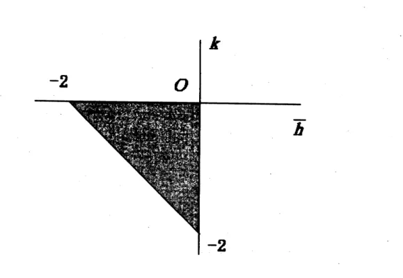
conclude to check the numerical $\mathrm{M}\mathrm{S}$-stability whether the pair $(\overline{h}, k)=$

$(\lambda h, \alpha^{2}/\lambda)$ satisfying $|R(\overline{h}, k)|<1$ for every $\lambda_{1}$ and $\lambda_{2}$

.

Namely we should check $(\overline{h}_{1}, k_{1})=$

$(\lambda_{1}h, \alpha^{2}/\lambda_{1}),$ $(\overline{h}_{2}, k_{2})=(\lambda_{2}h, \alpha^{2}/\lambda_{2})\in \mathcal{R}_{\mathrm{E}\mathrm{M}}$

.

Here $\mathcal{R}_{\mathrm{E}\mathrm{M}}$ is the $\mathrm{M}\mathrm{S}$-stability region of the

Euler-Maruyama scheme in scalar

case.

We will show the region in Fig. 1.

will focus

on

Type $\mathrm{I}\mathrm{I}$

.

We will calculate the $\overline{\mathcal{M}}$ and stability condition

as same

as

Type I.

(6)

Theorem 5Type $II$has the stability $mat\dot{m}$ given by $\overline{\mathcal{M}}=\{$ $r^{2}(\lambda_{1}h)$ $\beta^{2}h$ 0 $\beta^{2}h$ $r^{2}(\lambda_{2}h)$ 0

00

$r(\lambda_{1}h)r(\lambda_{2}h)+\beta^{2}h$ ’ (12)

which brings the stability condition w.r.t.

_||.

$||_{\infty}$ and

||.

$||_{1}$

as

$\max\{(1+\lambda_{1}h)^{2}+|\beta^{2}h|, (1+\lambda_{2}h)^{2}+|\beta^{2}h|\}<1$

.

We result in stabilty function ofthe Euler-Maruyamascheme (scalar case), namely $R(\overline{h}, k)$

again applicable by $\overline{h}=\lambda h,$ _{$k=\beta^{2}/\lambda$} like

as

Type I.

Finaly

we

try to analyze Type III.

Theorem 6For $\Phi eIII$

we

have

$\overline{\mathcal{M}}=[r^{2}(\lambda_{1}\beta^{2}hh)+\alpha^{2}h\alpha\beta hr^{2}(\lambda_{2}h)+\alpha^{2}h\alpha\beta h\beta^{2}hr(\lambda_{1}h)r(\lambda_{2}h)+(\alpha^{2}+\beta^{2})h2\alpha\beta h2\alpha\beta h]$ ,

which irnplies the stability condition $w.r.t$

.

$||\cdot||_{\infty}$

as

$\max\{(1+\lambda_{1}h)^{2}+(|\alpha|+|\beta|)^{2}h, (1+\lambda_{2}h)^{2}+(|\alpha|+|\beta|)^{2}h\}<1$.

Like

as

Type Iand II,

we

conclude that stabilityfunction of the Euler-Maruyama scheme

(scalar case) $R(\overline{h},$k) again applicable with $\overline{h}=\lambda h,$ k _{$=(|\alpha|+|\beta|)^{2}/\lambda$}

.

4Numerical

experiments

In this section

we

will show the confirmation for

our

$\mathrm{M}\mathrm{S}$-stabilty of the Euler-Maruyama

scheme through numerical experiments. We will describe four examples corresponding to

Type $\mathrm{I},$ $\mathrm{I}\mathrm{I}$, and III (2 examples)

as

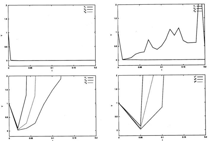
folows. Example 2(Type I)

$\mathrm{d}X=\{\begin{array}{ll}-200 00 -100\end{array}\}X\mathrm{d}t+\{\begin{array}{ll}10 00 \mathrm{l}0\end{array}\}X\mathrm{d}W(t)$ (13)

$h=0.005$, $(\overline{h}, k)=(-1, -0.5),$ $(-0.5, -1)$ : stable

$h=0.01,$ $(\overline{h}, k)=(-2, -0.5),$ $(-1, -1)$ : unstable

$h=0.02,$ $(\overline{h}, k)=(-4, -0.5),$ $(-2, -1)$ : unstable

$h=0.05,$ $(\overline{h}, k)=(-10, -0.5),$$(-5, -1)$ : unstable

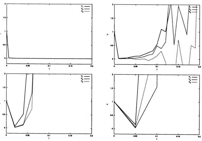
Example 3 $(\infty pe$ II)

$\mathrm{d}X=\{\begin{array}{ll}-200 00 -1\mathrm{O}\mathrm{O}\end{array}\}X\mathrm{d}t+\{\begin{array}{ll}0 1010 0\end{array}\}X\mathrm{d}W(t)$

$h=0.005$, $(\overline{h}, k)=(-1, -0.5),$$(-0.5, -1)$ : stable $h=0.01,$ $(\overline{h}, k)=(-2, -0.5),$$(-1, -1)$ : unstable $h=0.02,$ $(\overline{h}, k)=(-4, -0.5),$ $(-2, -1)$ : unstable $h=0.05,$ $(\overline{h}, k)=(-10, -0.5),$$(-5, -1)$ : unstable

94

(7)

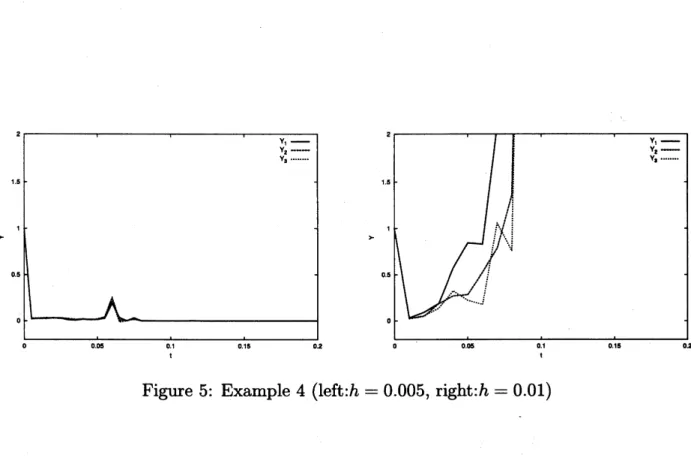
Example 4(Type III)

$\mathrm{d}X=\{\begin{array}{ll}-200 00 -100\end{array}\}X\mathrm{d}t+\{\begin{array}{ll}10 55 10\end{array}\}X\mathrm{d}W(t)$

$h=0.005$, $(\overline{h}, k)=(-1,$$-0.625)$,(-0.5, -1.25) : stable

$h=0.\mathrm{O}1,$ $(\overline{h}, k)=(-2$,-0.625$)$,$(-1,$ $-1.25)$ : unstable

Example 5(Type III)

$\mathrm{d}X=\{\begin{array}{ll}-200 00 -100\end{array}\}X\mathrm{d}t+\{\begin{array}{ll}5 1010 5\end{array}\}X\mathrm{d}W(t)$

$h=0.005$, $(\overline{h}, k)=(-1,$$-0.625)$, (-0.5, -1.25) : stable

$h=0.\mathrm{O}1,$ $(\overline{h}, k)=(-2,$$-0.625)$,$(-1,$ $-1.25)$ : unstable

We took the initial value $X(0)=(1,$ 1) and 10,000 samples. We will show the results of

Example 2to Fig. 2, Example 3to Fig. 3, Example 4to Fig. 4and Example 5to Fig. 5.

5Conclusions and Future

aspects

We extended numerical $\mathrm{M}\mathrm{S}$-stabilityfor ascalar SDE with one multiplicative noise to it for

a2-dimensional SDE system with

one

multiplicative noise. We will analyze $\mathrm{M}\mathrm{S}$-stability for

general pair ofthe matrices $D$ and $B$, and

more

dimensional

case.

And

we

will investigate

the relation of the $\mathrm{M}\mathrm{S}$-stability conditions in matrix norms, for example, between $||\cdot||_{\infty}$ and

$||\cdot||_{2}$

.

Acknowledgement

$\mathrm{s}$

This work is supported by the Grant-in-Aidfor Scientific Research (A) ofJapan Society

for Promotion ofScience (JSPS) (No. 11304004).

References

[1] K. DEKKER and J. G. VERWER, Stability

_of

Runge-Kutta methods

_{for stiff}

nonlinear

differential

equations, North-Holland, Amsterdam,

1984.

[2] T. C. GARD, Introduction to Stochastic

_Differential

Equations, Marcel Dekker, New

York, 1988.

[3] P. E. KLOEDEN and E. PLATEN, The Numerical Solution

_of

Stochastic

_Differential

Equations, Springer, Berlin, 1992.

[4] Y. KOMORI and T. MITSUI, Stable ROW-type weak scheme for stochastic differential

equations, Monte Carlo Methods and Applic., 1(1995), 279-300.

(8)

).] _{Y. KOMORI, Y.}

_sAITO

_{and T.} _MITSUI, _{Some issues} _in $d_{i}screte$ approimate solutior

for

stochastic

_differential

equations, _{Computers Math. Applc.,} _28(1994), _pp.

_269-278.

$)]\backslash$ J. D. LAMBERT, Numerical Methods

for

Orvlinary

_Differential

_{Systems, Wiley,} _New

York,

1991.

7] Y.

SAITO

and T. MITSUI, Stability analysis

_of

numericalschemes

_for

stochcnstic

_differ

$\cdot$

ential equations, SIAM J. Numer. Anal., 33(1996), pp.

2254-2267.

Figure 1: $\mathrm{M}\mathrm{S}$-stability region of

Euler-Maruyama scheme

(9)

$1\mathrm{S}$ $\succ$ $\succ$ $\mathrm{Y},-\mathrm{Y},-\mathrm{Y}^{2}\cdots\cdots\cdot$ .

.

$\mathrm{o}s$ 0 ooe $01|$ $0\prime 5$ $\mathrm{o}z$

Figure 2: Example 1(upper left:h $=0.005$, upper right:h $=0.\mathrm{O}\mathrm{l}$, lower left:h $=0.02$, lower

right:h $=0.05)$

(10)

$\prime s$ $\succ$ $\triangleright$ $\mathrm{Y}..-..\sim\acute{\mathrm{v}}_{*-}^{\prime-}$ . $0\mathrm{S}$ 0 0 $0\alpha$ $\alpha_{1}$ ’ $\propto\prime 5$ 02 $\succ$ $\succ$

Figure

3:

Example 2(upper left:h $=0.005$, upper right:h $=0.\mathrm{O}\mathrm{l}$, lower left:h $=0.02$, lower

right:h $=0.05)$

$\succ$

Figure 4: Example 3 (left:h$=0.005,$right:h $=0.\mathrm{O}\mathrm{l})$

(11)

2 $1B$ $\mathrm{Y}_{s}-\mathrm{Y}_{\acute{2}}---\mathrm{Y}-$ $\mathrm{o}s$ 0 0 ooe $0_{1}1$ 015 $\mathrm{o}s$

Figure 5: Example 4 (left:h $=0.005,$right:h $=0.\mathrm{O}\mathrm{l})$