1.Introduction
This research note describes a novel, hybrid, agent-based and system dynamics (AB-SD) model for an ecological economic system.
Ecological economic systems are undeniably complex (Limburg et al. 2002), and understanding these systems and their behavior is difficult. Models that present a simplified version of the system for the task at hand are therefore required. The question is not whether a model should be used; rather, it is which model to use (Richardson, 2013).
By simplification, a model reveals certain aspects of a system, but not every aspect. Each modeling approach has its own strengths and weaknesses; therefore, the selected modeling approach stipulates which aspects of the system are captured. The complexity of an ecological economic system is also does not respect the strengths and weaknesses of modeling approaches, so we need to tailor modeling approaches to fit the system and the task at hand.
Hybrid models that integrate multiple modeling approaches are becoming a more common approach for complex systems (Swinerd and McNaught, 2012) to meet requirements. Through successful integration, we can take advantage of the strengths of multiple modeling approaches that complement each other to diminish their weaknesses.
This study developed a hybrid AB-SD model for an ecological economic system. The model extends a series of bioeconomic models developed by Clark (2006). A hypothetical ecological economic system is introduced for developing the model. The ecosystem contains fish (as predator) and plankton (as prey), and the economic system is a fish market, forming the fish prices. Fishermen connect the ecosystem to the economic system. The two systems require different levels of abstraction or simplification. The ecosystem is modeled using an agent-based (AB) method, This study developed a novel hybrid agent-based and system dynamics (AB-SD) model for an ecological economic system. The complex nature of an ecological economic system prevents us from seeing the system and its behavior as it is, which calls for a model. A model simplifies reality and reveals certain aspects of it. The modeling approach chosen, however, stipulates what we see, which may not necessarily be what is required for the task at hand. Recent discussions on modeling complex systems propose the integration of multiple modeling approaches. This research note demonstrates that integrating AB and SD could have strong potential for modeling ecological economic systems. In addition to documenting the model, its potential policy implications and issues that guide future research directions are discussed. Keywords: Agent-based modeling; System dynamics; Hybrid modeling; Ecological economic systems; Fishery
which is suitable for modeling individuals (fish, plankton, and fishermen) and spatial heterogeneity. The economic system is modeled using a system dynamics (SD) method, which is suitable for modeling aggregate dynamics (the quantity of fish supplied and demanded). Previous studies on market behavior in AB, which reflect heterogeneous suppliers and consumers, show that prices differ from those in a perfectly competitive market, with homogeneous (or aggregate) producers and consumers (e.g., Epstein and Axtell, 1996). As fish can be considered commodities that are not differentiable for consumers, and a single price could be formed, as explained by textbook microeconomics (Varian, 1992), an aggregate model is suitable for this study.
Four primary objectives of this note study include documenting the hybrid AB-SD model, demonstrating the model’s behavior, and discussing policy implications and issues that could guide future research. While the potential of hybrid AB-S modeling has already been mentioned (Vincenot et al., 2011; Swinerd and McNaught, 2012; Wallentin and Neuwirth, 2017), conducting AB-SD modeling in general is lacking; its application on ecological economic systems is no exception. Further research is suggested “to better understand where and when these classes of hybrid model design are most appropriately applied and to what benefit” (Swinerd and McNaught, 2012, p.119). Swinerd and McNaught (2012) call for its application on the nature of cross-scale systems that may involve different levels of abstraction, as very little work on this has been reported.
2.Material and methods
2.1.Hybrid agent-based and system dynamics modeling
The AB and SD models are both computational approaches to modeling complex systems; however, with disparate approaches towards complexity, they could complement each other (Wallentin and Neuwirth, 2017).
AB is a bottom-up approach “to create, analyze, and experiment with models composed of agents that interact within an environment” (Gilbert, 2008, p.2), and captures the heterogeneity of agents and their environment. Agents interact with each other and their environment, which could create an emergent behavior that cannot be explained without modeling interactions. AB also can determine the spatial dimension of complex systems. SD is a top-down approach that uses aggregate variables, such as population, by assuming that the agents are homogenous (e.g., Uehara, 2013; Uehara et al., 2015). SD is more efficient when heterogeneity and its consequences are not the focal point of the research. While there are some spatial system dynamics models (e.g., Bendor and Kaza, 2012; Cordier et al., 2017), SD is not technically suitable for a spatial modeling.
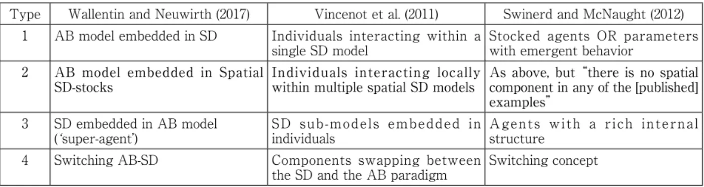
There are various possibilities for integrating AB and SD; these can be classified into four types (Table 1). The type chosen depends on the nature of the system to model and the purpose of the model.
Table 1. Adopted and modified from Wallentin and Neuwirth (2017)
Type Wallentin and Neuwirth (2017) Vincenot et al. (2011) Swinerd and McNaught (2012) 1 AB model embedded in SD Individuals interacting within a
single SD model Stocked agents OR parameters with emergent behavior 2 AB model embedded in Spatial
SD-stocks Individuals interacting locally within multiple spatial SD models As above, but “there is no spatial component in any of the [published] examples”
3 SD embedded in AB model
(‘super-agent’) SD sub-models embedded in individuals Agents with a rich internal structure
4 Switching AB-SD Components swapping between
2.2.The hypothetical case
The primary purpose of this study was to develop an ecological economic model that uses the strengths of SD and AB, rather than deriving policy implications for a specific case, so the situation is purely hypothetical and not based on a real case. Figure 1 shows the overall structure of the model that will be developed.
The ecosystem has fish as the predator and plankton as the prey, and their spatial locations are noted. The economic system is a fish market where fish prices are formed. Fishermen connect the ecosystem to the economic system by catching fish and selling them in the fish market. Fishermen decide how much effort to put into fishing based on revenue from fish sales. In Figure 1, R1 depicts this reinforcing loop to include this decision; a higher fish price raises revenue, which leads to more fishing effort from fishermen, resulting in higher catch and supplied. This is constrained by other balancing loops. For instance, B2 shows that higher supplied dampens fish-price following the law of supply, resulting in lower revenue.
Figure 1. Causal loop diagram of the ecological economic model. R and B indicate reinforcing loop and balancing loop, respectively.
AB SD
The ecological dynamics of fish and plankton, along with fishermen catching fish, are better modeled by AB because of their spatial heterogeneity. The fish market, however, is better modeled by SD, because fish is a commodity and consumers cannot differentiate one fish from another, i.e., fish are homogenous in the market. Additionally, fishermen bring the fish to the market, and they are a price taker in a perfectly competitive market. Therefore, computing fish prices using an aggregation of fish demanded and supplied is suitable.
3.The model
The model extends a series of bioeconomic models developed by Clark (2006). The major extensions are 1) reflecting heterogeneities regarding fishermen, fish, and plankton, and 2) enabling the adjustment of fish prices in the fish market to account for demand and supply. NetLogo (Version 6.0.1) by Uri Wilensky (https://ccl.northwestern. edu/netlogo/), a piece of software primarily designed for AB modeling, was used. The software is also capable of system dynamics modeling. The code for the model is in the Appendices, and the NetLogo model can be provided upon request.
3.1.Fisherman’s behavior
The fisherman’s behavior is modeled by AB to reflect the heterogeneity of fishermen and their environment (e.g., the amount of fish they can catch).
Following Clark (2006), revenue R is given by the difference between sales and costs, as shown in Eq. 1. The time notation is suppressed when it is not necessary.
(1) where p, Y(E, S), and C(E) are fish price, yield (catch), and costs, respectively. Yield is a function of fishing effort E and fish biomass S. Costs are a function of E. Clark (2006) proposes a simple specification:
(2) where q is catchability, and the cost is assumed to be proportional to effort and not fixed.
qSE is called the Schaefer catch equation (Clark, 2006) and assumes that catch is proportional to biomass S, therefore catch per unit effort Y(E, S)/E=qS will decrease when the abundance of the biomass S decreases from greater catch. However, as Clark (2006) claims, the equation “should be considered the exception rather than the rule in fish biology” (Clark, 2006, p.43). The equation is valid if “the fish population responds to reduction in numbers by redistributing itself uniformly over the whole fishing area.” (Clark, 2006, p.43).
The model presented here overcomes this problem by utilizing the strengths of AB. While S influences the amount of the fish that a fisherman meets in his location, it is not appropriate to use it as if its impact is distributed uniformly over the whole fishing area. Therefore, S is replaced with si, the amount of fish a fisherman i (i=1, ...n) meets in the area where the fisherman is located. While si, l (l=1, ..., L) is influenced by S (depending on how many fish swim across the area), it does not mean that S impacts si, l uniformly across location l. si, l is computed by AB.
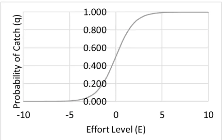
qE is replaced with q(E), which has properties of q'(E)>0, q''(E)<0, q(0)=0, limE →∞q(E)=1. The following sigmoid function is adopted to show these properties.
Figure 2. The behavior of the sigmoid function
(3) and
(4) The function behaves as shown in figure 2.
Each fisherman may receive different profit, and the revenue function is given by
(5) The parameters with subscript i could take a unique value for each fisherman; every fisherman faces the same fish price p, which is determined in the market simulated in SD (Eq. 11).
A fisherman makes a decision on his effort level to maximize his revenue R:
(6) The first-order condition is
(7) This provides a solution where a fisherman can optimize Ri instantaneously. However, since Si,l depends on the location of the fisherman (i.e., l) and p is determined by the market, which is beyond the fisherman’s control, choosing Ei (which satisfies the first-order condition that assumes that Si,l and p are constant) may not necessarily lead to maximum revenue. Therefore, it may be more reasonable to assume that the fisherman gradually changes his effort level.
(8)
Adjustment Timei determines how fast the fisherman updates his effort level. Longer adjustment times mean that it takes more time for him to change his effort level. Adjustment Timei = 1 means that the effort level is updated instantaneously to make Et at the level where revenue is maximized if the fisherman faces the same situation as the previous period t - 1.
Y(Ei, st,l) depends on st,l, which is beyond the fisherman’s control. st,l and Y(Ei, st,l) are heterogeneous, as explained below. A fisherman’s behavior is modeled in AB (see Appendices for technical details). A fisherman moves one step in a randomly chosen direction at each time period. “One step” in AB means “to move to an adjacent patch” ; hence whether he moves to a patch with high st,l or not is luck.
3.2.Ecosystem dynamics
The ecosystem dynamics are modeled in AB. The ecosystem comprises one agent type fish (predator) and one patch type, plankton (prey). While the fish move across the area, plankton stay in the same location. If we ignore the heterogeneity of fish and plankton, ecosystem dynamics, i.e., the dynamics of fish, , and plankton, , can be expressed by the two sets of differential equations as follows:
(9) (10) where G(S, X) is the net reproduction rate of the fish biomass S, g(X) is the net reproduction rate of plankton X, and h(S) is the plankton harvest by the fish.
While equations (9) and (10) capture the overall behavior of the model, each fish and plankton behave heterogeneously, following the rules below (see Appendix for details).
For each time period, a fish moves to an adjacent patch in a randomly chosen direction, consuming energy to swim. If there is enough plankton, the fish can increase its energy. The fish gives birth if its energy is above a certain threshold, and dies when it has no remaining energy.
Plankton do not move, but stay in a patch. Their abundance decreases when the fish eat them and increases when they reproduce.
3.3.Fish market
The fish market is where fish prices are formed based on the quantities of fish supplied and demanded. Textbook microeconomic theory assumes an instantaneous equilibrium; however, it is assumed that price changes gradually. This assumption should be reasonable when supply and/or demand is as volatile as a fish market where fish catch fluctuates significantly, including no catch.
To model this adjustment process, the hill-climbing method was adopted (Sterman, 2000). The hill-climbing method is a technique for adjusting the state of a system (i.e., fish price) until it reaches the desired state (i.e., market clearing or equilibrium fish price), as shown in Figure 3.
Figure 3. Stock and flow diagram of the SD module
The SD module in Figure 3 can be addressed with a system of equations as follows.
(11) (12) (13) As there is a possibility of no quantity of supplied (i.e., zero catch), the if else function is used, as follows:
(14)
(15)
while is computed by SD, is computed by AB.
The demand curve is a simple linear function of fish price, with a choke price where the demand reaches zero if the price is too high.
(16)
4.Simulation results
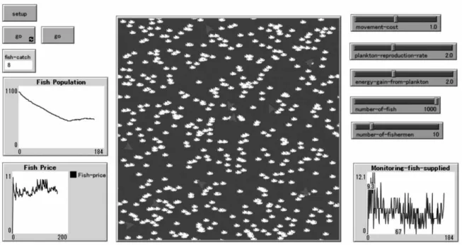
This section reports the key behaviors of the model. As the primary purpose of this study was to develop a novel hybrid AB-SD model for an ecological economic system, the parameters chosen are not firmly based on empirical data (see Appendices for parameter values). Figure 4 shows a screenshot of the interface of the AB.
Figure 4. Screenshot of the AB interface
When the fishermen catch no fish, fish population increases but is bounded at some point due to limited plankton availability (Figure 5). When the fishermen catch fish, the fish population decreases but is stabilized at some point (Figure 6); fish catch (Figure 7) is a mirror image of these dynamics. The stabilization could be due fish prices, which are formed through interactions between demand and supply. Two balancing feedback loops regulate fish demanded and supplied supply (Figure 1). Fish prices are stabilized around the equilibrium prices because of this price mechanism, along with the fixed demand curve (Figure 8).
Figure 5. Fish population without fish catch
Figure 7. Fish catch with fish catch.
The black line is a trend line with moving average = 10.
Figure 6. Fish population with fish catch
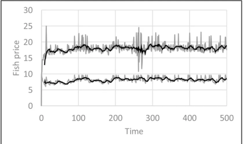
Figure 8. Fish price with fish catch.
Figure 9. Fish price with fish catch with a higher intercept. The black line is a trend line with moving average = 10.
To further study the model’s behavior, the impacts of changes to fish demand on fish prices were simulated.
Figure 9 and Table 2 compare two cases: the baseline demand curve ( ), and a
demand curve with a higher intercept ( ). While higher overall prices were
expected, higher volatility (e.g., larger extreme values and higher standard deviation) requires further investigation to understand the logic behind the dynamics.
5.Conclusion and future research directions
This research note documented a novel, hybrid AB-SD model for an ecological economic system. Ecological economic systems are complex; one of the attributes of their complexity is that they require different levels of abstraction, which in turn requires hybrid modeling that integrates multiple approaches. While AB is suitable for disaggregation, SD is suitable for aggregation. Integrating AB and SD models meets this requirement. In the hybrid model, AB captures disaggregated ecosystem dynamics, consisting of fish and plankton, and SD captures the dynamics of the fish market in an aggregate manner. Fishermen, whose behaviors are modeled in both AB and SD, connect the ecosystem to the economic system.
There are several caveats and future research questions. Owing to the complexity of an ecological economic model and its behavior, model tests are essential before deriving any policy implications, otherwise the implications would be unreliable. There are various testing methods available for both AB and SD (e.g., Sterman, 2000; Railsback and Grimm, 2011). The hybrid model uses two distinct modeling approaches, which could pose further challenges to model tests; therefore, the development of model testing methods for hybrid modeling could be an important direction for future research.
The model can be extended further. For example, we could develop more realistic policy implications using real spatial data from geographic information systems (GIS). AB is compatible with GIS (Wallentin, 2017); Lindholm et al. (2001) tested the effectiveness of marine protected areas by studying spatial variations in seafloor habitat.
Table 2. Comparison of mean values and standard deviations
Demand function Mean Standard Deviation 8.054758167 0.818363929 17.91946214 1.79490971
As hybrid AB-SD modeling is an emerging, and yet mature, field, software choice matters. Although NetLogo software was used in this study, there are other choices available (e.g., Ventity (http://ventity.biz/) and AnyLogic (https://www.anylogic.com/)) and each piece of software has different strengths and weaknesses. The choice of software should be made based on the purpose of the modeling.
Appendices
Appendix A. Code for the AB component
breed [fish a-fish]
breed [fishermen fisherman]
fish-own [ energy ] ;; fish own energy
fishermen-own [ fish-catch target fishing-effort]
patches-own [ plankton-amount ] ;; patches have plankton ;; this procedures sets up the model
to setup clear-all ask patches [ set pcolor blue
random-seed 1234 ;; set the random-seed to generate the same result (note that it might be different when the model is run on a different version)
set plankton-amount random-float 10.0 ]
create-fish number-of-fish [ ;; create the initial fish setxy random-xcor random-ycor
set color white set shape "fish"
set energy random 100 ;; if we want to set energy range 0 to 100 uniform distribution, random 100 ]
create-fishermen number-of-fishermen [ ;; create the initial fishermen setxy random-xcor random-ycor
set color red set shape "default"
set size 2 ;; increase their size so they are a little easier to see set fishing-effort 0.5 ;; everyone starts with the same fishing effort ] system-dynamics-setup system-dynamics-do-plot reset-ticks end to go ask fish [
check-if-dead ;; checks to see if fish should die wiggle ;; first turn a little bit in each direction
reproduce-plankton ;; the plankton reproduce back system-dynamics-go
system-dynamics-do-plot tick
end
;; fish procedure, ask those fish with no energy to die to check-if-dead
if energy < 0 [ die
] end
;; fish and fishermen procedure, the fish changes its heading to wiggle
;; turn right then left, so the average is straight ahead right random 90
left random 90 end
;; fish and fishermen procedure to move
forward 1 ;; take a step forward
set energy energy - movement-cost ;; reduce the energy by the cost of movement end
;; fishermen procedure to search
forward 1 ;; take a step forward end
;; fish procedure, fish eat plankton to eat
;; check to make sure there is plankton here
if ( plankton-amount >= energy-gain-from-plankton ) [ ;; increment the fish's energy
set energy energy + energy-gain-from-plankton ;; decrement the plankton
set plankton-amount plankton-amount - energy-gain-from-plankton ] end ;; fish procedure to reproduce if energy > 200 [
set energy energy - 100 ;; reproduction transfers energy hatch 1 [ set energy 100 ] ;; to the new fish
] end
;; reproduce the plankton to reproduce-plankton ask patches [
set plankton-amount plankton-amount + plankton-reproduction-rate if plankton-amount > 10.0 [ set plankton-amount 10.0 ] ] end to clear-stats
ask fishermen [ set fish-catch 0] end
to catch
if any? fish-here [ ;; if there are fish here then catch them set target fish-here
set fish-catch count target ask target [ die ] ] show fish-catch end to effort-decision
let MR Fish-price * fish-catch * (exp (-1 * fishing-effort)) / (1 + exp (-1 * fishing-effort)) let MC 10 * 2 * fishing-effort ;; MC=2E
set fishing-effort (1 + 0.1 * ((MR - MC) / MC)) * fishing-effort ;; adjustment time 1/10 ;;show fishing-effort
;;show MR end
;; Copyright 2017 Takuro Uehara ;; [email protected] ;; Ritsumeikan University
;; Initializes the system dynamics model. ;; Call this in your model's SETUP procedure. to system-dynamics-setup
reset-ticks set dt 1.0
;; initialize constant values set Price-adjustment-time 10 ;; initialize stock values set Fish-price 10 end
;; Step through the system dynamics model by performing next iteration of Euler's method. ;; Call this in your model's GO procedure.
to system-dynamics-go
;; compute variable and flow values once per step let local-Fish-supplied Fish-supplied
let local-Fish-demanded Fish-demanded
let local-Effect-of-demand/supply-balance-on-fish-price Effect-of-demand/supply-balance-on-fish-price let local-Indicated-fish-price Indicated-fish-price
let local-Change-in-price Change-in-price ;; update stock values
;; use temporary variables so order of computation doesn't affect result. let new-Fish-price ( Fish-price + local-Change-in-price )
set Fish-price new-Fish-price tick-advance dt
end
;; Report value of flow to-report Change-in-price
report ( (1 / Price-adjustment-time) * (Indicated-fish-price - Fish-price) ) * dt
end
to-report Fish-supplied
report sum [fish-catch] of fishermen end
;; Report value of variable to-report Fish-demanded
report 15 + (15 / (5 - 15 )) * Fish-price
;; it goes through (Qd, P) = (5,1) and (15, 0). Numbers are chosen so as to stabilize the results. end
;; Report value of variable
to-report Effect-of-demand/supply-balance-on-fish-price report ifelse-value (Fish-supplied = 0)
[1]
[Fish-demanded / Fish-supplied]
;; When there is no catch, the market does not open (i.e., the price does not change). end
;; Report value of variable to-report Indicated-fish-price
report Effect-of-demand/supply-balance-on-fish-price * Fish-price end
;; Plot the current state of the system dynamics model's stocks ;; Call this procedure in your plot's update commands.
to system-dynamics-do-plot if plot-pen-exists? "Fish-price" [ set-current-plot-pen "Fish-price" plotxy ticks Fish-price
] End
system dynamics model and cellular automata model. Science in China Series D: Earth Sciences 48, 1979-1989. Limburg, K.E., O'Neill, R.V., Costanza, R., Farber, S., 2002. Complex systems and valuation. Ecological Economics 41, 409-420. Lindholm, J.B., Auster, P.J., Ruth, M., Kaufman, L., 2001. Modeling the Effects of Fishing and Implications for the Design of Marine
Protected Areas: Juvenile Fish Responses to Variations in Seafloor Habitat.
Railsback, S. F., & Grimm, V. 2011. Agent-based and individual-based modeling: a practical introduction. Princeton university press. Richardson, J. 2013. The past is prologue: reflections on forty ‐ plus years of system dynamics modeling practice. System Dynamics
Review, 29(3), 172-187.
Sterman, J.D., 2000. Business dynamics: systems thinking and modeling for a complex world. Irwin/McGraw-Hill Boston.
Swinerd, C., McNaught, K.R., 2012. Design classes for hybrid simulations involving agent-based and system dynamics models. Simulation Modelling Practice and Theory 25, 118-133.
Uehara, T., 2013. Ecological threshold and ecological economic threshold: Implications from an ecological economic model with adaptation. Ecological Economics 93, 374-384.
Uehara, T., Nagase, Y., & Wakeland, W. 2015. Integrating Economics and System Dynamics Approaches for Modelling an Ecological–Economic System. Systems Research and Behavioral Science, 33(4), 515-531.
Varian, H. R. 1992. Microeconomic Analysis, WW Norton&Company. Inc, New York, New York.
Vincenot, C.E., Giannino, F., Rietkerk, M., Moriya, K., Mazzoleni, S., 2011. Theoretical considerations on the combined use of System Dynamics and individual-based modeling in ecology. Ecological Modelling 222, 210-218.
Wallentin, G., 2017. Spatial simulation: A spatial perspective on individual-based ecology—a review. Ecological Modelling 350, 30-41. Wallentin, G., Neuwirth, C., 2017. Dynamic hybrid modelling: Switching between AB and SD designs of a predator-prey model.