The method of Hill determinants in PT-symmetric quantum mechanics (Recent Trends in Exponential Asymptotics)

The method of Hill determinants in PT-symmetric

quantum

mechanics

Miloslav Znojil

Ustav jaderne fyziky AV

\v{C}R,

25068

\v{R}e\v{z},

Czech Republic

Abstract

Hill-determinant method is described and shown applicable within the

so

called

PT-symmetric quantum mechanics. We demonstrate that in

a

way paralleling its

tradi-tional Hermitian applications and proofsthe methodguarantees thenecessary

asymp-totic decrease of

wave

functions $\psi(x)$

as

resulting from a fine-tuned mutual

cancel-lation of their asymptotically growing exponential components. Technically, the

rig-orous proof is needed/offered that in a quasi-variational spirit the method allows

us

to work, in its numericai implementations, with a sequence oftruncated forms ofthe

rigorous Hill-determinant power series for the normalizablebound states $\psi(x)$.

PACS 03.65.Ge, 03.65.Fd

1

Introduction

One of the key sources of an

enormous

popuiarity of one-dimensional

anharmonic-oscillator Schr\"odinger equations

$(- \frac{d^{2}}{dx^{2}}+V(x))\psi(x)=E\psi(x)$, $x\in(-\infty, \infty)$ (1)

with polynomial potentials, say, of the quartic form

$V(x)=ax^{4}+bx^{3}+cx^{2}+dx$_{, $a=1$ (2)}

lies, definitely, in their_{methodically illuminating role ofapparently “next-to-solvable”}

Thirty five years ago one of the characteristic results in this direction has been

obtained by Benderand Wu [1] who made

a

highly nontrivial observation that in

some

models ofsuch

a

type, all the pertainingbound-state energies $E_{n}$ may be understood

as

valuesofa single analytic function when evaluated on its different Riemann sheets.

This observation (made at $b=d=0$)

was a

real breakthrough in the intensive

con-temporary perturbative analysis ofeq. (1) $+(2)$

.

Later on, it hasbeen complemented

bythe alternative semi-classical [2] and quasi-variational [3] sophisticated treatments

of eq. (2). In this sense, themodelprovided

an

extremely useful insight in the possible

structures encountered within relativistic quantum field theory [4].

The hypotheses of ref. [1] have also been explicitly verified in the

phenomeno-logicaiiy equally important cubic-oscillator limit $aarrow 0$ [5]. In paralJel, the closely

interrelated semi-classicai and quasi-variational (often called Hill-determinant, HD)

constructions of bound states were subsequently generalized to virtually all

polyno-mials $V(x)$. In the former semi-classical setting, an updated sample ofreferences is

offered by these proceedings. In contrast, the parallel HD approach to polynomial

$V(x)[6]$

seems

“forgotten” at present, in spite of its extremely useful capability of

complementing the perturbative and semi-classical constructions. This is

one

of the

reasons

why the forthcoming text has been written for the

same

proceedings.

A nice illustration of the HD-semi-classicalcomplementarity ofthecorresponding

algorithms has been thoroughly described in ref, _{[7] (here,}

_we

_shall skip this

illus-tration referring to the original paper containing

a

few numerical tables and further

references).

The HD methodemphasizescertain important non-perturbative featuresofthe

en-ergies. Again

we

wouldlike to recollect

an

elementaryillustrative two-dimensional

ex-ample ofref. [8],

or a

more

extensive one-dimensional sextic-oscillatorstudy [9] where

the HD-type energies have been specified

as

roots of

a

convergent continued fraction.

Unfortunately, in the contemporary literature at least, the acceptance and credibility

of the HD approach to polynomiai $V(x)$ has been marred, in the quasi-variational

context

as

well

as

in perturbation theory, by a few unfortunate misunderstandings

concerning the related mathematics.

For

a

sketchy explanation ofthe latter point the reader should consult the twenty

years old Hautot’s concise review [10]. A

more

thorough account of the problem

may be found in my

own

long and unpublished dissertation [11] including references

misunderstanding up to these days) as well as

a

detailed account and an exhaustive

specification ofthe domain ofvalidity of the HD techniques in Herm itian

cases

with

polynomial potentials.

The present updated HD review is going to move one step further. The

reason

is

that in the light of

some

most recent semi-classical analyses ofanharmonicoscillators,

another important motivation for

a

renewal of interest in HD philosophy might be

found inthe formal parallels between these two techniques, both having to deaf with

complexified coordinates and both beingbased on the infinite-series expansions of the

energies $E$ and of the related

wave

functions $\psi(x)$, respectively. It is also worth

a

marginal note that in both ofthem a different role is played by certain exponentially

suppressed small contributions.

2

$P\mathcal{T}$

-symmetric

quantum

mechanics

Within the framework ofthe pure quantum physics, the idea of

a

complexification of

the couplings

or

coordinates is in fact neither too popular

nor

formally welcome. A

characteristic comment has been made by the author of [4] whose historical remarks

clarified the situation in the seventies when people im agined that the convergence

ofperturbation series would imply that the “observables” may be well defined

even

when the Hamiltoniansthemselves become manifestly non-Hermitian.

For this reason, perhaps, Carl Bender needed almost thirtyyears

more

to returnto

the complexified models in the two pioneering papers [12] where thetwo

new

versions

ofeq. (2) have been studied with the purely imaginary couplings $b=if:$ and $d=i\mathit{6}.$

The emphasis has been laid upon quite amazing

an

observation that the spectrum

remains real in spite of the obvious fact that $H\neq H^{\uparrow}$

.

In the light of the possible

applications of suchanapproachin Quantum Mechanics, the authorscharacterized the

underlying specific non-Hermiticity as a “weakened Hermiticity”

or

“$P\mathcal{T}$symmetry”

ofthe Hamiltonian. Indeed, in their most elementary models the operators $P$ and $\mathcal{T}$

denoted the parity and the time reversal (i.e., in effect, the Hermitian conjugation),

respectively.

The methods they used

were

mainly perturbative and semi-classical. In what

folJows,

we

intend to

answer

the question whether

some

models of PT-symmetric

quantum mechanics could admit the constructive solution of their Schr\"odinger

employing

our

recent results in [13],

we

shall mainlyreview the results concerning the

above-mentioned quartic problem

$(- \frac{d^{2}}{dx^{2}}+x^{4}+\mathrm{i}\beta x^{3}+cx^{2}+\mathrm{i}\delta x)\psi(x)=E\psi(x)$, $x\in(-\infty, \infty)$ (3)

again, with the real values of $\beta,$ $c$ and $\delta$ and, therefore, with the manifestly

non-Hermitian, $P\mathcal{T}$-symmetric form of the Hamiltonian.

Before getting in

more

details, let

us

only add that during the rapid development

of the field (summarized, e.g., in the proceedings ofthe recent Workshop which have

to appear in the October issue of Czechoslovak Journal of Physics this year), the

“parity” $P$ should be understood, in a broader sense,

as

an

arbitrary (Hermitian and

invertible) operator of a pseudo-metric $\eta(pseud\mathrm{o})$ in Hilbert space [14]. Similarly, the

symbol $\mathcal{T}$ should be understood

as an

antilinear operator mediating the Hermitian

conjugation of$H[15]$.

In the context ofphysical applications, the concept ofthe “parity” itself becomes

insufficient and must be complemented by a “quasi-parity” operator $Q[16]$ which

makes the scalar products (between eigenstates of $H\neq H^{\{}$) positively definite [17].

This

means

that

we

must perform

a

highlynontrivial transitionfrom the non-singular

and, by assumption, indeterminate original pseudo-metric $P=\eta(\mathrm{p}seudo)=\eta_{(\mathrm{p}seudo)}^{\dagger}$ to

some

other, positively definite “true” metric $QP=\eta_{+}>0$, the knowledge of which

allows

us

to call our Hamiltonians $H\neq H^{\{}$ “quasi-Hermitian” and “physical” again

(cf. the reviews [18] for

more

details). In the other words, only the change of the

metric $\prime p\prec QP=\eta(quasi)=\eta_{(quasi)}^{\dagger}$ (where, at present, the

name

“charge” for $Q\equiv \mathrm{C}$

is being preferred [19]$)$ makes the non-Hermitian $P\mathcal{T}$-symmetric models with real

spectrum fully compatible with the probabilistic interpretation and other postulates

ofquantum mechanics in

a

way illustratedvery recently onthe non-Hermitian square

well $[20, 21]$.

3

HD

construction

The

wave

functions $\psi(x)$ definedby eq. (3)

are

analytic at all the complex$x\in C$. In

the asymptotic region ofthe large $|x|\gg 1$ the semi-classical analysis reveals that

$\psi^{(AHO)}(x)\sim\{$

$c_{phys}e^{-x^{3}/3}+c_{vnphys}e^{+x^{3}/3}$, $0\leq|{\rm Im}(x)|\ll+{\rm Re}(x)/\sqrt{3}$,

(4)

The HD method proceeds, traditionally, in an opposite direction and employs the power-series formulae for $\psi(x)$ near the origin. Thus, in the $P\mathcal{T}$-symmetric

manner

we write

$\psi^{\langle ansatz)}(x)=e^{-sx^{2}}\sum_{n=0}^{\infty}h_{n}(\mathrm{i}x)^{n}$ , $x\in(-\infty, \infty)$ (5)

with a suitable (optional) value of $s$. The key

reason

may be seen in the

success

of such

a

strategy in the harmonic-oscillator

case

where such an ansatz converts the

differential Schr\"odinger equation (3) into solvable

recurrences.

Here, of course, the

resulting recurrent rule

$A_{n}h_{n+2}+C_{n}h_{n}+\delta h_{n-1}+\theta h_{n-2}-\beta h_{n-3}+h_{n-4}=0$ (6)

$A_{n}=(n+1)(n+2)$, $C_{n}=4sn+2s-E_{1}$ $\theta=4s^{2}-c$

isnot solvable in closed form. At $\mathrm{a}\mathrm{I}1$theparameters (includingalso theunconstrained,

variable energy $E$), it only defines the coefficients $h_{n}$

as

superpositions

$h_{n}=h_{0}\sigma_{n}+h_{1}\omega_{n}$, $\sigma_{0}=\omega_{1}=1$, $\sigma_{1}=\omega_{0}=0$ (7)

where all thethree sequences $h_{n},$ $\sigma_{n}$ and $\omega_{n}$satisfy the

same

recurrences

withdifferent

initial conditions. Still, we may write the latter two funtions of$n$ in

a

very compact

determinantal form

$\sigma_{n+1}=(-1)^{n}\frac{\det\Sigma_{n-1}}{n!(n+1)!}$ , $\omega_{n+1}=(-1)^{n}\frac{\det\Omega_{n-1}}{n!(n+1)’!}$ , $n=1,2,$ $\ldots$

with $(m+1)$_{-dimensional matrices}

$\Sigma_{m}=$ $\backslash /C_{0}0\mathit{6}1.\cdot.\cdot.\cdot$

$-\cdot..\beta C_{2}A_{0}01^{\cdot}.\cdot C_{3}A_{1}0..\cdot.\cdot$

. $\cdot.A_{2}\delta.\cdot.\cdot$ $C_{\dot{m}_{\mathit{6}}-1}0^{\cdot}$

.

$A_{m_{0}-2}C_{m}$ $A_{m_{0}-1}\ovalbox{\tt\small REJECT}$ (8)

(note: the second column ofthe matrix of the linear system (6) is omitted here since

$\sigma_{1}=0)$ and

$\Omega_{m}=\ovalbox{\tt\small REJECT} C_{1}0\delta 1^{\cdot}.$. $.A_{0}c_{2}^{0}\mathit{6}.\cdot.\cdot$ . $A_{1}C_{\mathrm{S}}0\mathit{6}1^{\cdot}.$ . $\cdot.A_{2}\circ\cdot..\cdot.$

.

$C_{m_{\mathit{6}}-1}0^{\cdot}$ . $A_{m-2}c_{m}^{0}$ $A_{m_{\mathrm{O}}-1}\ovalbox{\tt\small REJECT}$ (9)

(now the first column is omitted in the light of

our

choice of$\omega_{0}=0$).

It remains for

us

to specify the

norm

$\rho=\sqrt{h_{0}^{2}+h_{1}^{2}}l$, the ratio $h_{1}/h_{0}\equiv\tan\zeta$ and

the physical energy $E$ which entersthe $(m+1)$-dimensional matrices (8) and (9). In

the other words,

our

wave

functions $\psi(x)$ must be made “physical” via the standard

boundary conditions

$\psi^{(ansatz)}(X_{R})=0=\psi^{(ansatz)}(-X_{L}))$ $X_{R}>>1_{\mathrm{J}}$ $X_{L}\gg 1$

.

(10)

These conditions play, obviously, the role of

an

implicit definition of the above free

parameters. Nevertheless,

our

ambitions

are

higher and in the HD approach people

usually try to replace eq. (10) by a quasi-variational finite-matrix truncation of eq.

(6) [10], i.e., equivalently, by innovated difference-equation boundary conditions

$h_{N}=h_{N+1}=0$, $N>>1$, (11)

with

a

much simpler numerical implementation. Of course, such

a

replacement ofeq.

(10) by eq. (11) is not always wellfounded [10]

so

that in each particular

construction

its validity must be based on

a

rigorous

mathematical

proof, in a way illustrated in

what follows.

4

The

proof

4.1

The

s

-dependence

of the

asymptotics

of

$h_{n}$

In the first step ofthe proof, the

recurrences

(6) should be read

as

a

linear difference

$h_{n}$ may be found by the standard techniques. Thus, the leading-order solution may

be extracted from eq. (6) by its reduction to its two-term dominant form of relation

between $h_{n+2}$ and $h_{n-4}$. Thus, we put

$h_{n}(p)= \frac{\lambda^{n}(p)g_{n}(p)}{(3^{1/3})^{n}\Gamma(1+n/3)}$ $(12_{J}^{\backslash }$

where the integer $p=1,2,$ $\ldots,$$6$ numbers the six independent solutions and where

$\lambda(p)=\exp[\mathrm{i}(2p-1)\pi/6]$. The

new

coefficients $g_{n}=g_{n}(p)$ vary

more

slowly with

$n$. Thus,

our

first conclusion is that at the large indices $n$, all solutions decrease

as

$h_{n}\sim \mathcal{O}(n^{-n/3})$ at least. This

means

that in a way confirming

our

expectations the

radius ofconvergence of

our

Taylor series (5) is always infinite.

Onthis level of precision the size ofour six independent solutions remains

asymp-totically the same. In order to

remove

this degeneracy

we

amend equation (6) and

having temporarily dropped the$p’ \mathrm{s}$

we

get

$g_{n+2}-g_{n-4}= \frac{4s\lambda^{4}}{n^{1/3}}g_{n}-\frac{\beta\lambda}{n^{1/3}}g_{n-3}+\mathcal{O}(\frac{g_{n}}{n^{2/3}})$

.

(13)

The smallness of $1/n^{1/3}$ in the asymptotic region of_$n>>1$ enables

us

to infer that

$g_{n}=e^{\gamma n^{2/3}+\mathcal{O}(n^{1/3})}$, _{$\gamma=\gamma(p)=s\lambda^{4}(p)-\beta\lambda(p)/4$}, (14)

$\mathrm{i}.\mathrm{e}.$,

${\rm Re} \gamma(1)={\rm Re}\gamma(6)=-\frac{\sqrt{3}}{8}\beta-\frac{s}{2}$ ,

${\rm Re}\gamma(2)={\rm Re}\gamma(5)=s$,

${\rm Re} \gamma(3)={\rm Re}\gamma(4)=\frac{\sqrt{3}}{8}\beta-\frac{s}{2}$. (15)

We may conclude that whenever

we

satisfy the condition

$s> \frac{|\beta|}{4\sqrt{3}}$ (16)

the general, six-parametric _{form ofthe Taylor coefficients}

$h_{n}= \sum_{p=1}^{6}G_{p}h_{n}(p)$ (17)

will be equivalent to the two-term formula in the leading order,

i.e., only its two dominant components remain asymptotically relevant while, in the

leading order,

we

may simply put $G_{1}=G_{3}=G_{4}=G_{6}=0$ in eq. (17) at $n\gg 1$

.

The

same

argument implies that for

$s< \frac{|\beta|}{4\sqrt{3}}$ (19) we get $h_{n}=\{$ $G_{3}h_{n}(3)+G_{4}h_{n}(4)$, $\beta>0,$ $n\gg 1$, $G_{1}h_{n}(1)+G_{6}h_{n}(6)$, $\beta<0,$ $n>>1$. (20)

while the degeneracy of

more

than two soiutions survives at $\beta=0$

or

at $s= \frac{|\beta|}{4\sqrt{3}}>0$

.

4.2

Single-term

dominant

exponentials

in

$\psi^{(ansatz)}(x)$

We know that the shape of the function $\psi^{(ansatz)}(x)$ is determined by the energy $E$

and by the not yet fully specified choice of the two coefficients $h_{0}$ and $h_{1}$

.

In the

language of the preceding section, each choice ofthe energy $E$ and of the initial $h_{0}$

and $h_{1}$ will generate a different, $x-$ and $n$-independent pair ofthe coefficients $G_{2}$

and $G_{5}$ in $h_{n}$ at thesufficiently large $s$ (thediscussion of the smaller $s$ willbe omitted

for the sake ofbrevity).

As long

as our

aimis acompletionof the proofofthe validity of the replacement of

the standard boundary conditions (10) (containinginfinitesums) by the

more

natural

HD truncation of

recurrences

due to eq. (11),

we

just have to paraliel the

Hermi-tian considerations of ref. [22]. Firstly,

we

remind the reader that at an arbitrary

finite precision

we

always have $E\neq E(phys\mathrm{i}cal)$. This

means

that

our

infinite series

$\psi^{(ansatz)}(x)$

as

defined by equation (5) will always exhibit

an

exponential asymptotic

growth in

a

certain wedge-shaped vicinity of the real line [12].

The main point oftheHD proof is thatdue to thestandard oscillationtheorems the

last (left

as

well

as

right) nodal

zeros

will

move

towards their (left and right) infinities

with the decrease of $E>E(phys\mathrm{i}cal)$ (say, at

a

fixed pair $h_{0,1}$). In the language

of coordinates this

means

that the values of $\psi^{(ansatz)}(x)$ (both at

some

$x>X_{R}$ and

at another $x<X_{L}$) will change sign for $E$ somewhere in between the (smaller)

$E$(physical) and (larger) $E(numer\mathrm{i}cal)$. Such a simultaneous change ofthe sign of

$\psi^{\langle ansatz)}(x)$ at any sufficiently large absolute value ofthe coordinate $|x|\gg 1$ should

Although this sounds like a paradox, this estimate will always lead to an

asymp-totic growth (since $E\neq E_{physical}$ with probability one)

so

that it cannot be changed

by the (key) omission ofany

_finite

number $N$ of the exponentially small components

$\sim\exp[-sx^{2}+\mathcal{O}(\ln x)]$. They may besafety ignored

as

irrelevant. This

means

that

we

may choose $N>>1$

so

that just the asymptoticallydominant coefficients will playthe

role. Inserting (12) and (18) in $\psi^{(ansatz)}(x)$ $\sim\exp(-sx^{2})\Sigma_{n=N+1}^{\infty}h_{n}(\mathrm{i}x)^{n}$

we

finally

get

$\psi^{(ansatz)}(x)\sim e^{-sx^{2}}\sum_{n=N+1}^{\infty}\frac{G_{2}\lambda^{n}(2)g_{n}(2)+G_{5}\lambda^{n}(5)g_{n}(5)}{(3^{1/3})^{n}\Gamma(1+n/3)}(ix)^{n}$ , $|x|>>1$

.

The validity of this formula is a strict consequence of the specific constraint (16)

imposed (say, from

now

on) upon the admissible quasi-variational parameter $s$

.

Once we split $\psi^{(ansatz)}(x)=\psi^{(ansatz)}$($G_{2}$,G5,$x$) in its two components

$\psi^{(ansatz)}(G_{2},0, x)\sim G_{2}e^{-sx^{2}}\sum_{n=N+1}^{\infty}\frac{(-x)^{n}\exp[\gamma(2)n^{2/3}+\mathcal{O}(n^{1/3})]}{(3^{1/3})^{n}\Gamma(1+n/3)}$,

$\psi^{(ansatz)}(0, G_{5}, x)\sim G_{5}e^{-sx^{2}}\sum_{n=N+1}^{\infty}\frac{x^{n}\exp[\gamma(5)n^{2/3}+\mathcal{O}(n^{1/3})]}{(3^{1/3})^{n}\Gamma(1+n/3)}$ ,

we may apply the rule $e^{z}\sim(1+z/t)^{t},$ $t\gg 1$ in the

error

term and get

$\frac{\psi^{(ansatz)}(G_{2},0,-y)}{\exp(-sy^{2})}\sim G_{2}\sum_{n=N+1}^{\infty}\frac{1}{(3^{1/3})^{n}\Gamma(1+n/3)}\{y\cdot[$$1+ \mathcal{O}(\frac{1}{N^{1/3}})]\}^{n}$

and

$\frac{\psi^{(ansatz^{\backslash },}(0,G_{5},y)}{\exp(-sy^{2})}\sim G_{5}\sum_{n=N+1}^{\infty}\frac{1}{(3^{1/3})^{n}\Gamma(1+n/3)}\{y\cdot[$$1+ \mathcal{O}(\frac{1}{N^{1/3}})]\}^{n}$

This is valid at all the large arguments $y$

.

Along the positive semi-axis $y>>1$,

both the right-hand-side summands

are

real and positive. They

sum

up to the same

function $\exp[y^{3}/3+\mathcal{O}(y^{2})]$. This is a consequence of the approximation ofthe

sum

by an integral and its subsequent evaluation by

means

of the saddle-point method.

The same trick was used by Hautot, in similar context, for the $P$-symmetric and

Hermitian anharmonic oscillators [10].

in contrast to the Hautot’s resulting one-term estimates of$\psi$, the present

asym-metric, $P\mathcal{T}$-invariant construction leads to the

more

general two-term asymptotic

estimate

As long

as we

deal with the hoiomorphic functionof$x$, this estimate maybe

analyti-cally continued off the real axis of$x$. Near both the ends ofthe real line and within

the asymptotic wedges $|{\rm Im} x|/|{\rm Re} x|<\tan\pi/6$

we

simply have the rules

$\psi^{(ansatz)}(G_{2}, G_{5_{7}}x)\sim G_{2}\exp[-x^{3}/3+\mathcal{O}(x^{2})]$ , _{${\rm Re} x<-X_{L}<<-1$} (21)

and

$\psi^{(ansatz)}(G_{2}, G_{5}, x)\sim G_{5}\exp[x^{3}/3+\mathcal{O}(x^{2})]$, $1<<X_{R}<{\rm Re} x$. (22)

They

are

fully compatible with

our

a priori expectations and represent in fact the

main step towards our forthcoming completion of the rigorous proofofthe validity of

the HD matrixtruncation (11).

4.3

The changes

of sign

of

$\psi^{(ansatz)}(x)$

at

_$|x|>>1$

Ourcomplexdifferential Schr\"odinger equation (3) becomesasymptoticallyreal, in the

leading-order approxim ation at least. In a suitable normalization the

wave

functions

$\psi^{(ansatz)}(x)$ may be made asymptotically real as well. Near infinity they will obey the

standard Sturm Liouvilleoscillation theorems. As

we

explained, after

a

smalldecrease

ofthe tentative energy parameter $E>E(phys\mathrm{i}cal)$ the asymptotic nodal

zero

$X_{R}$ or

$-X_{L}$ originating in

one

of our boundary conditions (10) will

move

towards infinity.

This may be $\mathrm{r}\mathrm{e}$-read as a doublet ofconditions

$G_{2}=G_{2}(E_{0}, \zeta_{0})=0$, $G_{5}=G_{5}(E_{0}, \zeta_{0})=0$ (23)

using an assumption that $\zeta_{0}\approx\zeta(phys\mathrm{i}cal)$ in the suitable parametrization of $h_{0}=$

$\rho\cos$( and $h_{1}=\rho\sin$$\langle$ with $\zeta\in(0,2\pi)$ at a convenient normalization $72=1$.

In the limit $Narrow\infty$ the two requirements (23) may be interpreted as equivalent

to the truncation recipe (11). Indeed, at

a

fixed $N>>1$

we

may re-scale

$f_{\mathcal{P}}=G_{p} \frac{\lambda^{N}(p)\exp[\gamma(p)N^{2/3}]}{(3^{1/3})^{N}\Gamma(1+N/3)}$, $p=2_{7}5$

where $f_{p}(E, \zeta_{0})\approx F_{p}\cdot(E-E_{0})$. This enabies

us

to write

$h_{N}\approx(F_{2}+F_{5})(E-E_{0})+\mathcal{O}[(E-E_{0})^{2}]$,

$(N+3)^{1/3}h_{N+1}\approx[F_{2}\lambda(2) +F_{5}\lambda(5)](E-E_{0})+\mathcal{O}[(E-E_{0})^{2}]$

due to equation (12). We

see

that the two functions $G_{2},$ $G_{5}$

are

connected with

and $\zeta_{0}$ by an easilyinvertible regular mapping. This meansthat the implicitalgebraic

boundary conditions (23) are strictly equivalent to the fully explicit requirements

$h_{N}(E_{0}, \zeta_{0})=0$, $h_{N+1}(E_{0}, \zeta_{0})=0$, $N>>1$. (24)

This completes our proof.

5

Discussion

5.1

Truncated

secular Hill

determinants

By construction, our present result may be $\mathrm{r}\mathrm{e}$-read

as a

demonstration that the

intu-itive quasi-variational square-matrix truncation of

our recurrences

represents in fact

a mathematicallywell founded approxim ation recipe. The evaluation of both the

en-ergies and wave functions may be started at any approximative cut-off $N<\infty$ and

the solution of the linear algebraic problem

$\{$ $C_{0}$ 0 $\mathrm{A}_{0}$

6

$C_{1}$ 0 $A_{1}$

06..

$\cdot$

..

$\cdot$

..

$-\beta$ $\theta$ $..$

.

1 $-\beta$ $...$ $\cdot\cdot$ . $A_{N-3}$

...

$\cdot$

..

$\cdot$

..

$\cdot$

..

$\cdot$

..

0 1 $-\beta$ $\theta$ $\delta$

$C_{N-1}/$ $\{$ $h_{0}$ $\backslash$ $h_{1}$ $h_{2}$ . . . $=0$ $h_{N-3}$ $h_{N-2}$ $h_{N-1}$ _, (25)

must only be completed by the limiting transition $Narrow\infty$. As long

as

the energy

only enters the main diagonal, $C_{n}=4sn+2s-E$ , we may determine all the

ap-proximate low-lyingspectrum by the routine $N\cross N$-dimensional asymmetric-matrix

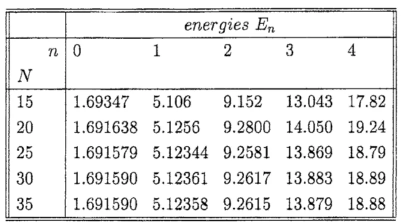
diagonalization. With $s=2$ and $a=c=\beta=\delta=1$, Table 1 illustrates the _practical

implem entation

as

well as the highly satisfactory rate ofconvergence ofthe numerical

HD algorithm.

5.2

Outlook

We have $\mathrm{r}\mathrm{e}$-confirmed that the HD methods bridge

a

gap between the brute-force

present context,

we

emphasized that the HD techniques may be combined not only

with the complexification of the variables (characteristic for the latter approach) but

also with the requirements of a numerical efficiency (pursued, usually, in the former

setting).

In the conclusion

we

may note that another iink connects also theHD and

pertur-bativetechniques. Inthe latter, semi-analytic typeofconsiderations,

an

indispensable

role is played by asymptotic expansions, say, ofthe power-series form

$Z( \lambda)=\sum_{k=0}^{M}\lambda^{k}z_{k}+R_{M}(\lambda)$ (26)

where A represents a- presumably, “sufficiently” small - coupling constant while the

typical example ofthe observabde $Z(\lambda)$ is

a

bound-state energy. In the present HD

setting

we

employed

a

similaransatz (26) where the variable A denoted the coordinate

$x$ while the function $Z(\lambda)$ represented the

wave

function.

Currently, a numerical credibility of the similar perturbative (and also

semi-classical) constructions is being enhanced via

an

improved treatment of the

error

term $R_{M}(\lambda)$

.

In

generat,

this does not seem to be the

case

in the present HD context.

The

reason

is that although forthebound states the exponentially growing right-hand

sum

must be identically zero, we are still not interested in the explicit evaluation of

the exponentially suppressed remainder $R_{\lambda f}(\lambda)$ (which would behopeless) but merely

in the bracketing property ofthe wave-function

sum

$\sum_{k=0}^{M}$$\lambda^{k}z_{k}\neq 0$ evaluated slightly

below and slightly above the actual physical energy.

In this sense,

we

may summarize that the HD “trick” is different and enables

us

to pa$\mathrm{y}$ a

more

detailed attention to the

new

perspectives opened by the consequent

complexification of $\lambda$. Here, such a perspective enabled

us

to extend the standard

mathem atical background ofthe Hill-determinant constructions ofbound states. We

have

seen

that the old principles stay at work, making

use

of the

same

mechanism

as in the standard Hermitian cases, viz, the constructiveiy employed asymptotic

can-cellation of the growing exponentials in the exponentially decreasing

wave

functions

$\psi(x)$.

Acknowledgements

Table

Table 1. The convergence ofHD energies.

References

[1] C. M. Bender and T. T. Wu, Phys. Rev. Lett. 21 (1968)

406

and Phys. Rev. 184

(1969) 1231.

[2] A. Voros, Ann. Jnst. Henri Poincare’ A 39 (1983)211 and J. Phys. A: Math. Gen.

27 (1994) 4653.

[3] S. N. Biswas, K. Datta, R. P. Saxena, P. K.

Srivastava

and V.

S.

Varma, J. Math.

Phys. 14 (1973) 1190; F. T. Hioe, D. MacMillanand E. W. Montroll, Phys. Rep,

43 (1978) 305,

[4] B. Simon, Int. J. Quant. Chem. 21 (1982) 3.

[5] E. Caliceti, S. Graffi and M. Maioli, Commun. Math. Phys.

75

(1980)

51.

[6] M. Znojil, Lett. Math. Phys. 5,

405

(1981) and J. Math. Phys. 29 (1988) 139.

[7] F. M. Fernandez, R. Guardiolaand M. Znojil, Phys. Rev. A 48 (1993)

4170.

[8] M. Znojil, J. Phys. A: Math. Gen, _{31 (1998)}

_3349.

[9] V. Singh, S. N. Biswas and K. Data, Phys. Rev. D18 (1978)

1901.

[11] M. Znojil, Non-variational Matrix Methods in Quantum Theory, INP AS CR Rez, 1993, unpublished.

[12] C. M. Bender and S. Boettcher, Phys. Rev. Lett. 24 (1998)

5243

and J. Phys.

A: Math. Gen.

31

(1998) L273.

[13] M. Znojil, J. Phys. A: Math. Gem, ₃₂ (1999) 7419.

[14] M. Znojil, Rendiconti del Circ. Mat. di Palermo, Ser. II, Suppl. 72 (2004) 211

(math-ph/0104012).

[15] C. M. Bender, D. C. Brody and H. F. Jones, Phys. Rev. Lett. 92 (2004) 119902

(erratum).

[16] M. Znojil, Phys. Lett. A 259 (1999)

220.

[17] B. Bagchi, C. Quesne and M. Znojil, Mod. Phys. LettersA 16 (2001)

2047

(quant-$\mathrm{p}\mathrm{h}/0108096)$.

[18] P. A. M. Dirac, Proc. Roy. Soc. London A 180 (1942) 1; W. Pauli, Rev. Mod.

Phys., 15 (1943) 175;

H. Feshbach and F. Villars, Rev, _{Mod. Phys., 30 (1958) 24; E. P. Wigner, J.}

Math. Phys. 1 (1960) 409; F. G. Scholtz, H. B. Geyer and F. J. W. Hahne, Ann.

Phys. 213 (1992) 74; A. Mostafazadeh, J. Math. Phys. 43 (2002)

2814

and

3944.

[19] C. M. Bender, D. C. Brody and H. F. Jones, Phys. Rev. Lett. 89 (2002) 270401.

[20] M. Znojil, Phys. Lett. A

285

(2001)

7

(quant-ph/0101131).

[21] A. Mostafazadeh and A. Batal, Physical Aspects of Pseudo-Hermitian and

PT-symmetric Quantum Mechanics, quant-ph/0408132.

[22] D. A. Estrin, F. M. Fernandez and E. A. Castro, Phys. Lett. A L30, 330 (1988);

M. Znojil, J. Math. Phys. 33 (1992)

213

and J. Phys. A: Math. Gem. 27 (1994)