Improved
linear
shrinkage
estimators
of large
structured covariance matrices
池田祐樹久保川達也
$\dagger$東京大学
Yuki Ikeda and
Tatsuya
Kubokawa
University
of
TokyoAbstract
The problem of estimating large covariance matrices with use of factor models
is addressed. In this article, we consider a general class of weighted estimators
which includes (i) linear combinations of the sample covariance matrix and the
model-basedestimator under thefactormodel and (ii) ridge-type estimators without
factors
as
specialcases.
The optimal weights in theclassare derived, and theplug-in weightedestimators
are
suggested since theoptimalweights dependon unknownparameters. Some asymptotic arguments
are
given. Numerical results showour
methods perform well under both normal and non-normal distributions.
Key words andphrases: Covariancematrix, factor model, high dimension, large
sample, non-normaldistribution, normal distribution, portfolio management,
ridge-type estimator, risk function.
1
研究の背景と概要
1.1
研究の背景
(1);
高次元共分散行列
$\bullet$ 高次元ベクトル $y_{i}$ の分散共分散行列 $\Sigma_{11}:=Cov(y_{i})$ の推定問題: 次元$p$がサンプル数$N$ を超えるとき逆行列存在せず.$p<N$
でも$p$が相対的に大きいと不安定. $\bullet$ 既存研究 :多数の文献(ここでは特に 2 つ列挙)*Graduate School of Economics, University of Tokyo, 7-3-1 Hongo, Bunkyo-ku, Tokyo 113-0033,
JAPAN, E–Mail: [email protected]
$\dagger$
Faculty of Economics, University of Tokyo, 7-3-1 Hongo, Bunkyo-ku, Tokyo 113-0033, JAPAN,
-weighted estimators(ridge-type estimators);
Ledoit
andWolf
(2004),Schafer and Strimmer
(2005), Chen, Wiesel,Eldar
and
Hero (2010), Kubokawa and
Srivastava
(2013),
$\ldots$$\Sigma_{T}^{8}:=w\hat{\Sigma}_{11}+(1-w)\frac{1}{p}tr(\hat{\Sigma}_{11})I\wedge$, (1.1)
$-regularization/$
thresholding estimators;Bickel
andLevina
$(2008a, 2008b)$, Rothman,Levina and Zhu
(2009),Cai and
Liu
(2011), -他にも Bayse推定量,修正コレスキー分解,行列指数関数
1.2
研究の背景
(2);
ファクターモデル
$\bullet$ その分散共分散行列に興味のある変数 $y_{i}$以外に共変量$x_{i}$が利用可能な場合:(
線形)
ファクターモデル$\bullet$
3-
ファクターモデル(Famaand
French (1993)):$r_{it}=b_{i1}f_{it}+b_{i2}f_{2t}+b_{i3}f_{3t}+u_{it},$
$r_{it}:$
excess
asset
return, $f_{1t}:$sensitivityto
the market
excess
return, $f_{2t}:$market
capi-talization, $f_{3t}:$
book
to-priceratio.
$\bullet$ ファクターモデルにおける高次元共分散行列の推定:
Fan, Fan and Lv (2008)
$\bullet$ 近似ファクターモデルにおける高次元共分散行列の推定:
Fan,
Liao
and
Mincheva
$(2011, 2013)$$\bullet$ これら Fan,
et
al. $(2011, 2013)$ は,Errorcovariance matrix
にthresholding を適用(Error
covariance
matrix にスパース性の仮定).
1.3
研究の背景
(3); weighted
estimators
とファクターモデル
$\bullet$
Ledoit and
Wolf
(2003),Ren
andShimotsu
(2009):$-p$
:
固定,
N
$arrow\infty$(
非高次元)
で,(1) 標本分散共分散行列と (2) ファクターモデルから示唆される推定量の線形結合を提案.
$\bullet$ 本発表
:
$p,$$Narrow\infty$
の高次元の枠組みで,ファクターモデルを利用した線形縮小推定
量 (linearshrinkage, weighted
or
ridge-type
estimators) を提案.$\bullet$
基本的なアイデアは,Ledoit
and Wolf
(2003),Ren and
Shimotsu
(2009) と同様:標本分散共分散行列とファクターモデルが成り立つもとで示唆される推定量の線形
$\bullet$
数値実験の結果,正規非正規分布下で,提案推定量は分散共分散行列だけでなく逆
行列の推定でも,標本共分散行列や Fan,
et
al. (2011) を含む他の推定量に比べ,良い結果を与えた.
2Weighted
Estimators
とその MSE
2.1
Unrestricted model and
Factor model
$\bullet$
$y_{i}\in \mathbb{R}^{p}$
および跳と相関のある共変量
$x_{i}\in \mathbb{R}^{q}$が次のように生成されているとする: $y_{i}\sim i.i.d.(\mu_{1}, \Sigma_{11}) , x_{i}\sim i.i.d.(\mu_{2}, \Sigma_{22})$.
(2.1)ここで跳に関して
$x_{i}$ によるファクターモデルが成り立っていると仮定する:$y_{i}=\alpha+\beta x_{i}+\epsilon_{i},$ $i=1$
,
. . .
,
$N,$(2.2)
$\epsilon_{i}\sim i.i.d.(O, D) , x_{i}\sim i.i.d.(\mu_{2}, \Sigma_{22})$,
$\Sigma_{12}=Cov(y_{i}, x_{i})$
とおくと,上式は次のように書き直することができる.
$y_{i}=(\mu_{1}-\Sigma_{12}\Sigma_{22}^{-1}\mu_{2})+\Sigma_{12}\Sigma_{22}^{-1}x_{i}+\epsilon_{i},$ $i=1$,
.
.
.
,$N,$(2.3)
$\epsilon_{i}\sim i.i.d.(O, D) , x_{i}\sim i.i.d.(\mu_{2}, \Sigma_{22})$,
$\bullet$ 厳密なファクターモデル (strict
factor
model) では$D=dI_{p}$ (sphericity) または
$D=$ diag ($d_{1}, \ldots, d_{p})$(diagonality) を想定.
$\bullet$
すると上のファクターモデルが成り立つならば,
$\Sigma_{11}:=Cov(y_{i})=D+\beta^{T}\Sigma_{22}\beta=D+\Sigma_{12}\Sigma_{22}^{-1}\Sigma_{21}.$
2.2
Weighted
Estimators
$\bullet n=N-1,$ $\overline{y}=N^{-1}\Sigma_{i=1}^{N}y_{i},$ $\overline{x}=N^{-1}\Sigma_{i=1}^{N}x_{i},$ $\hat{\Sigma}_{11}=\Sigma_{i=1}^{N}(y_{i}-\overline{y})(y_{i}-\overline{y})^{T}/n,$ $\hat{\Sigma}_{12^{\wedge}}=\Sigma_{21}^{T}=\Sigma_{i=1}^{N}(y_{i}-\overline{y})(x_{i}-\overline{x})^{T}/n,$ $\hat{\Sigma}_{22}=\Sigma_{i=1}^{N}(x_{i}-\overline{x})(x_{i}-\overline{x})^{T}/n,$ $\hat{\Sigma}_{11.2}=$
$\hat{\Sigma}_{11^{\wedge\wedge-1\wedge}}-\Sigma_{12}\Sigma_{22}\Sigma_{21}.$
.
$\Sigma_{11}$ の推定量$\delta$ は,以下の mean squarederror (MSE) のもとで評価する:$R(\omega, \delta)=p^{-1}E[tr[(\delta-\Sigma_{11})^{2}]],$
ただし$\omega$ は未知のパラメータの組.
$\bullet$
$\bullet$
一方鋤による厳密なファクターモデルが推測されるときには,以下の推定量が自然
:
$\hat{\Sigma}_{f}=\Lambda(\hat{\Sigma}_{11.2})+\hat{\Sigma}_{12}\Sigma_{22}\Sigma_{21}^{\wedge-1\wedge}$
.
(2.4)
ここで$\Lambda$ は$D$ の推定量であり,
(C1)
Case
of sphericity:
$\Lambda(\hat{\Sigma}_{11.2})=p^{-1}tr(\hat{\Sigma}_{11.2})I.$(C2)
Case
of diagonality:
$\Lambda(\hat{\Sigma}_{11.2})=diag(\hat{\Sigma}_{11.2})$.
近似ファクターモデルまで考慮するため,分散共分散行列
$\hat{\Sigma}_{11}$ を,厳密なファクター モデルにおける自然な推定量$\hat{\Sigma}_{f}$ の方向に縮小した以下のような推定量を考える. $\hat{\Sigma}_{\alpha}=\alpha\hat{\Sigma}_{11}+(1-\alpha)\hat{\Sigma}_{f}, \alpha\in[0, 1 ]$.
(2.5)
すると以下のように書き直せる: $\hat{\Sigma}_{\alpha}=\alpha\hat{\Sigma}_{11.2}+(1-\alpha)\Lambda(\hat{\Sigma}_{11.2})+\hat{\Sigma}_{12}\Sigma_{22}\Sigma_{21}^{\wedge-1\wedge}$ . (2.6)$\Sigma_{11.2}$ のsphericity あるいはdaigonalityの度合いが小さくなるほど$\alpha$ は
1
に近づき,$\hat{\Sigma}_{\alpha}$ は単なる標本共分散行列に退化していってしまう。 そこで:以下のようなより広
いクラスを考える
$\hat{\Sigma}(\gamma, \beta)=\gamma\hat{\Sigma}_{11.2}+(1-\gamma)\Lambda(\hat{\Sigma}_{11.2})$
$+\beta\hat{\Sigma}_{12}\Sigma_{22}\Sigma_{21}^{\wedge-1\wedge}+(1-\beta)\Lambda(\hat{\Sigma}_{12}\Sigma_{22}\Sigma_{21}^{\wedge-1\wedge})$
.
(2.7)(C1)
Case
of sphericity: $\Lambda(\hat{\Sigma}_{12}\Sigma_{22}\Sigma_{21}^{\wedge-1\wedge})=p^{-1}tr(\hat{\Sigma}_{12}\Sigma_{22}\Sigma_{21}^{\wedge-1\wedge})I,$(C2)
Case
of diagonality: $\Lambda(\hat{\Sigma}_{12}\Sigma_{22}\Sigma_{21}^{\wedge-1\wedge})=diag(\hat{\Sigma}_{12}\Sigma_{22}\Sigma_{21}^{\wedge-1\wedge})$.
すると $\hat{\Sigma}_{\alpha}$ は,$\gamma=\alpha$ かつ$\beta=1$ に対応する.
とくに(Cl)(sphericity) のケースでは,$\gamma=\beta=w$ とおくと,
Kubokawa
andSrivas-tava(2013) で扱われている共変量をもちいない weighted estimator
$\hat{\Sigma}_{T}=w\hat{\Sigma}_{11}+(1-w)\Lambda(\hat{\Sigma}_{11})I$ (2.8)
になる.
(C1)
Case of sphericity:
$\Lambda(\hat{\Sigma}_{11})=p^{-1}tr(\hat{\Sigma}_{11})I,$(C2)
Case
ofdiagonality:
$\Lambda(\hat{\Sigma}_{11})=diag(\hat{\Sigma}_{11})$.
以下では上の推定量のクラス (2.7) において,MSE を最小にする $\beta$ と
2.3
risk
function
の近似
$\bullet$ ケース
(C1)
または(C2)
のもとで,$\hat{\Sigma}(\gamma, \beta)$ のリスクは以下のように表される:$R(\omega,\hat{\Sigma}(\gamma, \beta))=(\gamma\beta)(\begin{array}{ll}J_{11} J_{12}J_{12} J_{22}\end{array})(\begin{array}{l}\gamma\beta\end{array})-2(J_{10} J_{20})(\begin{array}{l}\gamma\beta\end{array})+R_{0}$, (2.9)
したがって最適なウエイトゲ,
$\beta^{*}$ は$(\begin{array}{l}\gamma^{*}\beta^{*}\end{array})=(\begin{array}{ll}J_{11} J_{12}J_{12} J_{22}\end{array})(\begin{array}{l}J_{10}J_{20}\end{array})$
.
(2.10)で与えられ,これら $\gamma^{*},$$\beta^{*}$ をウエイトに持つ推定量$\hat{\Sigma}(\gamma, \beta)$ のリスクは
$R(\omega,\hat{\Sigma}(\gamma^{*}, \beta^{*}))=R_{0}-(J_{10} J_{20})(\begin{array}{ll}J_{11} J_{12}J_{12} J_{22}\end{array})(\begin{array}{l}J_{10}J_{20}\end{array}),$
$\bullet$ ただし,
(C1)
Case
of
sphericity: $\Lambda(\Sigma_{11})=p^{-1}tr(\Sigma_{11})I,$(C2)
Case of diagonality:
$\Lambda(\Sigma_{11})=diag(\Sigma_{11})$,として, $R_{0}= \frac{1}{p}Etr(\Sigma_{11}-\Lambda(\hat{\Sigma}_{11}))^{2}, J_{11}=\frac{1}{p}Etr(\hat{\Sigma}_{11.2}-\Lambda(\hat{\Sigma}_{11.2}))^{2},$ $J_{22}= \frac{1}{p}Etr(\hat{\Sigma}_{12}\Sigma_{22}\Sigma_{21}^{\wedge-1\wedge}-\Lambda(\hat{\Sigma}_{12}\Sigma_{22}\Sigma_{21}^{\wedge-1\wedge}))^{2},$ $J_{12}=^{\underline{1}}Etr(\hat{\Sigma}_{11.2}-\Lambda(\hat{\Sigma}_{11.2}))(\hat{\Sigma}_{12}\Sigma_{22}\Sigma_{21}^{\wedge-1\wedge}-\Lambda(\hat{\Sigma}_{12}\Sigma_{22}\Sigma_{21}^{\wedge-1\wedge}))$ ,
(2.11)
$p$ $J_{10}=^{\underline{1}}Etr(\hat{\Sigma}_{11.2}-\Lambda(\hat{\Sigma}_{11.2}))(\Sigma_{11}-\Lambda(\Sigma_{11}))$ , $p$ $J_{20}= \frac{1}{p}Etr(\hat{\Sigma}_{12}\Sigma_{22}\Sigma_{21}^{\wedge-1\wedge}-\Lambda(\hat{\Sigma}_{12}\Sigma_{22}\Sigma_{21}^{\wedge-1\wedge}))(\Sigma_{11}-\Lambda(\Sigma_{11}))$.
$\bullet$ 以下,$\Sigma_{11.2}:=\Sigma_{11}-\Sigma_{12}\Sigma_{22}^{-1}\Sigma_{21}$ とする. $\bullet$ 以下では簡単のため,ケース (Cl):sphericity のときのみ考える.$\bullet$ 推定量のリスクを近似するにあたって,以下の (A1) (A2) を仮定し,さらに (A3) ま
たは (A4) のどちらかを仮定する:
(A1) $n,$ $p$
and
$q$satisfy that
$(n,p)arrow\infty,$ $n\geq q$and
$q$is
bounded.
(A2) $a_{1}=p^{-1}tr(\Sigma_{11})=O(1)$, $b_{1}=p^{-1}tr(\Sigma_{11.2})=O(1)$, $b_{2}=p^{-1}tr(\Sigma_{11.2}^{2})=O(1)$
and
$\phi_{11}=p^{-1}tr(\Sigma_{11}\Sigma_{11.2})=O(1)$.
(A3) $a_{2}=p^{-1}tr$$(\Sigma_{11}^{2})=p^{-1}tr$ $(\Sigma_{11.2}+\Sigma_{12}\Sigma_{22}^{-1}\Sigma_{21})^{2}=O(p)$
.
(A4) $a_{2}=O(1)$.
$\bullet$
$x_{i}$, $\epsilon$
i(
したがって$y_{i}$)
に正規性を仮定すれば馬,
$J_{kl}$ が解析的に求まる.$\bullet$ ケース (C1)
のときには,仮定
(A3) または(A4) の下で,$J_{11}=b_{2}-b_{1}^{2}+ \frac{p}{n}b_{1}^{2}+O(n^{-1})+O(n^{-2}p)$, $J_{12}=\phi_{11}-a_{1}b_{1}-b_{2}+b_{1}^{2}+O(n^{-1})$, $J_{10}=\phi_{11}-a_{1}b_{1}+O(n^{-1})$, $J_{20}=a_{2}-a_{1}^{2}-\phi_{11}+a_{1}b_{1}+O(n^{-1})$
.
であり,仮定 (A3) のときは,
$J_{22}=(1+n^{-1})a_{2}-2\phi_{11}+b_{2}-(a_{1}-b_{1})^{2}$ $+ \frac{p}{n}(a_{1}^{2}-b_{1}^{2})+O(n^{-1})+O(n^{-2}p)$, 仮定 (A4) のときには, $J_{22}=a_{2}-2 \phi_{11}+b_{2}-(a_{1}-b_{1})^{2}+\frac{p}{n}(a_{1}^{2}-b_{1}^{2})+O(n^{-1})+O(n^{-2}p)$.
$\bullet$ Risk of $\hat{\Sigma}_{11}$ :簡単な計算から $Ri_{\mathcal{S}}k(\hat{\Sigma}_{11})=a_{2}/n+(p/n)a_{1}^{2}.$ $\bullet$ Riskof
$\hat{\Sigma}_{\alpha}$:ケース(Cl):sphericity のとき,(2.9) 式で$\gamma=\alpha,$ $\beta=1$ とおいて前
ページの式をもちいると $Ri_{\mathcal{S}}k( \hat{\Sigma}_{\alpha})=(b_{2}-b_{1}^{2}+\frac{p}{n}b_{1}^{2})\alpha^{2}-2(b_{2}-b_{1}^{2})\alpha+\frac{a_{2}}{n}$ $+ \frac{p}{n}(a_{1}^{2}-b_{1}^{2})+b_{2}-b_{1}^{2}+O(n^{-1})+O(n^{-2}p)$, となりこれを最小化する $\alpha$ は $\alpha^{*}=\frac{b_{2}-b_{1}^{2}}{b_{2}-b_{1}^{2}+(p/n)b_{1}^{2}}$
.
(2.12) $\Sigma\alpha$。のリスクはRisk
$( \hat{\Sigma}_{\alpha^{*}})=\frac{a_{2}}{n}+\frac{p}{n}a_{1}^{2}-b_{1}^{2}(\frac{p}{n}-\frac{p(b_{2}/b_{1}^{2}-1)}{n(b_{2}/b_{1}^{2}-1)+p})+O(n^{-1})+O(n^{-2}p)$,これは
leading terms
$\#_{\sim}’$おいて $\hat{\Sigma}_{11}$ より小さい.3
Plug-In
推定量の構成
3.1
Plug-In
推定量
$\bullet$ ここまで$\Sigma\alpha$, $\hat{\Sigma}(\gamma,\beta)$
の最適なウエイトを評価してきたが,実際に推定を行うにはこ
$\bullet$
$a_{1},$ $a_{2},$ $b_{1},$ $b_{2}$ に関しては以下の各推定量をもちいる
(Srivastava (2005)):
$\hat{a}_{1}=\frac{1}{p}tr(\hat{\Sigma}_{11}) , \^{a}_{20}=\frac{n}{p(n+2)}tr((diag\hat{\Sigma}_{11})^{2})$, $\^{a}_{2}=\frac{n^{2}}{p(n-1)(n+2)}(tr(\Sigma_{11}^{2})\wedge-(tr\hat{\Sigma}_{11})^{2}/n)$, (3.1) $\hat{b}_{1}=\frac{n}{p(n-q)}tr(\hat{\Sigma}_{11}) , \hat{b}_{20}=\frac{n^{2}}{p(n-q)(n-q+2)}tr((diag\hat{\Sigma}_{11.2})^{2})$, $\hat{b}_{2}=\frac{n^{2}}{p(n-q-1)(n-q+2)}(tr(\Sigma_{11.2}^{2})-\wedge(tr\hat{\Sigma}_{11.2})^{2}/(n-q))$, $\bullet$ また $\phi_{11}$ に関しては以下をもちいる: $\hat{\phi}_{11}=\frac{n}{p(n-q)}(tr(\hat{\Sigma}_{11}\hat{\Sigma}_{11.2})-\frac{n-q-2}{(n-q-1)(n-q+2)}tr(\Sigma_{11.2}^{2})\wedge$ $- \frac{n-q}{(n-q-1)(n-q+2)}(tr\hat{\Sigma}_{11.2})^{2})$
.
$\bullet$ これらを(2.12) に代入することにより,
Plug-In
推定量$\Sigma_{\hat{\alpha}^{*}}$ を提案する.またこれらを 15ページの各$J$の leading terms に代入し、 さらに (2.10) に代入することにより,
$\hat{\Sigma}(\hat{\gamma}^{*},\hat{\beta}^{*})$ を提案する.
3.2
一致性
$\bullet$
さらに以下の条件を仮定し,上述の推定量の一致性に関して議論する
:
(A5) $a_{4}=p^{-1}tr(\Sigma_{11}^{4})=O(p^{3})$, $b_{3}=p^{-1}tr(\Sigma_{11.2}^{3})=O(1)$, $b_{4}=p^{-1}tr(\Sigma_{11.2}^{4})=$
$O(1)$,
tr$(\Sigma_{11.2}\Sigma_{12}\Sigma_{22}^{-1}\Sigma_{21})^{2}=O(p^{2})$
and
tr$(\Sigma_{11.2}^{2}\Sigma_{12}\Sigma_{22}^{-1}\Sigma_{21})=O(p)$.
Theorem
3.1.
Assume
(A1), (A2), (A3) and (A5), then under normality, $\^{a}_{1},$ $\^{a}_{2},$ $\hat{b}_{1},$ $\hat{b}_{2}$and $\hat{\phi}_{11}$
are
all unbiased and$\^{a}_{1}=a_{1}+O_{p}(n^{-1/2}) , \^{a}_{2}=a_{2}+O_{p}(n^{-1/2}p)$
,
$\hat{b}_{1}=b_{1}+O_{p}((np)^{-1/2}) , \hat{b}_{2}=b_{2}+O_{p}((np)^{-1/2})+O_{p}(n^{-1})$,
$\hat{\phi}_{11}=\phi_{11}+O_{p}(n^{-1/2})$
.
4
数値実験
4.1
設定
$\bullet$ データ生成過程:
$y_{i}=\alpha+\Sigma_{12}\Sigma_{22}^{-1}x_{i}+\epsilon_{i}, \epsilon_{i}=\Sigma_{11.2}^{1/2}u_{i}, x_{i}=\Sigma_{22}^{1/2}v_{i}$
ここで$u_{i}=(u_{ij})_{1\leq j\leq p},$ $v_{i}=(v_{ij})_{1\leq j\leq q}$ は互いに独立とする.
$\bullet$ 正規分布(D1)
$u_{ij},$$v_{ij}\sim N(0,1)$
非正規分布$(D2)u_{ij},$$v_{ij}=(w_{ij}-\nu)/\sqrt{2v},$ $w_{ij}\sim\chi^{2}(v)$ かつ $v=2.$
$\bullet$
$\mu_{2}=0,$ $\Sigma_{22}=I_{q},$ $(\Sigma_{12})_{ij}\sim i.i.d.$ $\mathcal{N}(0.5,1)$
.
$\bullet$ 厳密なファクターモデル $(M1):\Sigma_{11.2}=3I,$
近似ファクターモデル (M2):
$\Sigma_{11.2}=(\begin{array}{llll}\sigma_{1} \sigma_{2} \ddots \sigma_{p}\end{array})(\begin{array}{llll}\rho^{|1-1|/7}\rho^{|2-1|/7} \rho^{|1-2|/7}\rho^{|2-2|/7} .\cdot \rho^{|1-p|/7}\rho^{|2-p|/7}\vdots \vdots \rho^{|p-1|/7} \rho^{|p-2|/7} .\cdot \rho^{|p-p|/7}\end{array})(\begin{array}{llll}\sigma_{1} \sigma_{2} \ddots \sigma_{p}\end{array}),$
ただし $\sigma_{j}=3+0.2(-1)^{j-1}(p-i+1)/P$かつ $\rho=0.2.$
$\bullet 7$ つの推定量$\hat{\Sigma}_{11},$ $\Sigma_{T}^{s}^{\wedge},$ $\Sigma_{T}^{d}^{\wedge},$ $\Sigma_{\hat{\alpha}^{*}}^{s}^{\wedge},$ $\Sigma_{\hat{\alpha}^{*}}^{d}^{\wedge},$
$\Sigma^{8}(\hat{\gamma}^{*},\hat{\beta}^{*})\wedge,$ $\Sigma^{d}(\hat{\gamma}^{*},\hat{\beta}^{*})\wedge 1$を比較.各々 1000 回
繰り返し,次のロスで計算される経験リスクと対応する標準偏差を計算した.
$\bullet$ $\Sigma_{11},$ $\Sigma_{11}^{-1}$
の推定に関して,それぞれ以下で評価.
$p^{-1}tr[(\delta-\Sigma_{11})^{2}]$
for
$\Sigma_{11},$ $p^{-1}tr[(\delta\Sigma_{11}-I)^{2}]$for
$\Sigma_{11}^{-1}.$$\bullet$ $N=100,$ $q=3$ と固定し、$p=50$, 100, 200とした。
4.2
Numerical Results
末尾のTable 1-4に示している.
1添え字の $s,$ $d$はそれぞれ (C1):sphericity, (C2):diagonality を示す.$\hat{\Sigma}_{T}$ は
5
結論
5.1
議論
$\bullet$ リスクの近似の計算で、$O_{p}(n^{-2}p)$ の項が出てくるため、 この項が無視できないほど
$P$が大きいときは、 誤差が生じてくる。
$-$
ファクターローディング
(factor
loadings)
$\Sigma$12$\Sigma$
2-21
$($ したがって$a_{2}=tr\Sigma_{11}^{2}/p)$ の密度が$\^{a}_{2}$ の収束レートに深くかかわっている.
$-(A4)a_{2}=O(1)$ のときは仮定 (A5) において $a_{4}=p^{-1}tr(\Sigma_{11}^{4})=O(1)$ と修正し
ても非整合的ではなく,
$(np)^{-1/2}arrow 0$のとき $\hat{a}_{2}$ は一致性をもつ.$\bullet$ $(A3)tr\Sigma^{2}=O(p^{2})$ のもとでは漸近的には
$|\gamma^{*}-\alpha^{*}|arrow 0,$ $\beta^{*}arrow 1$
となるので,漸近的
に $\Sigma_{\gamma,\beta}$ と $\Sigma_{\alpha}$ のリスクは等しくなる。$(A4)tr\Sigma^{2}=O(p)$ のもとでは漸近的にも $|$ゲー$\alpha^{*}|arrow 0,$ $\beta^{*}arrow 1$
となり,漸近的にも
$\Sigma_{\alpha}$ に対する $\Sigma_{\gamma,\beta}$ のリスクの改善がみられる.
$\bullet$ 縮小ターゲット$:(tr\hat{\Sigma}/p)I_{p}$
, diag$\Sigma$
5.2
結論
$\bullet$ 本発表で$\ovalbox{\tt\small REJECT}\lambda$
, 高次元の枠組みにおいて $y_{i}$ の共変量$x_{i}$
が得られるときに,
$y_{i}$ の標本共分散行列$\hat{\Sigma}_{11}$ を
$x_{i}$
によるファクターモデルを仮定したもとで示唆される推定量
$\hat{\Sigma}_{f}$の方向へ縮小したクラスの推定量を考え,さらにそれを含むより一般化した推定量
$\hat{\Sigma}(\gamma, \beta)$ のリスクを
Mean Squared Error
の下で調べた.$\bullet$
数値計算の結果,
$y_{i},$ $x_{i}$の正規性のあるなしに関わらず,厳密な
/
近似ファクター
$\acute{}$ モ デルのもとで、$\hat{\Sigma}(\gamma, \beta)$は分散共分散行列,逆行列の推定で,ともに良い結果を与え
ている. $\bullet$同じく数値実験により,ポートフォリオの分散上限制約下で期待リターンの最大化
問題を考えたところ,提案する推定量が制約を守りやすいことがわかった.
$\bullet$全体に正規性に依拠した枠組みであることから、
非正規の場合の推定向上が課題で ある。References
$\bullet$ Bai, Z., Huixia,
L., and Wing-Keung, W. (2009). Enhancement of the applicability of
markowitz’s portfolio optimization by utilizing random matrix theory. Math. Finance,
19,
639-667.
$\bullet$ Bickel, P., and Levina, E. (2008a).
Covariance regularization by thresholding. Ann.
Bickel, P., and Levina, E. (2008b). Regularized estimation of large covariance matrices.
Ann. Statist., 36, 199-227.
Cai, T., and Liu, W. (2011). Adaptive thresholding for sparse covariance matrix
estima-tion. J. Amer. Statist. Assoc., 106,
672-684.
Chen, Y., Wiesel, A., Eldar, C.Y., and Hero, A.O. (2010). Shrinkage Algorithms for
MMSE Covariance Estimation. IEEE Trans. on $Sig$
.
Process., 58,5016-5029.
Fama, E., andFrench,K. (1993). Commonriskfactors in the returnsonstocks and bonds.
J. Financial Economics 33, 3-56.
Fan, J., Fan, Y., and Lv, J. (2008). High dimensional covariance matrix estimation using
a factor model. J. Econometrics, 147, 186-197.
Fan, J., Liao, Y., and Mincheva, M. (2011). High dimensional covariance matrix
estima-tion in approximate factormodel. Ann. Statist., 39,
3320-3356.
Fan, J., Liao, Y., and Mincheva, M. (2013). Large covariance estimation by thresholding
principal orthogonal complements. J. Royal Statist. Soc., 75,
603-680.
Kubokawa, T., and Srivastava, M.S. (2013). Optimal ridge-type estimators ofcovariance
matrix in high dimension. Discussion Paper Series, CIRJE-F-906.
Ledoit, O., and Wolf, M. (2003). Improved estimation ofthe covariance matrix of stock
returns with
an
applicationto portfolio selection. J. EmpiricalFinance, 10,603-621.
Ledoit, O., and Wolf, M. (2004). A well-conditioned estimator for large-dimensional
covariance matrices. J. Multivariate Analysis, 88, 365-411.
Ren, Y.,andShimotsu, K. (2009). Improvement infinitesampleproperties of the
Hansen-Jagannathan distance test. J. EmpiricalFinance, 16, 483-506.
Rothman, A., Levina, E., and Zhu,J. (2009). Generalizedthresholding oflargecovariance
matrices. J. Amer. Statist. Assoc., 104,
177-186.
Schafer, J., and Strimmer, K. (2005). An empirical bayes approach to inferring large-scale
a gene association networks. Bioinformatics, 21, 754-764.
Srivastava, M.S. (2005). Sometests concerning the covariance matrix in high dimensional
Table 1: Comparison of Estimators of
$\Sigma_{11}$under
Strict Factor Model
(M1)$\overline{\overline{50(D1)22622720.018718.9}}pdist.\hat{\sum_{24.5}}\Sigma^{\wedge s}.\Sigma^{\wedge d}.\Sigma^{s}^{\wedge}\sum_{202}^{\wedge s}.\Sigma^{\wedge d}(\gamma.’\beta)\Sigma^{d}^{\wedge}(\gamma, \beta)$
$\frac{(7.1)(6.6)(6.6)(7.1)(7.1)(6.4)(6.4)}{100(D1)47.342.943.038.438.635.435.7}$ $\frac{(12.3)(9.9)(9.9)(12.3)(12.3)(9.8)(9.8)}{200(D1)93.985.986.076.276.470.871.0}$ $\frac{(23.1)(19.2)(19.2)(23.1)(23.1)(18..8)(18.8)}{50(D2)38.234.734.933.233.930531.2}$ $\frac{(27.2)(21.7)(21.7)(27.3)(27.2)(22.0)(22.3)}{100(D2)75.268.468.665.866.560.561.2}$
(49.6)
(38.9)
(38.9)
(49.7)
(49.7)
(39.6)
(39.9)
200
(D2)
158.3
142.7
142.9
140.1
140.8
127.5
128.3
(93.8) (71.7) (71.7) (94.0)(93.9)
(73.4) (73.6)Table 2:
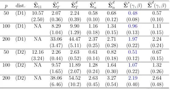
Comparison of Estimators of
$\Sigma_{11}^{-1}$under Strict Factor Model
(M1)$\overline{\overline{50(D1)10.572.072.240.580.68048057}}pdist.\hat{\Sigma}_{11TT\alpha\alpha}\Sigma^{\wedge}\Sigma^{\wedge d}\Sigma^{\wedge}\Sigma^{\wedge}\Sigma^{s}(.\gamma, \beta)\Sigma^{s}(.\gamma, \beta)d\wedge s\wedge d$
(2.50) (0.36) (0.39) (0.10) (0.12)
(0.08)
(0.10)100
(D1)
NA
8.29
9.90
1.16
1.34
0.96
1.11
(1.04) (1.29) (0.18) (0.15) (0.13) (0.15)200
(D1)NA
33.06
44.47
2.37
2.71
1.97
2.24
(3.47) (5.11) (0.25) (0.28) (0.22) (0.24)50
(D2)12.16
2.26
2.63
0.61
0.82
0.51
0.67
(3.24) (0.44) (0.52) (0.14) (0.18) (0.12) (0.15)100
(D2) NA9.57
11.89
1.28
1.64
1.07
1.32
(1.65) (2.07) (0.24) (0.30) (0.22) (0.26)200
(D2)NA
38.06
54.52
2.63
3.27
2.19
2.64
(6.46) (10.2) (0.45) (0.54) (0.40) (0.48)Table
3:
Comparison of
Estimatorsof
$\Sigma_{11}$under Approximate Factor Model
(M2)$\overline{\overline{\overline{50(D1)90088189.6}}p11\wedge\wedge\wedge d\wedge d\wedge\wedge dTT\alpha\alpha}$
(19.0) (15.6) (15.7) (17.1) (17.2) (15.6) (15.6) 100 (D1) 175.3 144.2 145.4 147.0 148.4 138.5 140.1 (26.7) (19.2) (19.2) (23.1) (23.0) (18.9) (18.9) 200 (D1) 338.5 262.6 263.7 257.1 258.6 235.2 236.9 (37.1) (28.2) (28.2) (34.0) (33.9) (25.6) (25.6) 50 (D2) 108.0 90.5 92.2 96.6
98.4
90.8
92.7 (29.8) (20.5) (20.6) (26.2) (26.2) (20.9) (21.2) 100 (D2) 212.6 171.3 173.1 181.3 183.5 166.2 168.8 (65.3) (40.3) (40.4) (62.2) (62.1) (43.0) (43.5) 200 (D2) 410.8 325.5 327.3 325.7 328.3 296.5 299.4 (125.7) (79.6) (79.6) (120.1) (120.2) (84.8) (85.3)Table
4:
Comparison of Estimators of
$\Sigma_{11}^{-1}$under Approximate Factor Model
(M2)$\overline{\frac{\underline{pdist.\bigwedge_{11TT\alpha\alpha}_{\Sigma^{\bigwedge}}\Sigma^{s}\Sigma\Sigma^{\wedge s}\Sigma\Sigma(\gamma,\beta)\Sigma(}.\gamma,\beta)\wedge\wedge d\wedge d\wedge s\wedge d}{50(D1)21.921.291.421.511.711.15130}}$
(4.97) (0.17) (0.19) (0.19) (023)(014) (0.17)