離散方程式の予測への応用 (可積分系研究の新展開 : 連続・離散・超離散)

離散方程式の予測への応用

(Application ofdiscrete equationsto forecasting)

NTTサービスインテグレーション基盤研究所 佐藤大輔 (Daisuke SATOH)

NTT

Service

Integration Laboratories

1

Introduction

From the end of the 1990’s, discrete integrable

equations have been appearing in many fields, e.g., algorithms and traffic flow [17, 18, 19, 20, 34]. Discrete integrable systems

are

expected

to be applied to engineering.

Forecastingis important in engineering. The

making of decisions in various industries is

heavily reliant on forecasting. Forecasting is

the dominant factor in decisions

on

how many

finished products should be made, how much

stock should be prepared and

so on.

In the

past there has been

a

tendency for forecasts to

be unduly optimistic. This has produced

some

serious problems. Therefore, the accuracy of

forecasting is ofgreat importance.

Growth

curve

models

are

used for

forecast-ing in many fields, e.g., ecology [3, 25, 35],

agriculture [26], life sciences [13], marketing

[1, 12], and software reliability growth models

(SRGMs) [14, 22, 36]. To forecast the ceiling,

weestimate parameters of the differential

equa-tion which provides the growth

curve

model.

The differential equations which

are

used

gen-erallyhave exact solutions. Intheconventional

method, the differential equation’s parameters

are

estimated by using

an

ordinary forward

or

central difference equation

as

its

approxima-tion. Generally, the ordinaryforward

or

central

difference equation does not have an exact

so-lution. Therefore, the difference equation does not

conserve

the properties of the differential

equation.

Although

a

growth

curve

model has

practi-cal applications,

one

generally known point is

that the model does not provide accurate

pa-rameterestimatesusingthe dataavailable

dur-ing the early phases ofthe process being

fore-cast. The conventional method is only capable

ofproviding

accurate

estimates of parameters

at the end of the phase. For forecasting to be

ofpractical value, accurate estimates must be

obtained early in the phase.

In this paper, the application of discrete

in-tegrable equations to forecasting is discussed.

We focus

on

discrete integrable analogues of

the logistic equation, the Gompertz equation,

and the Riccati equation forforecasting in two

fields: marketing andSRGM.Theremainder of

thispaperis organized

as

follows. FromSect. 2

to Sect. 4 and in

Sect.

6,

we

consider the fore-casting of numbers of software faults

or

soft-ware

failures through

an

SRGM.

In Sect. 2,

we

describe discrete analogues of

the logistic

curve

model [30], which has been

observed in the testing of software systems

[23, 27]. The model is described by either of

two difference equations, which

were

proposed

byMorishita [15] and Hirota [5,6], respectively.

We will

see

that both models yield accurate

pa-rameter estimates,

even

when there is only

a

small amount of input data from actual

soft-ware

testing.

Although the logistic

curve

model is

one

of

the S-shaped SRGMs, S-shaped software

relia-bility growth for actual projects is often

more

closely described by the Gompertz

curve

than

by the logistic

curve

[2, 8, 21]. In Sect. 3,

we

consider the Gompertz

curve as an

SRGM.

Firstly,

we

propose adiscrete Gompertz

equa-tion [28] that has

an

exact solution. We will

see

that the proposedmodelprovidesaccurate

esti-mates of parameters, enabling prediction early

in the testing phase of when the software will

be fit for release.

There is

a

furtherproblemforsoftware

engi-数理解析研究所講究録 1302 巻 2003 年 116-136

neers

and managers: they have had little

guid-ance astowhich models

are

likely to be best for

a

particular application. InSect. 4,

we

propose

a

criterion [31], together with

a

discrete SRGM,

for determining the absolute worth of

a

model.

In Sect. 5, we consider the Bass model,

which is the main impetus underlying behind

the recent diffusionresearch in marketing. The

author has previously proposed adiscrete form

of the Bass model [29]. This model provides

more

accurate estimates of parameters than

is possible with the conventional Bass model.

Furthermore, parameter estimation of the

dis-crete Bass model

overcomes

the three

short-comings of parameter estimation by the

con-ventional (continuous) Bass model: the

time-interml bias, standard error, and

multicolin-earity.

The proposed models yield accurate

aeti-mates ofparameters,

even

fromsmall amounts

ofinput data. These models, however,

are

de

terministic equations,

so

they do not yield dis-tributions oftheestimates. In Sect. 6,

we

Pro-pose

a

discrete stochastic logistic equation that

have

an

exact solution and describe

an

SRGM

that is based

on

this equation. This model

yields distributions of

an

estimate along with

the aetimatae themselves.

Finally, in Sect. 7,

we

summarizethe raeults

of this paper.

2

Logistic

curve

model

2.1

Conventional

logistic

curve

model

The logistic

curve

model is described

as

$\frac{dL(t)}{dt}=\frac{\alpha}{k}L(t)(k-L(t))$

,

(1)

where $L(t)$ is the cumulative number of

soft-ware

failures occurred upto testing time $t$ and

$\alpha$ and $k$

are

constant parameters to be

esti-mated through regression analysis.

A solution ofEq. (1) is given by

$L(t)= \frac{k}{1+m\exp(-\alpha t)}$, (2)

where $k>0,$ $m>0,$and$\alpha>0.$ The parameter

$k$ represents the total number of potential

soft-ware

failures occurring

over an

infinitely long

duration

or

the initial number of faults

inher-$\mathrm{e}\mathrm{n}\mathrm{t}$ in the software system.

2.1.1 Conventional parameter

estima-tion 1

Regression analysis is generally used to

esti-mate total numbers of potential software fail-ures, although there is

a

further conventional method of estimation, which is described in

Sect. 2.1.2.

We take the following regression equation:

$\mathrm{Y}_{n}=A+BL_{n}$, (3)

where

$t_{n}$ $=$ $n\delta$, (4)

$L_{n}$ $=$ $L(n\delta),$ and (5)

$\mathrm{Y}_{n}$ _$=$ $\frac{\frac{L_{n\dagger 1}-L_{n-1}}{2\delta}}{L_{n}}$

.

(6)

Here, $\delta$ is

a

constant difference interval.

Givenregressioncoefficients$\hat{A}$

and $\hat{B},$ where

$\hat{A}$

means

the vaJue of _$A$

as

aetimated through

regressionanalysis, aetimates of the parameters

$k,$$\alpha,$ and$m$

can

be obtained

as

$\hat{k}$ $=$ $\frac{\hat{A}}{\hat{B}’}$ (7) $\hat{\alpha}$ $=$ $\hat{A}$, and (8) $\hat{m}$ _$=$ $\frac{\sum_{n=1}^{N}(\hat{k}-L_{n})}{\sum_{n=1}^{N}(L_{n}\exp(-\hat{\alpha}t_{n}))}$

.

(9) These estimataedepend

on

thedifference

inter-$\mathrm{v}\mathrm{a}\mathrm{l}\delta,$ because Eq. (6) depends

on

$\delta$

.

The accuracy of estimatae thus derived is

said to be poorwhen thereareonly afew data

points. For accuracy,

we

require data points

up to at least

one

point after the point of

in-flection $(t_{n}= \underline{1}_{\mathrm{L}}\mathrm{o}m_{-,L_{n}}\alpha=\frac{k}{2}).$ We

can

judge

whether the obtained data includae the point

ofinflection by checking whether

or

not $\frac{\overline{k}}{2}<L_{n}$

is satisfied, where $\overline{k}$

is predicted empiricauy

or

statistically.

For the estimatae of parameters to be

reli-able, the following condition must be

satisfied:

$w\overline{k}<L_{n}$, (10)

where $\overline{k}$

is predicted empirically

or

statistically

2.2

Discrete

logistic

curve

models

and $w$ is

a

constant parameter, the value of

Two discrete analoguesofthedifferential

equa-which is empirically chosen from the range 0.6

tion (1) for the logistic

curve

model have

al-to 0.8 [14].

ready been proposed. We propose a regression

equation that is appropriate for the estimation

2.1.2 Conventional parameter estima- _{ofparameter for use with these equations.}

tion 2

Another conventional method of estimation is

based

on a

modified exponential

curve

model

[24]. This model is described

as

$y=cf$ ba. (11)

We rewrite the logistic

curve

model

as

$\frac{1}{L(t)}=\frac{1}{k}+\frac{m}{k}\exp(-\alpha t)$

.

(12)

This equation is in the form of the modified

exponential

curve

model.

When it is possible to place

a

model in

this form, parameters $a,b,$ and$c$

are estimated

throughthefollowingmethodof estimation. At

first,

we

divide thedata set into three subsets,

each of which has the

same

number of data

points. If the number of data points is not $\mathrm{a}$

multiple of three,

we

discard the first

one or

two points. Then

we

sum

up the data in each

subset. Finally, parameters $a,$$b,$ and $c$

are

ob-tained as,

$a$ $=$ $( \frac{S_{3}-S_{2}}{S_{2}-S_{1}})$ , (13) $b$ $=$ $(S_{2}-S_{1}) \frac{a-1}{(a^{n}-1)^{2}}$, (14)

$c$ $=$ $\frac{1}{n}\{S_{1}+(S_{1}-S_{2})\frac{1}{a^{n}-1}\},$ (15)

where$S_{1},$ $S_{2},$ and $S_{3}$ represent thesummations

of all elements of the first, second, and third

subsets of the data, respectively, and $n$

repre-sents the numberofdata points in each of the

subsets.

We then obtain estimates ofthe parameters

$k,$_$\alpha,m$ byusing these estimators:

$k$ $=$ $\frac{1}{c’}$ (16)

$\alpha$ $=$ $-\log a,$ and (17) $m$ $=$ $\frac{b}{c}$

.

(18)

2.2.1 Discrete logistic

curve

model with

Morishita’s equation

Morishita [15] proposed the followingequation

as a

discrete form ofEq. (1):

$L_{n+1}-L_{n}= \delta\frac{\alpha}{k}L_{n\dagger 1}(k-L_{n})$

.

(19)

It has

an

exact solution:

$L_{n}= \frac{k}{1+m(1-\delta\alpha)^{t}\star}$, (20)

where $t_{n}=n\delta$

.

Let $\alpha_{\mathrm{c}}=\alpha$ in Eq. (2), and let $\alpha_{dm}=\alpha$ in

Eq. (20). Comparing$\mathrm{E}\mathrm{q}\mathrm{s}$

.

(2) and (20),

we

get

$\alpha_{\mathrm{c}}=-\frac{1}{\delta}\log(1-\delta\alpha_{dm})$

.

(21)

Toderive theregression equation for the

pa-rameters $k,\alpha_{dm},$ and _$m,$

we

rewrite Eq. (19)

as

$\mathrm{Y}_{n}=A+BL_{n+1}$, (22) where $\mathrm{Y}_{n}$ _$=$ $\frac{L_{n+1}}{L_{n}}$, (23) $A$ $=$ $\frac{1}{1-\delta\alpha_{dm}’}$ (24) $B$ $=$ $- \frac{\delta\alpha_{dm}}{k(1-\delta\alpha_{dm})},$ and (25) $t_{n}$ $=$ $n\delta$

.

(26)

Parameters $k,$ $\alpha,$ and $m$

are

estimated by

$\hat{k}$

$=$ $\frac{1-\hat{A}}{\hat{B}}$, (27) $\delta\hat{\alpha}_{dm}$ _$=$ $1- \frac{1}{\hat{A}}$, (28)

$\hat{m}$ _$=$ $\frac{\sum_{n=1}^{N}(\hat{k}-L_{n})}{\sum_{n=1}^{N}(L_{n}(1-\delta\hat{\alpha}_{dm})^{n})}$, (29) where$\hat{A}$and$\hat{B}$

are

the aetimates ofparameters

$A$ and _$B,$ respectively.

$\mathrm{Y}_{n}$ in Eq. (22) is independent of the

differ-ence interval $\delta,$ because $\delta$ is not used in this

equation. The estimates of$\hat{k},$ $\delta\hat{\alpha}_{dm},$ and $\hat{m}$

are

the

same

whatever value of$\delta$ we choose.

2.2.2 Discrete logistic curve model with

Hirota’s equation

Hirota $[5, 6]$ discretized Eq. (1)

as

$L_{n+1}-L_{n}= \delta\frac{\alpha}{k}L_{n}(k-L_{n+1})$

.

(30)

He gave this exact solution:

$L_{n}= \frac{k}{1+m(\frac{1}{1+\delta\alpha})\# t}$, (31)

where $t_{n}=n\delta$

.

Let $\alpha_{dh}=\alpha$ in Eq. (31). Comparing Eqs.

(2) and (31),

we

get

$\alpha_{\mathrm{e}}=\frac{1}{\delta}\log(1+\delta\alpha_{dh})$

.

(32)

To derive the regression equation for

param-eters $k,$$\alpha,$ and $m,$

we

rewrite Eq. (30)

as

$\mathrm{Y}_{n}=A+BL_{n+1}$, (33) where $\mathrm{Y}_{n}$ _$=$ $\frac{L_{n+1}}{L_{n}}$, (34) $A$ $=$ $\delta\alpha_{dh}+1$, (35) $B$ $=$ $- \frac{\delta\alpha_{dh}}{k},$ and (36) $t_{n}$ $=$ $n\delta$

.

(37) The estimates of parameters $k,$ $\alpha,$ and $m$

are

given

as

by $1-\hat{A}$ $\hat{k}$ $=$ $\overline{\hat{B}}$, (38) $\delta\hat{\alpha}_{dh}$ _$=$ $\hat{A}-1$, (39) $\hat{m}$ _$=$ $\frac{\sum_{n=1}^{N}(\hat{k}-L_{n})}{\sum_{n=1}^{N}(L_{n}(\frac{1}{1+\delta\alpha_{\hat{d}h}})^{n})}$, (40)

where$\hat{A}$and $\hat{B}$

are

the aetimatesof

parameters

$A$ and _$B,$ respectively.

$\mathrm{Y}_{n}$ in Eq. (33) is independent of the

differ-ence

interval $\delta$ because $\delta$ is not used in Eq.

(33). The

same

estimates of $\hat{k},$ $\delta\hat{\alpha}_{dh},$ and $\hat{m}$

are obtained, whatever value of$\delta$ we choose.

The regression equation (33) is the

same as

Eq. (22). Moreover, the

same

estimate of k is

given by both equations. Though the estimate

of $\alpha$ depends on discrete equations, both

dis-crete equations yield the

same

estimate of $\alpha_{c}$

.

The

same

estimate ofm is obtained because

$1- \delta\alpha_{dm}=\frac{1}{1+\delta\alpha_{dh}}=\exp(\alpha_{c})=\frac{1}{\hat{A}}$

.

(41)

Therefore, the models with Morishita’s and

Hi-rota’s equations both give the

same

vaJue$\mathrm{o}\mathrm{f}L_{n}$

.

2.3

Parameter

estimation in

the

$1\mathrm{r}$

gistic

curve

models

We compared the accuracy of parameter

esti-mation for the first conventional logistic

curve

model and the discrete logistic

curve

modek.

To compare only the accuracy of parameter

estimation,

we

evaJuated the performance of

the parameter estimates when the data

repre-sented an exact solution of the logistic

equa-tion. We did not consider the second

conven-tional method of parameter estimation,

as

$\mathrm{d}\triangleright$

scribed inSect. 2.1.2, because it inherently $\mathrm{r}\mathrm{e}$

produced the target values ofthe parameters

when given data that

were

an

exactsolutionof

the logistic equation.

We prepared data that represented exact

so-lutions ofthe logistic equation for

a

set of

pe-riods ($t=0$ to 21). We set $k=100,$ $\alpha=0.8$,

and $m=999$

as

the target values. This data

was

inflected at the point where $t^{*}=8.63$ and

$L(t^{*})=50.$ In

our

eduation,

we

setthe

differ-ence

intervalto 1. Weanalyzedfour sets ofthis

data: the three data sets that covered

an

data

uP to (i) the ceiling $(t=0,1, \ldots,21),$ $(\mathrm{i}\mathrm{i})$ just

after the point of inflection $(t=0,1, \ldots,9)$,

(iii) just before the point of inflection $(t=$

$0,1,$_$\ldots,$$8),$ and (iv) the set of the first three

data points(t $=0,1,2$).

The results of

our

comparison

are

shown in

Table 1. Since

we

used

an

exact solution

as

the input data,

an

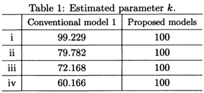
accurate method of

aetima-tion shouldreproduce the parametersthat gen-erated this solution. Table1shows that the

proposed modek estimated $k$ correctly,

even

when the data set only consisted of the first

Table 1: Estimated parameter k.

Conventional model 1 Proposed models

$\mathrm{i}$ 99.229 100 $\mathrm{i}\mathrm{i}$ 79.782 100 $\mathrm{i}\mathrm{i}\mathrm{i}$ 72.168 100 $\mathrm{i}\mathrm{v}$ 60.166 100

four points. Theconventional model had lower

accuracy, despite the

use

of exact solutions to the differential equation

as

data values. As

was

earlierstated, theconventional model is

gener-ally known to providepoorestimates of the

pa-rameters in the situation represented by data

sets (iii) and (iv), $\mathrm{i}.\mathrm{e}.,$ when the data set does

not include the data points around the point of inflection. Empirical studies have shown that

stable and robust estimates of the parameters

of SRGMs, such

as

the logistic

curve

model,

cannot be obtained without using data points

that

cover

thepointof inflection and satisfyEq.

(10), $\mathrm{i}.\mathrm{e}.,$$w\overline{k}<L_{n}.$ Even when dataset (ii)

was

used, the conventional method provided

esti-mates the parameter values that

were

neither

stable nor robust,

even

though set (ii) both

in-cludes the point of inflection and satisfies Eq.

(10).

We evaluated the discrete logistic

curve

$\mathrm{m}\mathrm{o}\mathrm{d}-$

els

on an

actual data set to show that they

are more

appropriate to

use

than the

conven-tional model. The data

were

debugging data

for

an

item ofsoftware. We evaluated the pa-rameter aetimatesgiven both with alldata and

with only that data available early in the

test-$\mathrm{i}\mathrm{n}\mathrm{g}$phase. In

our

evaluation,

we

set

$\delta$ equalto

1. Figure1 showsresults for the ‘all data’ case;

we see

that having all of the data leads to all

three models fitting the actual data very well.

Moreover, the discrete logistic

curve

models

have the important advantage of providing

ac-curate parameter estimates early in the testing

phase

as

well

as

atthe endofthe testing phase.

Therefore, the accuracy of

an

SRGM’$\mathrm{s}$

param-eter estimates early in the testing phase is

an

important aspect ofits utility

as an

estimator.

The

accuracy

of parameter $k$ is especially

im-portant, because this parameter indicates the

15 $\alpha$ $\infty$ $u$ 43 $\infty$ 57 $u$ 71 $7l$ $u$ $n$ $\mathfrak{B}$

Time of observ#on

Figure 1: Comparison the three models with

actual data.

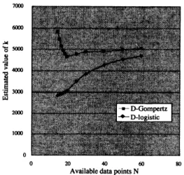
Figure 2: Parameter estimates of$k$

.

potentialfault content of the software system.

To compare the conventional and proposed

modelsin terms ofthis property,

we

estimated

values of $k$ from increasing number of data

points, starting with asmall amount of data

ffom the earlier part of the testing phase. As

is shown in Fig. 2, the values of$k$estimated by

the proposed modelswerestabler than those

es-timated by the conventional models. Since the

proposed models provide

more

accurate

esti-mates of parameter values ffom small amounts

ofdatagatheredearly inthe testing phase, they

providebetter estimatesof totalnumbersof$\mathrm{p}\mathrm{c}\succ$

tential software failures, $k,$ early in the testing

phase.

3

Gompertz

curve

model

3.1

Conventional

Gompertz

curve

model

The Gompertz

curve

model is described

as

$\frac{dG(t)}{dt}=G(t)(\log a)(\log b)b^{t}$ ₍₄₂₎

or

$\frac{dG(t)}{dt}=(\log b)G(t)\log\frac{G(t)}{k}$, (43)

where $G(t)$ is the cumulative number of

soft-ware

failures detected up to atesting time $t$

.

By integrating either equation and assuming

that $G(0)=ka,$ $G(t)$ can be written as

$G(t)=ka^{b^{t}}$

$(k>0,0<a<1,0<b<1)$

_,

(44)

where $a,$ $b,$ and $k$

are

parameters whose

con-stant valuae

are

estimated by using regression

analysis. Parameter $k$ repraeents the total

number of software failures with the potential

to

occur over an

infinitely long period

or

the

initial fault content in the softwaresystem:

$G(t)arrow k(tarrow\infty)$

.

(45)

3.1.1 Conventional parameter estima-tion 1

Regression analysis is generally used to

esti-mate total numbers ofpotential software fail-ures, although

we

also have the conventional

method of estimation that is shown in

Sect.

3.1.2.

The following _{regression equation is}

ob-tained:

$\mathrm{Y}_{n}=A+Bn$, (46)

where

$\mathrm{Y}_{n}$ _{$=$ $\log(\frac{G_{n+1}-G_{n-1}}{2\delta G_{n}})$} , (47) $A$ _{$=$ $\log((\log a)(\log b)),$} and (48)

$B$ $=$ Jlog$b$

.

(49)

Givenregraesioncoefficients$\hat{A}$

and$\hat{B}$

, where$\hat{A}$

means

the parameter $A$

as

estimated through

regression analysis,

we

have these estimators

for parameters $a,$ $b,$ and $k$:

\^a $=$ $\exp(\frac{\delta\exp\hat{A}}{\hat{B}})$ , (50)

$\hat{b}$

$=$ $\exp(\frac{\hat{B}}{\delta}),$ and (51)

$\hat{k}$

$=$ $\frac{\sum_{n=1}^{N}G_{n}}{\sum_{n=1}^{N}\hat{a}^{\hat{b}^{\delta n}}}$

.

(52)

These estimates depend

on

thedifference

in-terval $\delta,$ because $\mathrm{Y}_{n}$ in Eq. (46) depends

on

J.

We

can

choose any value

as

$\delta.$ Therefore, the

estimates

are

entirely dependent

on

the specific

value of$\delta$

.

Theaccuracyof thaeeestimatesispoorwhen

there

are

only

a

few data points. We need data up to at least

one

point afler the point of

in-flection to get accurate aetimates. Afurther condition must be satisfied:

$w\overline{k}<G_{n}$, (53)

where $\overline{k}$

and $w$

are

the

same as

in the

case

of

the logistic

curve

model.

3.1.2 Conventional parameter $\mathrm{e}\mathrm{s}\mathrm{t}\mathrm{i}\mathrm{m}\mathrm{a}-$

tion 2

(55)

The other method of aetimation is the

same as

that ofSect. 2.1.2. The Gompertz

curve

model

can

be rewritten

as

$\log G(t)=\log k+(\log a)b^{t}$

.

₍₅₄₎

This equation is in the form of the modified

exponential

curve

model.

Parameters $k,a,$ and $b$

are

aetimated

as

$k= \exp[\frac{1}{n}\{S_{1}+\frac{S_{1}-S_{2}}{a^{n}-1}\}]$ ,

$a= \exp(\frac{(S_{2}-S_{1})(a-1)}{(a^{n}-1)^{2}})$

,

and(56)

$b= \frac{S_{3}-S_{2}}{S_{2}-S_{1}}$, (57)

where$S_{1},$ $S_{2},$ and $S_{3}$ representthe summations

of thefirst, second, and thirdsets

as

defined in

Sect. 2.1.2 of data, respectively, and $n\mathrm{r}\mathrm{e}\mathrm{p}\mathrm{r}\triangleright$

sents the numberofdata points in each set.

121

3.2

Discrete Gompertz equation

We propose adiscrete analogue ofEq. (42) for

the Gompertz

curve

model:

$G_{n+1}=G_{n}( \frac{G_{n}}{k})^{\delta\log b}$ (58)

The exact solution of this equation is

$G_{n}=ka^{(1+\delta\log b)^{n}}$, (59)

where

$k>0,0<a<1,$

and $\frac{1}{e}<b^{\delta}<1$

.

Equation (59)

satisfies

Eq. (45) given

any

$\delta$:

$G_{n}arrow k(narrow\infty)$

.

(60)

3.3

Discrete

Gompertz

curve

model

From Eq. (58), the regression equation is $\mathrm{o}\mathrm{k}$

tained:

$\mathrm{Y}_{n}=A+B\log G_{n}$, (61)

where

$\mathrm{Y}_{n}$ _$=$ $\log G_{n+1}-\log G_{n}$, (62) $A$ _$=$ $-\delta(\log b)(\log k),$ and (63)

$B$ $=$ Jlog$b$

.

(64)

Using Eq. (61),

we can

estimate parameters

$k,$ $a,$ and $b$:

$\hat{k}$

$=$ $\exp(-\frac{\hat{A}}{\hat{B}})$ , (65)

\^a $=$ $\exp(\frac{\sum_{n_{-}^{-1}}^{N\underline{G}_{\mu}}1\mathrm{o}\mathrm{g}k}{\sum_{n=1}^{N}(1+\delta 1\mathrm{o}\mathrm{g}\hat{b})^{n}}),$and(66)

$\hat{b}$

$=$ $\exp(\frac{\hat{B}}{\delta})$ , (67)

where\^a, $\hat{b},$ and $\hat{k}$

are

the estimatedvaluesof$a$,

$b$, and$k,$ $\mathrm{m}\mathrm{d}\hat{A}$ and $\hat{B}$

are

theestimated values

of$A$ and $B$ in Eq. (61).

$\mathrm{Y}_{n}$ in Eq. (61) is independent of difference

interval $\delta$ because $\delta$ is not used in Eq. (61).

Hence,the estimates of$\hat{k},$ \^a, and$\delta\log\hat{b}$

are

the

same, regardless of

our

choice of value for $\delta$

.

Therefore, Eq. (59) is determined uniquely for

any vdue of$\delta$

.

We evaluated the performance in

parame-$\mathrm{t}\mathrm{e}\mathrm{r}$estimationbythediscrete Gompertz model

when given data that

was

an

exact solution

of the Gompertz equation. We did this by

comparing the accuracy of the parameters

es-timated by the conventional Gompertz

curve

model 1 and by its discrete form.

Torestrictourcomparison totheaccuracyof

parameterestimation. We used parameter

val-$\mathrm{u}\mathrm{e}\mathrm{s}$ of$k=100,$ $a=0.01,$ and $b=0.5$

as

target

values in preparingdata thatrepresented exact

solutions ofEq. (43) for

a

set ofperiods $(t=0$

to 25). This data

was

inflected at the point

where $t^{*}=2.20325$ and $G(t^{*})=36.7879441$

.

We analyzed three sets of this data: they covered the data up to (i) the ceiling $(t=$

$0,1,$$\cdots,$$25),$ $(\mathrm{i}\mathrm{i})$ just affer the point of

inflec-tion $(t=0,1,2,3)$ , and (iii) just before the

point of inflection $(t=0,1,2)$

.

The result of the comparisons is shown in

Table 2. The value of$k$

as

estimated by using

the proposed discretemodel matchedthetarget

value for all three data sets.

Since

we

used

an

exact solution

as

the

in-put data,

an

accurate method of aetimation

should reproduce the parameters that

gener-ated this solution. Rble 2 shows that the

pro-posed model estimated $k$ correctly,

even

when

the data did not include the point of

inflec-tion. The accuracy of conventional modell

was

poor, despite the

use

ofexact solutions to the differential equation

as

data valuae. The

con-ventional model is generally known to provide

poor estimates of the parameters in the

situ-ation represented by data set (iii), $\mathrm{i}.\mathrm{e}.,$ when

the data set does not include the data points

around the point of inflection.

Even when data set (ii)

was

used, the

esti-mates of parameters provided by the

conven-tional method

were

neither stable

nor

robust,

even

though this set does include the point of

inflection and satisfies Eq. (53).

Table 2: Estimated parameter $k$

.

Conventional model 1 Proposedmodel

$\mathrm{i}$

99.631

100

Conventional model 1 Proposedmodel

$\mathrm{i}$

99.631

100 $\mathrm{i}\mathrm{i}$

78.159

100

$\mathrm{i}\mathrm{i}\mathrm{i}$

46.529

100

3.4

Model evaluation with actual

data

We used actual data in evaluating the discrete

Gompertz

curve

model. We evaluated the

pa-rameter estimates both with all data and with

the data available early in the test phase. We

used the

same

data

as

had been used by

Mit-suhashi [14].

The time scale $\delta$ is not used in the

regres-sion equation of the proposed discrete model,

but is used in the equation of the first

con-ventional method. Therefore,

we

have to

care-fullyselect the value of time scale$\delta$ for the

con-ventional model, since the estimates produced

by the model depend

on

this value. This

de-pendence

can cause

problems. For example,

$k=9.03079E+11$ when the value oftime scale

$\delta$ is equal to 1.

In this evaluation,

we

set $\delta$ equal to 0.1 for

the conventional model, and $\delta$ equal to 1for

the proposed model. As is shown in Fig. 3,

the first conventional model and the discrete

model fitthe actualdataverywell. The second

conventional model is inferior tothe other two.

15 9 13 17 21 25 29 33 37 41 45 49 53 57

Time ofobservation(week)

Figure 3: Comparison of bothmodels with

ac-tual data.

However, the provision of accurate

parame-$\mathrm{t}\mathrm{e}\mathrm{r}$ estimates by

a

model is much

more

impor-tant early in the test phase than at theend of

the test phase. Therefore,

an

important

crite-rion for evaluating

SRGMs

is the

accuracy

of

the parameter estimates they provide early in

the testing phase. We compared both $\mathrm{m}\mathrm{o}\mathrm{d}-$

els

on

this criterion by estimating values for

parameter $k$ from increasing amount of data,

starting with only the first small portion of

data. As shown in Fig. 4, the values estimated

by the proposed modelwere stabler than those

estimated by both conventional models. The

proposedmodelprovides

more

accurate

param-eter values with the first small amount ofdata,

so it provides a better way of estimating the

number of potential softwarefaultsearlyin the

testing.

0

Timeof observation(week)

Figure 4: Estimate of parameter $k$

.

4Criterion

for

determining

the absolute worth of

$\mathrm{a}$

model

Ashas been shown in the previous sections, the

proposed discrete models

are

capable of

pre-dicting totalnumbers ofpotentialsoftware

fail-ures

on

the basis ofdata gathered early in the

test phase $[28, 30]$

.

In predicting total numbersofpotential

soft-ware

failures, determining which model is the

most appropriate model for

use

early in the

testing phase is the next importmt and diffi-cult task $[7, 16]$

.

Weproposethe following

as a

meaeure

of the

appropriateness ofmodels [31]:

$C= \frac{1}{N}\sum_{\dot{l}=1}^{N}’(.\frac{X_{1}-\hat{X}_{1}}{X_{*}}.\cdot)^{2}$, (68)

where $N$ denotes the number of available data

points,

_X.

$\cdot$theactual data of the$i\mathrm{t}\mathrm{h}$data point,

with$\hat{X}_{i}$its valueasestimated byan SRGM.

Al-though

error

is usually evaluated

as

the

mean

squared error (MSE), the $\mathrm{M}\mathrm{S}\mathrm{E}$ is not fit for

determiningthe appropriateness of models

be-cause

it is significantly affected by the abso-lute values of the data. The proposed criterion,

however, is not significantly affected by the

ab-solute values of the data; rather, it is affected

by the ratios between values of the data and

estimates. C-l D-l C-G D-G A-i 7.4215 0 1.1420 0.15217 A-ii 15.697 0 0.99854 0.017104 A-iii 16.601 0 0.034532 0.0067477 A-iv 8.6398 0 0.012716 1.5459E-6

4.1

Evaluation

on

data

sets

that

rep-resent exact

solutions

4.1.1 Data set $\mathrm{A}:$ The log\’istic equation

We analyzed the performance of the models

thus for considered

on

the

same

four data sets

as

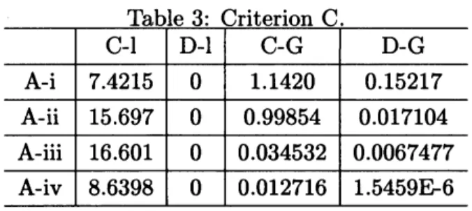
those in Sect. 2.

The result of the comparisons among the

models is shown in Table 3, where C-l denotes

the conventional logistic

curve

model 1 inSect.

2.1.1, D-l denotes the discrete logistic

curve

model of

Sect.

2.2,

C-G

denotes the

conven-tional Gompertz

curve

model 1 of Sect. 3.1.1,

and D-G denotes the discrete Gompertz

curve

model ofSect.

3.3.

The discrete logistic

curve

model matched all the four sets of the data.

This model reproduces the vaJues of the

pa-rameters of the exact solution when the exact

solution is used

as

the input data [30]. Thus,

the values of criterion $\mathrm{C}$ in this

case were

all

exactly

zero.

The conventional logistic

curve

model would be expected to provide

a

better fit

in termsof criterion $\mathrm{C}$ because each data set of

(A-i),

...,

(A-iv)

was

composed of exact

solu-tions ofthe logistic equation. However, for all

data sets of (A-i), $\ldots,$ (A-iv), the conventional

logistic

curve

model provided

a

poorer fit than

the conventional Gompertz

curve

model,

as

is

shown inTable 3.

We then used each model to estimate $k,$ the

initial fault content. The results of

compari-son

are shown in Table 4. The value of $k$

as

estimated by using the discrete logistic

curve

model matched the target value for all of the

four data sets. The estimates of $k$ provided

by the conventional logistic

curve

model

be-came more

accurate

as

the number of

avajl-able data points increased. Thus, in this case,

Table 3: Criterion C.

the estimate provided by using data set (A-i)

gave agood approximation to thetarget value.

Thediscrete and conventional Gompertz

curve

models,

on

the other hand,

were

much less

ac-curate than the discrete and conventional $1\mathrm{e}\succ$

gistic

curve

models. This

was

the

case

for all

four data sets. Given the

same

target value

of parameter $k,$ the first several values of

an

exact solution to the Gompertz equation

in-crease

faster than thoseofthe logistic equation.

Hence, estimates by the Gompertzmodels

were

much larger than the target value.

Table 4: Estimated parameter $k$

.

C-l D-l

C-G

D-G

A-i

99.23

100

88.11

200.0

A-ii 79.78 100 47.24 $1.175\mathrm{E}+6$

A-iii 72.17 100 $1.449\mathrm{E}+7$ $9.702\mathrm{E}+8$

A-iv 60.17 100 $1.198\mathrm{E}+84$ $1.855\mathrm{E}+184$

4.1.2 Data set $\mathrm{B}:$ The Gompertz

equa-tion

In this case,

we

used the

same

data sets, (B-i),

(B-ii), and (B-iii),

as

had been used in Sect. 3.

Comparative results forthe models

are

given

inTable5. ThediscreteGompertz

curve

model

matched all three data sets. The discrete

Gom-pertz

curve

model reproduces thevalues of the

parameters of

an

exact solution when that

ex-actsolution provides the input data [28]. Thus,

the corresponding values of criterion $\mathrm{C}$

were

all exactly

zero.

Table 5 shows that the

dis-crete and conventional logistic

curve

models

provided

a

poorer fit in terms of criterion $\mathrm{C}$

than did the discrete and conventional

Gom-pertz curve models. This was the case for each

data set in (B-i), $\ldots,$ (B-iii). This result is

rea-sonable because thedata setsarefromanexact

solution to the Gompertz equation.

Table 5: Criterion C. C-l D-l C-G D-G B-i 0.3346 0.014542.195E-4 0 C-l D-l C-G D-G B-i 0.3346 0.01454 2.195E-4 0 B-ii 1.141 0.01154 0.02100 0 B-iii

46.93

1.644E-32 0.2797

0

We used each model in estimating $k.$ The

comparative results

are

given in Table 6. The

values of $k$ estimated by the discrete

Gom-pertz

curve

model from all the three data sets

matched the target value. Estimates of $k$

provided by the conventional Gompertz

curve

model became

more

accurate

as

the number of

available data points increased. Thus, in this

case, the estimate provided by using data set

(B-i) gives

a

good approximation to the target

value. However, the discrete and conventional

logistic

curve

models

were

much less accurate

than the discrete and conventional Gompertz

curve

models. This

was

the

case

for all the

three data sets.

Table 6: Estimated parameter $k$

.

C-l D-l C-G D-G B-i 96.30 97.27 99.63

100

C-l D-l C-G D-G B-i 96.30 97.27 99.63

100

B-ii 31.44

55.36 78.16

100

B-iii

12.85 38.46 46.53

100

4.2

Evaluation

on

actual data

sets

4.2.1 Data set $\mathrm{C}$:Actual data set 1

We compared only the discrete logistic curve

model and the discrete Gompertz

curve

model

by using the

same

actual data set [30]

as was

used in Sect. 2, because both models yield

ac-curate parameter estimates in the

case

of data

that representexact solutions,

as

was

shown by

the previous comparisons.

Figure 5: Criterion value $\mathrm{v}\mathrm{s}.$ number of

avail-able data points.

We evaluatedthe parameterestimatae for

au

of the data and for only that data available

early in the test phase. We then used the

ae-timated parameters to calculate duae for

cri-terion C. As is shown in Fig. 5, the discrete

logistic

curve

model produced lower valuae for

$\mathrm{C}$ thanthe discrete Gompertz

curve

model

over

the whole test phase.

We estimated $k$

.

The comparative results

are

shown in Fig.

6.

The estimated values

are normalized on the total number of actual

software failurae. The discrete logistic

curve

model provided

more

accurate parameter

esti-mates. Moreover, this model providedaccurate

estimates throughout the rmge shown in the

figure.

Figure 6: Estimates ofparameter $k$

.

4.2.2Data

set

$\mathrm{D}$:Actual data set2

We used the same actual data set [14] as was

used in Sect. 3. As

was

shown in Sect. 3, the

discrete Gompertz

curve

model fit the actual

datavery well [28].

020 40 60

Avmlable data points$\mathrm{N}$

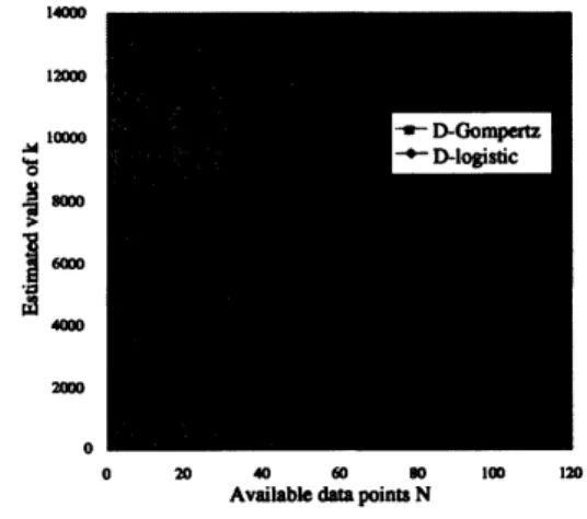
Figure 8: Estimates of parameter $k$

.

imitation. By introducing $F(t)= \frac{N(t)}{k},$ where

$F(t)$ is the fraction of potential adopters who

Figure 7: Criterion value $\mathrm{v}\mathrm{s}.$ number of avail- have adopted the product by time

$t,$ the Bass

able data points. _{model can be restated as}

We evaluated the parameter estimates for all the data and for only that the data available

early in the test phase. We then used the

es-timated parameters to calculate values for

cri-terion C. As is shown in Fig. 7, the discrete

Gompertz

curve

model produced lower values

for$\mathrm{C}$thanthe discrete logistic

curve

model

over

the whole test phase.

We usedeach modeltoestimate $k.$ The

com-parative results

are

shown in Fig.

8.

The

dis-crete Gompertz

curve

model providedthe

more

accurate parameter estimates. Moreover, this

model provided accurate parameter estimates

ffom quite early in the taet phase.

5

Bass model

5.1

Bass model and conventional

pa-rameter

estimations

Bass [1] suggaeted that the following

differen-tial equation

can

be used to represent the

dif-fusion process:

$\frac{dN(t)}{dt}=(p+\frac{q}{k}N(t))(k-N(t))$, (69)

where $N(t)$ is the cumulative number of

adopters at

a

time$t,$ $k$is theceiling,$p$isthe

co-efficient ofinnovation, and$q$isthecoefficient of

$\frac{dF(t)}{dt}=(p+qF(t))(1-F(t))$

.

₍₇₀₎

If$N(0)=0,$ simply integrating both sides of

equation (69) gives

us

the following

distribu-tion function to represent the time-dependent

aspect ofthe diffusion process:

$N(t)=k( \frac{1-e^{-(p+q)t}}{1+\mathrm{g}e^{-(p+q)t},p})$

.

(71)

Equation (71) yields the S-shaped diffusion

curve

captured by the Bass model.

A number of procedures for $\infty \mathrm{t}\mathrm{i}\mathrm{m}\mathrm{a}\mathrm{t}\mathrm{i}\mathrm{n}\mathrm{g}$ the

parameters$p,$ $q,$ $\mathrm{m}\mathrm{d}k$ of the Bass model have

been suggested. Mahajan et al. [11] compared

the performance of four $\mathrm{p}\mathrm{r}\mathrm{o}\mathrm{c}\mathrm{e}\mathrm{d}\mathrm{u}\mathrm{r}\mathrm{a}\mathrm{e}-\mathrm{t}\mathrm{h}\mathrm{e}$

ordi-nary

least squares (OLS) [1], maximum

like-lihood estimation (MLE) [32], nonlinear least

squarae (NLS) [33], and algebraic estimation

(AE) [10] $\mathrm{p}\mathrm{r}\mathrm{o}\mathrm{c}\mathrm{e}\mathrm{d}\mathrm{u}\mathrm{r}\mathrm{a}\mathrm{e}-\mathrm{o}\mathrm{n}$several sets of data.

They concluded that $\mathrm{N}\mathrm{L}\mathrm{S}$ yielded better

pre-dictionsaswell

as

more

valid estimates of

stan-dard

error

forthe parameter aetimates. Onthe

other hand, the

OLS

is the easiest to

imple-ment. Therefore,

we

$\mathrm{w}\mathrm{i}\mathrm{u}$ look at the OLS and

$\mathrm{N}\mathrm{L}\mathrm{S}$ procedurae in detail in the following two

sections.

5.1.1 Ordinary least squares procedure

The OLS procedure involves estimation of the

parameters by taking the discreteor regression

analogue of the differential equation (69). The

regression equation is given as

$X(i)=\alpha_{1}+\alpha_{2}N(ti-1)+\alpha_{3}N^{2}(t_{i-1})$, (72) where $X(i)$ $=$ $N(ti)-N(ti-1)$, (73) $\alpha_{1}$ $=$ $pk$, (74) $\alpha_{2}$ $=$ $q-p$, and (75) $\alpha_{3}$ $=$ $-q/k$. (76)

Given regression coefficients $\hat{\alpha}_{1},\hat{\alpha}_{2},$ and $\hat{\alpha}_{3}$,

theestimates of parameters$p,$ $q,$ and$k$

are

easy

to obtain: $\hat{p}$ _$=$ $\frac{-\hat{\alpha}_{2}+\sqrt{\hat{\alpha}_{2^{2}}-4\hat{\alpha}_{1}\hat{\alpha}_{3}}}{2}$ , (77) $\hat{q}$ $=$ $\frac{\hat{\alpha}_{2}+\sqrt{\hat{\alpha}_{2^{2}}-4\hat{\alpha}_{1}\hat{\alpha}_{3}}}{2},$ and (78) $\hat{k}$ $=$ $\frac{-\hat{\alpha}_{2}-\sqrt{\hat{\alpha}_{2^{2}}-4\hat{\alpha}_{1}\hat{\alpha}_{3}}}{2\hat{\alpha}_{3}}$

.

(79)

The main advantage of the OLS estimation

procedureis that it is easy to implement.

However, the$\mathrm{O}\mathrm{L}\mathrm{S}$procedurehas three

short-comings [32]. Firstly,

as

is clear ffomEq. (72),

in the presence of only

a

few data points and

the likely multicolinearityofvariables $(N(t_{\dot{\iota}-1})$

and $N^{2}(t_{\dot{\iota}-1})),$

one

may obtain parameter

esti-mates that

are

unstable

or

possess wrongsigns

(examples [4, 32, 33]). Secondly, the standard

errors

of the estimates

are

not available since

parameters $p,$$q,$ and $k$

are

nonlinearfunctions

of $\alpha_{1},\alpha_{2},$ and $\alpha_{3}$

.

The

error

term, however,

does contain the net effect of

au

sources

of

er-$\mathrm{r}\mathrm{o}\mathrm{r}.$ Thirdly, the derivative of $N(t)$ which is

obtained at $t:-1$ by the right-hand side of Eq.

(73) will always be overestimated for time

in-tervalsbefore the point of inflection and

under-estimated after that. That is,

a

time-interval bias is present in the

OLS

approach since dis-crete time-series data

are

used to aetimate $\mathrm{a}$

continuous-time model.

$1\hat{\alpha}_{1}>0,\hat{\alpha}_{2}>0$, and$\hat{\alpha}_{3}<0$because$\hat{p},\hat{q}$,and

$\hat{k}$are positive.

5.1.2 Nonlinear least squares

estima-tion

The nonlinear least squares estimation

proce-dure suggested by Srinivasan and Mason [33]

was designed to

overcome some

of the

short-comings of $\mathrm{M}\mathrm{L}\mathrm{E}$ procedure [32], which itself

was

designed to

overcome

the shortcomings of

the

OLS

procedureof Schmittlein andMahajan

[32]. Fromthe cumulativedistributionfunction

given by

$F(t)= \frac{1-e^{-bt}}{1+ae^{-u}}$, (80)

Srinivasan

and Mason suggest that parameter

estimates $\hat{p},\hat{q},$ and

$\hat{k}$

can

be obtained by

us-$\mathrm{i}\mathrm{n}\mathrm{g}$the following expression for the number of

adopters$X(i)$ inthe $i\mathrm{t}\mathrm{h}$ timeinterval $(t:-1,t:)$:

$X(i)=k(F(t_{\dot{l}})-F(t:-1))+\mu:$, (81)

where _Pi is

an

additive

error

term. Based

on

Eq. (81), parameters $p,q,$ and $k$ and their

asymptotic standard

errors can

be directly

ae-timated.

The $\mathrm{N}\mathrm{L}\mathrm{S}$ procedure

overcomes

the

time-intervaJ bias present in the $\mathrm{O}\mathrm{L}\mathrm{S}$ procedure.

Furthermore, since the

error

term may be

con-sidered to represent the net effect of sampling

errors, excluded variables (such

as

economic

conditions and marketing mix variables), and

$\mathrm{m}\mathrm{i}\mathrm{s}$-specification of the density function, the

derived standard

errors

for the parameter

ae-timates may be

more

realistic. However, since

the$\mathrm{N}\mathrm{L}\mathrm{S}$procedure employs various search

rou-tines in estimating the parameters, parameter

estimates may sometimes be very slow to

con-verge

or

may not converge, the final estimates

may be sensitive to the initial dues for $p,q$,

and $k$,

or

the procedure may provide

a

non-global optimum.

5.2

Discrete Bass model

We propose

a

discrete Bass model, which is $\mathrm{a}$

form of

a

discrete Riccati equation [5]. The dis-crete Bass model enables

us

toforecast the

dif-fusion innovation without using

a

continuous-time Bass model, because the discrete model

has

an

exact solution.

The discrete Bass model is described

as

fol-lows:

$\frac{N_{n+1}-N_{n-1}}{2\delta}$

$=p(k- \frac{N_{n+1}+N_{n-1}}{2})$

14

$( \frac{k}{2}(N_{n+1}+N_{n-1})-N_{n+1}N_{n-1})$

.

(82)

The exact solution to equation (82) is written

as

$N_{n}=k( \frac{1-(\frac{1-\delta(q+p)}{1+\delta(q+p)})^{\frac{n}{2}}}{1+p\mathrm{f}\mathrm{l}(\frac{1-\delta(q+p)}{1+\delta(q+p)})^{\frac{n}{2}}})$, (83)

where $n=7t.$ This equation has also appeared

in work

on

SRGM [37].

Applying $\mathrm{O}\mathrm{L}\mathrm{S}$ to the discrete Bass model

is easy because the model is basically

a

time-discrete equation. The $\mathrm{O}\mathrm{L}\mathrm{S}$ procedure is the

simplest method of parameter estimation for

the discrete Bass model. In the continuous

Bass model, the forward difference equation,

which acts

as

aregression equation inthe $\mathrm{O}\mathrm{L}\mathrm{S}$

procedure, is

an

approximation of the

differ-ential equation. However, in the discrete Bass

model, themodel itselfis directly applied

as

the

regression equation. Moreover,

a

solution of

the discrete Bassmodel providesthe

same

val-$\mathrm{u}\mathrm{e}\mathrm{s}$

as

asolution of the continuous Bass model

through the following equations:

$p_{d}=\kappa p$, (84) $q_{d}=\kappa q$, (85)

$\kappa=\frac{1}{\delta(\mathrm{p}+q)}(\frac{1-\exp(-2(q+p))}{1+\exp(-2(q+p))})$ , (86)

where $p_{d}$ and $q_{d}$

mean

$p$ and $q$ in Eq. (83),

respectively.

Wepropose two regression models. The first

is the following equation:

$S_{n}=2(a+b(N_{n+1}+N_{n-1})+cN_{n+1}N_{n-1})+\epsilon(n)$, (87) where $S_{n}=N_{n+1}-N_{n-1}$, (88) $a=kp$, (89) $b=\mathrm{L}^{-}A2$ ’ (90) $c=-k\mathrm{A}$, (91)

$\epsilon(n)$ : error, and $E[\epsilon(n)]=0$

.

(92)

Given regression

coefficients2

$a,$ $b$, and $c$,

pa-rameter estimates $\hat{p},\hat{q},$ and $\hat{k}$

are

easily

ob-tained as follows:

$\hat{p}$ _$=$ $-b+\sqrt{b^{2}-ac}$, (93) $\hat{q}$ _$=$ $b+\sqrt{b^{2}-ac},$ and (94) $\hat{k}$

$=$ $\frac{-b-\sqrt{b^{2}-ac}}{c}$

.

(95)

The other regression model is the following

equation: $M_{n}=A+BN_{n-1}+C(N_{n+1}-N_{n-1})+\epsilon(n)$, (96) where $M_{n}=N_{n+1}N_{n-1}$, (97) $A=\underline{k}_{f,q}^{2}$, (98) $B= \frac{k(q-p)}{q}$, (99) $C= \frac{k(q-p-1)}{2q}$, (100)

$\epsilon(n)$ : error, and $E[\epsilon(n)]=0$

.

(101)

Given regression$\mathrm{c}\mathrm{o}\mathrm{e}\mathrm{f}\mathrm{f}\mathrm{i}\mathrm{c}\mathrm{i}\mathrm{e}\mathrm{n}\mathrm{t}\mathrm{s}^{3}A,$$B$

,

and $C$

,

pa-rameter estimates $\hat{p},\hat{q},$ and $\hat{k}$

are

easily $\mathrm{o}\mathrm{k}$

tained

as

follows:

$\hat{p}$ $=$ $\frac{-B+\sqrt{B^{2}+4A}}{2B-C}$, (102) $\hat{q}$ $=$ $\frac{B+\sqrt{B^{2}+4A}}{2B-C},$ and (103) $\hat{k}$

$=$ $\frac{B+\sqrt{B^{2}+4A}}{2}$

.

(104)

These procedures have the advantage of

sim-plicity, which is also provided by parameter

estimation through the

OLS

procedure in the

continuous Bass model.

Applying the $\mathrm{N}\mathrm{L}\mathrm{S}$procedure to the discrete

Bass model is also relatively easy, because the

discrete Bass model has

an

exact solution (83).

We propose two $\mathrm{N}\mathrm{L}\mathrm{S}$ procedures for the

dis-crete Bass model. One of these providae

esti-mated parameter $\hat{p},\hat{q},$ $\mathrm{m}\mathrm{d}\hat{k}$ by using the

fol-lowing expressions for the number ofadopters

$X_{n}$ in the $n\mathrm{t}\mathrm{h}$ time intervaJ:

$X_{\hslash}=N_{n+1}-N_{n-1}+\mu_{\hslash}$, (105) $2a>0,$ $b>0$, and $c<\mathrm{O}$ because$\hat{p},\hat{q}$, and $\hat{k}$ are poeitive.

$3A>0,$ $B>0,$ and$C<\mathrm{O}$ because$\hat{p},\hat{q},$ and

$\hat{k}$ are poeitive.

where $\mu_{n}$ is

an

additive

error

term.

The other $\mathrm{N}\mathrm{L}\mathrm{S}$ procedure for the discrete

Bass model is the following equation:

$\mathrm{Y}_{n}=N_{n+1}N_{n}+\nu_{n}$ (106)

where $\mathrm{Y}_{n}$ is the ratio between the number of

adopters at the $n\mathrm{t}\mathrm{h}$ time-step and that at the

$(n+1)\mathrm{s}\mathrm{t}$ time-step.

These procedures have the advantage of

al-lowing the direct estimation of the

asymp-totic standarderrorsof theparameters,

as

does

the $\mathrm{N}\mathrm{L}\mathrm{S}$ procedure with the continuous Bass

model. Moreover, since the

error

termsinthese

procedures may be considered to represent the

net effect of sampling errors, excluded

vari-ables, andmis-specificationof thedensity

func-tion,thederived standard

errors

for the

param-eter estimatesmay be

as

realistic

as

those ofthe

$\mathrm{N}\mathrm{L}\mathrm{S}$procedure for the continuous Bass model.

Either of the$\mathrm{O}\mathrm{L}\mathrm{S}$procedures in the discrete

Bass model

overcomes

the three shortcomings

of the $\mathrm{O}\mathrm{L}\mathrm{S}$ procedure in the continuous Bass

model: the time-interval bias, standard error,

and multicolinearity.

When

we use

the discrete Bass model to

avoid using thecontinuousmodelin forecasting

the diffusion of innovation, there is

no

time-interval bias because the model is

a

discrete

model. Ehrthermore,

even

ifthe discrete Bass

model is regarded

as

only the procedure used

to obtain the parameters for the continuous

model, the $\mathrm{O}\mathrm{L}\mathrm{S}$ procedures do not suffer ffom

a

time-interval bias because

a

solution of the

discrete Bass model gives the

same

values

as a

solution of the continuous Bass model,

as

was

already stated in this section.

$\mathrm{R}\mathrm{o}\mathrm{m}$ Eq. (82), Eq. (87) is equivalent to Eq.

(105), and Eq. (96) is equivalent to Eq. (106)

under

no

constraints. Therefore, the

same

pa-rameter estimation is done through both

Pro-cedures in the discrete Bass model. This is

a

significant advantageof the discrete Bass model

because

we can

getthe global optimum through

$\mathrm{O}\mathrm{L}\mathrm{S},$ and then apply $\mathrm{N}\mathrm{L}\mathrm{S}$to obtain the

stm-dard

error.

By using both procedures together,

we

overcome

their shortcomings in separate

ap-plication. That is, thestandarderror of the

re-sults of the OLS procedureis obtained through

the $\mathrm{N}\mathrm{L}\mathrm{S}$ procedure. Equations (87) and (96)

overcome

the three shortcomings of$\mathrm{N}\mathrm{L}\mathrm{S}:$ that

final parameter estimates

are

sensitive to the

initial values of$p,q$, and$k$, that parameter

esti-mates may sometimes beveryslow toconverge

or

may not converge at all, and that the

op-timum provided by the procedure may not be

global.

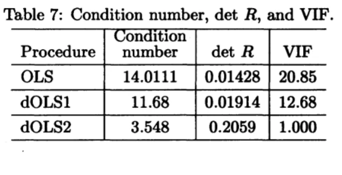
Table 7 shows the condition number, the

de-terminant ofcorrelation matrix$R,$and the

vari-ance

inflation factors (VIFs) for three

proce-dures: the conventional $\mathrm{O}\mathrm{L}\mathrm{S}$procedure (OLS),

discrete analogue 1 of the $\mathrm{O}\mathrm{L}\mathrm{S}(87)$ (dOLSl),

and discreteanalog2 oftheOLS (96) $(\mathrm{d}\mathrm{O}\mathrm{L}\mathrm{S}2)$,

where

we

chose the exact solution $(p=0.002$,

$q=1,$ $m=100)$ to differential equation (69)

as

the data from every period ffom $t=0$ to

$t=11.$ The $\mathrm{V}\mathrm{F}$ in the conventional

OLS row

is the VIF of the variable $N(t_{\dot{*}-1})$ in Eq. (72).

$\mathrm{R}\mathrm{o}\mathrm{m}$ the definition of the $\mathrm{V}\mathrm{F},$ the value of

the $\mathrm{V}\mathrm{F}$ of the variable $N(t:-1)$ is the

same as

that of the $\mathrm{V}\mathrm{I}\mathrm{F}$ of the other variable, $N(t:)^{2}$

.

The $\mathrm{V}\mathrm{I}\mathrm{F}$ in the dOLSl

row

is the VIF of the

variable $(N_{n+1}+N_{n-1});$ the $\mathrm{V}\mathrm{I}\mathrm{F}$inthe $\mathrm{d}\mathrm{O}\mathrm{L}\mathrm{S}2$

row is the $\mathrm{V}\mathrm{F}$ of the variables _{$N_{n-1}$} in Table

7. $\mathrm{d}\mathrm{O}\mathrm{L}\mathrm{S}2$ excludes the problem of

multicolin-earity. Therefore, with this procedure, awrong

signfor

a

parametersuggests that the obtained

data is not appropriate for the Bass model.

Table 7: Condition number, $\det R$, and VIF.

on

ltl0n

Procedure number $\det R$ $\mathrm{V}\mathrm{I}\mathrm{F}$

Procedure number

on

ltlon $\det$ $R$ VIF

$\mathrm{O}\mathrm{L}\mathrm{S}$

14.0111

0.01428 20.85

dOLSl 11.68

0.01914

12.68

$\mathrm{d}\mathrm{O}\mathrm{L}\mathrm{S}2$ 3.548 0.2059 1.000

5.3Parameter estimation

The accuracy of the parameter aetimate pro-vided by the conventional

OLS

procedure $\mathrm{m}\mathrm{d}$

the two OLS procedures in the discrete Bass

model

was

compared. Tocomparetheaccuracy

of the parameter estimatesonly,

we

choee data

which satisfy theexact solution $(p=0.002,$$q=$

$1,$$k=100)$ ofdifferential equation (69) in

ev-$\mathrm{e}\mathrm{r}\mathrm{y}$ periodffom $t=0$to$t=11$ (the

same

data

as was

usedinthe previous section). Thisdata

has apoint of inflection where $t^{*}=6.2022$ and

$N(t^{*})=49.9$

.

We analyzed three sets of data;

data 1: the data up to the point just before

the point of inflection $(t=0,1, \cdots, 6),$ data 2:

the data _uP to the pointjust after the point of

inflection $(t=0,1, \cdots, 7)$,and data3:thedata

up tothe ceiling $(t=0,1, \cdots, 11)$

.

The resultsofcomparisonofthe conventional

OLS, dOLSl and $\mathrm{d}\mathrm{O}\mathrm{L}\mathrm{S}2$procedures

are

given

in Table 8. Both dOLSl and $\mathrm{d}\mathrm{O}\mathrm{L}\mathrm{S}2$ provide

accurate estimates. Since

we

used the exact

solution to provide the data,

an

accurate

pro-cedure should reproduce the values of the

pa-rameters of the exact solution. Table

8

shows

that bothdOLSland$\mathrm{d}\mathrm{O}\mathrm{L}\mathrm{S}2$reproduced _$k$

per-fectly,

even

when the data did not include the

point of inflection and there

were

fewer than

eight data points.

Table 8: Estimatedparameter $k$

.

Data set OLS dOLSl $\mathrm{d}\mathrm{O}\mathrm{L}\mathrm{S}2$

Data set OLS dOLSl $\mathrm{d}\mathrm{O}\mathrm{L}\mathrm{S}2$

data 1 55.71

100

100

data 2 71.61 100 100

data 3 97.27

100

100

The accuracy of the conventional $\mathrm{O}\mathrm{L}\mathrm{S}$

$\mathrm{p}\mathrm{r}\sim$

cedure is poor daepite the fact that the data

is drawn ffom

an

exact solution of the

differ-ential equation. In particular, the conventional

OLS procedureyields poorestimates of the

pa-rameters with data 1. This is consistent with

the findingsof Heeler and Hustad [4] and

Srini-vasan

andMason [33]. Through empirical

stud-$\mathrm{i}\mathrm{e}\mathrm{s}$,they found thatstableandrobust estimates

of the parameters of the basic diffusion $\mathrm{m}\mathrm{o}\mathrm{d}-$

$\mathrm{e}\mathrm{l}\mathrm{s}$ cannot be obtained unless

one

uses

at least

eight data points, within which the point of

inflection falls. The estimates of parameters

with data 2

were

$\mathrm{a}\mathrm{k}\mathrm{o}$not accurateenough,

even

though data 2satisfies the above condition.

Whenever adata set is aset from

an

exact

solution of Eq. (69), the dOLSl and $\mathrm{d}\mathrm{O}\mathrm{L}\mathrm{S}2$

procedures reproduce all values of the

param-eters, $\mathrm{i}.\mathrm{e}.,$ $k,$

$p$, and $q;$ theoretically, this is

because the solution ofEq. (82) is the

same

as

that of Eq. (69) through $\mathrm{E}\mathrm{q}\mathrm{s}$

.

(84), (85),

and (86). This is independent of the number of

data points and the values of the parameters.

However, the conventional$\mathrm{O}\mathrm{L}\mathrm{S}$proceduredoes

not reproduce values of the parameters and de

pends

on

the number of data points,

as

shown

in Table 8, because regression Eq. (72) does

not have

an

exact solution and gives only

an

approximation ofthe Bass model.

We also evaluated the discrete Bass model

on

actual data. This data

was

the

same as

that used by Mahajan etal. [11], which

was on

the data diffusion of

seven

products:

room

air

conditioners, color televisions, clothes dryers,

ultrasound, mammography, foreign language,

and accelerated

program.

These

seven

prod-ucts represent

a

diverse set of innovations, and

thusof sets ofdata, for all of which

a

minimum

ofeight annual data points covering the peak

(point of inflection), is available. In addition,

these products have been used extensively in the diffusion modeling literature to illustrate

the application of alternative diffusion models

or

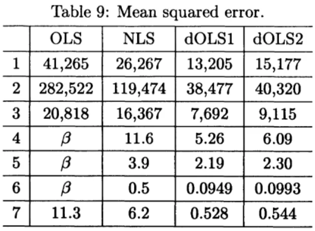
estimation procedures [1, 9, 32, 33].

To compare the predictive performance of

the four estimation procedures, the OLS and the $\mathrm{N}\mathrm{L}\mathrm{S}$ procedure in the continuous Bass

model and the two

OLS

procedures in the

dis-creteBass model, resultsrelatedto

a

statisticof

fit (MSE)

are

given inRble

9.

The numbers(1,

2, $\cdots,$ $7$) in the left column repraeent,

raepec-tively,

room

air conditioners, color televisions,

clothesdryers, ultrasound, mammography,

for-eign language, and accelerated program. The

statistics of fit for $\mathrm{d}\mathrm{O}\mathrm{L}\mathrm{S}2$ is not directly

com-parable with thoseofthe other estimation$\mathrm{p}\mathrm{r}(\succ$

cedures, because the

error

term of $\mathrm{d}\mathrm{O}\mathrm{L}\mathrm{S}2$ is

different from the error terms ofthe other

es-timation procedures. However, from $\mathrm{E}\mathrm{q}\mathrm{s}$

.

(87)

and (96), the

error

term $\epsilon(n)$ maybe regarded

as

following

$\epsilon(n)=\frac{k}{q}\epsilon(n)$

.

(107)

Therefore,

we

compared the fit statistics of

$\mathrm{d}\mathrm{O}\mathrm{L}\mathrm{S}2$ with those of other procedures by

us-$\mathrm{i}\mathrm{n}\mathrm{g}$this equation.

Ofthefourprocedures (the OLS, $\mathrm{M}\mathrm{L}\mathrm{E},$$\mathrm{N}\mathrm{L}\mathrm{S}$,

and $\mathrm{A}\mathrm{E}$ procedures in the continuous Bass

model), the $\mathrm{N}\mathrm{L}\mathrm{S}$ procedure provides the best

fit to the data [11]. Mahajan et al. stated

that, if

we assume

global optimum parameter

Table 9: Mean squared

error.

$\mathrm{O}\mathrm{L}\mathrm{S}$ $\mathrm{N}\mathrm{L}\mathrm{S}$ dOLSl $\mathrm{d}\mathrm{O}\mathrm{L}\mathrm{S}2$

OLS NLS dOLSl $\mathrm{d}\mathrm{O}\mathrm{L}\mathrm{S}2$

1 41,265 26,267 13,205 15,177 2 282,522 119,474 38,477 40,320 3 20,818 16,367 7,692 9,115 4 $\beta$ 11.6 5.26 6.09 5 $\beta$ 3.9 2.19

2.30

6 $\beta$ 0.5 0.0949 0.0993 7

11.3

6.2

0.528

0.544

OLS $\mathrm{N}\mathrm{L}\mathrm{S}$ dOLSl $\mathrm{d}\mathrm{O}\mathrm{L}\mathrm{S}2$

1 0.0170

0.0094

0.0139

0.0107

2 0.0357 0.0185

0.02448

0.02194

3

0.0196 0.0136

0.01790

0.014322

4 $\beta$

0.0013 -0.01755

-0.02826

5 $\beta$

0.0004 -0.02501

-0.030308

6 $\beta$

0.0019

-0.0249

-0.02871

7

0.0120 0.0007 -0.01825

-0.0215363

estimates, the $\mathrm{N}\mathrm{L}\mathrm{S}$ procedure should, by

defi-nition, provide the best fit in terms of the

mean

squared

error

[11]. However,

a

comparison of

the statistics of fit in Table 9 indicates that

both dOLSl and $\mathrm{d}\mathrm{O}\mathrm{L}\mathrm{S}2$ provided

a

better fit

tothe data than did the$\mathrm{O}\mathrm{L}\mathrm{S}$or$\mathrm{N}\mathrm{L}\mathrm{S}$interms of

mean

squared

error.

Thefit statistic ofdOLSl

was

the best of all. A $\beta$ in Table 9 indicates

cases

where the $\mathrm{O}\mathrm{L}\mathrm{S}$ procedure yielded an

in-correct sign for the regression coefficient $\hat{\alpha}_{1}$ in

the regression equation.

Table 10: Parameter estimates of$k$

.

$\mathrm{O}\mathrm{L}\mathrm{S}$ $\mathrm{N}\mathrm{L}\mathrm{S}$ dOLSl $\mathrm{d}\mathrm{O}\mathrm{L}\mathrm{S}2$ $1$ $17.1\mathrm{E}6$ $18.7\mathrm{E}6$ $18.0\mathrm{E}6$ $17.1\mathrm{E}6$

$2$ $35.5\mathrm{E}6$

.

$39.7\mathrm{E}6$ $39.1\mathrm{E}6$ $38.4\mathrm{E}6$ $3$ $15.3\mathrm{E}6$ $16.5\mathrm{E}6$ $16.19\mathrm{E}6$ $15.3\mathrm{E}6$

OLS $\mathrm{N}\mathrm{L}\mathrm{S}$ dOLSl $\mathrm{d}\mathrm{O}\mathrm{L}\mathrm{S}2$

1 $17.1\mathrm{E}6$ $18.7\mathrm{E}6$ $18.0\mathrm{E}6$ $17.1\mathrm{E}6$

2 $35.5\mathrm{E}6$

.

$39.7\mathrm{E}6$ $39.1\mathrm{E}6$ $38.4\mathrm{E}6$

3 $15.3\mathrm{E}6$ $16.5\mathrm{E}6$ $16.19\mathrm{E}6$ $15.3\mathrm{E}6$

4 $\beta$ 167.4 187.2 180.2

5 $\beta$ 111.4 122.1 121.2

6 $\beta$

37.6

40.1

39.6

7

63.6

64.4

65.5

65.1

Tables 10 and 11 show the parameters

esti-mated by the OLS, $\mathrm{N}\mathrm{L}\mathrm{S},$ dOLSl, $\mathrm{m}\mathrm{d}\mathrm{d}\mathrm{O}\mathrm{L}\mathrm{S}2$

procedures. Again, $\beta$ indicates where the

OLS

procedure yielded

an

incorrect sign for the

re-gression coefficient $\hat{\alpha}_{1}$ in the regression

equa-tion. The results for the parameter estimates

in Table 11 show that bothdOLSl and $\mathrm{d}\mathrm{O}\mathrm{L}\mathrm{S}2$

providedthewrongsignforthe regression

coef-ficient$a$in Eq. (87) andforthe regression

coef-ficient $A$ in Eq. (96) forultrasound,

mammog-raphy, foreign language, and accelerated $\mathrm{p}\mathrm{r}x$

gram. Both $a$ in Eq. (87) and $A$ in Eq. (96)

are

the regression coefficients of the constant

term.

Table 11: Parameter estimates of$p$

.

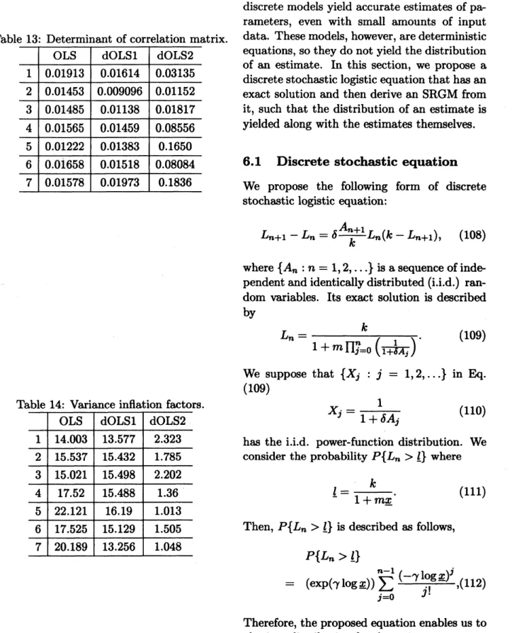
A wrong sign in Table 11, however, doesnot

indicate multicolinearity. Tables 12, 13, and

14, respectively, show the condition number,

determinantof the correlationmatrix, and

vari-ance

inflation factors for each product. These tables show that there is

no

multicolinearity in $\mathrm{d}\mathrm{O}\mathrm{L}\mathrm{S}2.$ Cases where the wrong signs

were

applied havesmaller condition numbers, larger

determinants of the correlation matrices, and

smaller VIFs than the

cases

that had the right

signs. Therefore, the wrong sign

on a

parame-$\mathrm{t}\mathrm{e}\mathrm{r}$ suggests that the obtained data is not

ap-propriate for the Bass model.

Table 12: Condition number. OLS dOLSl $\mathrm{d}\mathrm{O}\mathrm{L}\mathrm{S}2$

1 11.943 12.615 7.743

2 13.321 15.768 10.123 3

13.145

14.499

9.723

OLS dOLSl $\mathrm{d}\mathrm{O}\mathrm{L}\mathrm{S}2$

1 11.943 12.615 7.743 2 13.321 15.768 10.123 3

13.145

14.499

9.723 4

13.380

13.436 4.513 5 14.982 13.648 3.703 6 13.132 13.213 4.700 7 13.546 11.736

3.503

131

6

$\mathrm{D}_{\acute{1}}\mathrm{s}\mathrm{c}\mathrm{r}\mathrm{e}\mathrm{t}\mathrm{e}$

stochastic logistic

curve

model

Table 13: Determinant of correlation matrix.

OLS dOLSl $\mathrm{d}\mathrm{O}\mathrm{L}\mathrm{S}2$

1

0.01913

0.01614

0.03135

2 0.01453

0.009096 0.01152

3

0.01485

0.01138

0.01817

OLS dOLSl $\mathrm{d}\mathrm{O}\mathrm{L}\mathrm{S}2$

1

0.01913

0.01614

0.03135

2 0.01453

0.009096 0.01152

3

0.01485

0.01138

0.01817

4

0.01565

0.01459

0.08556

5 0.01222

0.01383

0.1650 6

0.01658

0.01518

0.08084

7 0.01578

0.01973

0.1836

Asshown intheprevious sections, theproposed

discrete models yield accurate estimates ofpa

rameters,

even

with small amounts of input

data. These models, however,

are

deterministic

equations, sotheydo not yield the distribution

of

an

estimate. In this section,

we

propose $\mathrm{a}$

discretestochasticlogistic equation that has

an

exact solution and then derive

an

SRGM

from

it, such that the distribution of

an

estimate is yielded along withthe estimates themselves.

6.1

Discrete

stochastic equation

We propose the following form of discrete

stochastic logistic equation:

$L_{n+1}-L_{n}= \delta\frac{A_{n+1}}{k}L_{n}(k-L_{n+1})$, (108)

Table 14: Variance inflation factors.

OLS

dOLSl $\mathrm{d}\mathrm{O}\mathrm{L}\mathrm{S}2$

where $\{A_{n} : n=1,2, \ldots\}$is

a

sequence of

inde-pendentand identically distributed (i.i.d.)

ran-$\mathrm{d}\mathrm{o}\mathrm{m}$ variables. Its exact solution is daecribed

by

$L_{n}= \frac{k}{1+m\prod_{j=0}^{n}(\frac{1}{1+\delta A_{\mathrm{j}}})}$

.

(109)

We suppose that $\{Xj : j=1,2, \ldots\}$ in Eq.

(109)

$X_{j}= \frac{1}{1+\delta A_{j}}$ (110)

$\mathrm{O}\mathrm{L}\mathrm{S}$ dOLSl $\mathrm{d}\mathrm{O}\mathrm{L}\mathrm{S}2$

1

14.003

13.577

2.323

2 15.537 15.432 1.785

3

15.021

15.498

2.202

4 17.52 15.488

1.36

5 22.121 16.19

1.013

6

17.525

15.129 1.505 7 20.189 13.256

1.048

has the i.i.d. power-function distribution. We

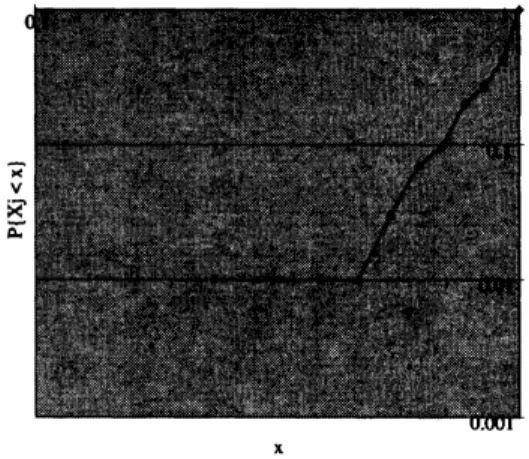
consider the probability $P\{L_{n}>\underline{l}\}$ where

$\underline{l}=\frac{k}{1+m\underline{x}}$

.

(111)

Then, $P\{L_{n}>\underline{l}\}$ is described

as

follows,

$P\{L_{n}>\underline{l}\}$

$=$ $( \exp(\gamma\log\underline{x}))\sum_{j=0}^{n-1}\frac{(-\gamma 1\mathrm{o}\mathrm{g}\underline{x})^{j}}{j!},(112)$

Therefore, the proposed equationenables

us

to

obtain

a

distribution for the estimate at

a

step

$n$

.