非平滑凸最適化に関する並列計算手法 (非線形解析学と凸解析学の研究)

(1)

非平滑凸最適化に関する並列計算手法

Parallel

Computing

Method for Nonsmooth

Convex

optimization

明治大学理工学部情報科学科菱沼和弘，飯塚秀明

Kazuhiro HISHINUMA and Hideaki IIDUKA

Department ofComputer Science, School of Science and Technology,

Meiji University

ABSTRACT. Inthis paper, weconsider the problem of minimizing thesum of

nondiﬀeren-tiable, convex functionsover aclosed convex set in a real Hilbert space, which is simple in

thesensethat the projectiononto it canbe easilycalculated. We presentaparallel subgra-dient methodfor solving it and the two convergence analyses of the method. One analysis shows that the parallel method withasmall constant step size approximates asolution to

theproblem. The other analysis indicates that the parallel method withadiminishing step

size convergestoasolution tothe problem in thesense of the weak topology of the Hilbert space. Finally, we numerically compare our method with the existing method and state future workonparallelsubgradient methods.

1. INTRODUCTION

This paper considers the following standard nonsmooth convex minimizationproblem.

Problem 1.1. Let $f_{i}(i=1,2, \ldots, K)$ be convex, continuous functionals on a real Hilbert

space $H$ and let $C$ be a nonempty, closed convex_{subset of} $H$. Then,

minimize $\sum_{i=1}^{K}f_{i}(x)$ subject to$x\in C.$

A useful algorithm for solving Problem 1.1 is the incremental subgradient method [9, 12], and it is defined as follows: for defining $P_{C}$ as the projection onto $C$ and $\partial f_{i}(x)$ as the

subdiﬀerential of$f_{i}$ at $x\in H$ $(i=1,2, \ldots , K)$, an iteration $(n+1)$ of the algorithm is

(1.1) $\{\begin{array}{l}\psi_{0,n}:=x_{n},\psi_{i,n}:=P_{C}(\psi_{i-1,n}-\lambda_{n}g_{i,n}) , g_{i,n}\in\partial f_{i}(\psi_{i-1,n})(i=1,2, \ldots, K) ,x_{n+1}:=\psi_{K,n}.\end{array}$

Algorithm (1.1) requires us to use $P_{C}$ each iteration. Hence, we assume that $C$ is simple in

thesensethat $P_{C}$ can beeasily calculatedwithin afinitenumber ofarithmetic operations [1,

p.406], [2, Subchapter 28.3]. Some incremental methods that can be applied when $C$ is not

always simple werepresented in [4, 6, 7].

Meanwhile, parallel proximal algorithms [2, Proposition 27.8], [3, Algorithm 10.27], [10] are

(2)

convex $f_{i}$ which maps every $x\in H$ to the uniqueminimizer of$f_{i}+(1/2)\Vert x-\cdot\Vert^{2}$, where $\Vert\cdot\Vert$

stands for the norm of $H$. The parallel gradient algorithms presented in [6, 7] work only

when $f_{i}$ is diﬀerentiable and convex, and $C$ is not always simple.

This paper presents

a

parallel subgradient method for solving Problem 1.1. The proposed method doesnot useany proximityoperators, in contrast to the algorithms in [2, Proposition

27.8], [3, Algorithm 10.27], [10]. Next, we present convergence analyses for the two step-size

rules: a constant step-size rule and a diminishing step-size rule. We show that the proposed method withasmallconstantstepsizeapproximatesasolution to Problem 1.1. We also show that the algorithm with a diminishing step size weakly converges to a solution to Problem 1.1.

This paper is organized

as

follows. Section 2givesthemathematicalpreliminaries. Section

3presents theparallel algorithm for minimizingthesumofconvexfunctionals over a simple,

convex closed constraint set and studies its convergence properties for a constant step size andadiminishing step size. Section4 providesnumericalexamples of the algorithm. Section 5 concludes the paper and mentions future work on parallel subgradient methods.

2. PRELIMINARIES

Let $H$ be areal Hilbert space with inner product and its induced norm $\Vert$ . Let $\mathbb{N}$

denote the set of all positive integers includingzero.

2.1. Subdiﬀerentiability and projection. The

_{subdiﬀerential}

[2, Definition 16.1], [11,

Section 23], [13, p.132] of $f:Harrow \mathbb{R}$ is the set-valued operator,

$\partial f:Harrow 2^{H}:x\mapsto\{u\in H:f(y)\geq f(x)+\langle y-x, u\rangle(y\in H)\}.$

Suppose that $f:Harrow \mathbb{R}$iscontinuous andconvexwith$dom(f)$ $:=\{x\in H:f(x)<\infty\}=H.$

Then, $\partial f(x)\neq\emptyset(x\in H)$ [$2_{\}}$ Proposition 16.14(ii)]:

Proposition 2.1. [2, Proposition 16.17] Let $f:Harrow \mathbb{R}$ be continuous and convex with

$dom(f)=H$. Then, thefollowing are equivalent:

(i) $f$ is bounded

on every

bounded subset

of

$H.$

(ii) $f$ is Lipschitz continuous relative to every bounded subset

of

$H.$

(iii) $dom(\partial f)$ $:=\{x\in H:\partial f(x)\neq\emptyset\}=H$ and $\partial f$ maps every bounded subset

of

$H$ to a

bounded set.

The metric projection [2, Subchapter 4.2, Chapter 28] onto a nonempty, closed convex set

$C(\subset H)$ is denoted by $P_{C}$. It is defined by _{$P_{C}(x)\in C$} and $\Vert x-P_{C}(x)\Vert=\inf_{y\in C}\Vert x-y\Vert$

$(x\in H)$

.

$P_{C}$ is (firmly) nonexpansive with Fix$(P_{C}):=\{x\in H:P_{C}(x)=x\}=C[2,$

Proposition 4.8, (4.8)].

2.2. Main problem. This paper deals witha networked system with $K$users. Throughout

this paper, we assume the following.

Assumption 2.2.

(3)

(A2) $f_{i}:Harrow \mathbb{R}(i=1,2, \ldots, K)$ iscontinuous and convexwith$dom(f_{i})=dom(\partial f_{i})=H,$

and $\cup\{\partial f_{i}(x):x\in B\}$ is bounded for a bounded set $B(\subset H)$;

(A3) User $i(i=1,2, \ldots, K)$ _can

use

$P_{C}$ and $\partial f_{i}$;

(A4) User $i(i=1,2, \ldots, K)$ _can _{communicate with all} _users.

The main objective ofthis paper is to solve the following problem.

Problem 2.3. Under Assumption 2.2, find a minimizer of $\sum_{x’=1}^{K}f_{i}$ over $C.$

3. PARALLEL ALGORITHM

We present a parallel algorithm for solving Problem 2.3.

Algorithm 3.1.

Step O. All users set $x_{0}\in H$ arbitrarily and $\{\lambda_{n}\}\subset(0, \infty)$.

Step 1. User $i(i=1,2, \ldots, K)$ computes $y_{i,n}\in H$ as follows:

$\{\begin{array}{l}g_{i,n}\in\partial f_{i}(x_{n}) ,y_{i,n}:=P_{C}(x_{n}-\lambda_{n}g_{i,n}) .\end{array}$

Step 2. User$i(i=1,2, \ldots, K)$ shares$y_{i,n}$ in Step 1 with all users andcalculates $x_{n+1}\in H$

as follows:

$x_{n+1}:= \frac{1}{K}\sum_{i=1}^{K}y_{i,n}.$

Step 3. Put $n:=n+1$ , and go to Step 1.

Assumption (A2)

ensures

that $\partial f_{i}(x_{n})\neq\emptyset(i=1,2, \ldots, K, n\in \mathbb{N})[2$, Proposition

16.14(ii)]. Assumption (A3) impliesthatuser$i(i=1,2, \ldots, K)$ can compute $y_{i,n}$. Moreover,

(A4) guarantees that all users can calculate $x_{n}$ in Step 2.

Theconvergence analyses of Algorithm 3.1 depend

on

the following assumption. Assumption 3.2. For $i=1$,2,... ,$K$, there exists $M_{i}\in \mathbb{R}$ such that

$\sup\{\Vert g\Vert:g\in\partial f_{i}(x_{n}), n\in \mathbb{N}\}<M_{i}.$

Suppose that $C$ is bounded _{$(e.g., C is a$} closed ball). From _{$\{y_{i,n}\}\subset C(i=1,2, \ldots, K)$},

$\{y_{i,n}\}(i=1,2, \ldots, K)$ is bounded. Accordingly, $\{x_{n}\}$ is bounded. Hence, (A2) (see

Proposi-tion 2.1 for the equivalent propertiesof (A2)) ensures that Assumption3.2 holds. Moreover,

since (A1) and (A2) implythat $C\cap dom(f)=C\neq\emptyset$ and$C$is bounded, (A2) (thecontinuity

and convexity off) guarantees that Problem 2.3 has a solution [2, Proposition 11.14].

This paper uses thenotation,

$M := \max\{M_{i}:i=1, 2, . . . , K\},$

(4)

The following is the convergence analysis of Algorithm 3.1 when the step size is

some

constant.

Theorem 3.3. Suppose that Assumption 3.2 holds. Let $\lambda$ be a positive

real number and let

$\{x_{n}\}\subset H$ be the sequence generated by Algorithm 3.1. When $\lambda_{n}$ $:=\lambda$

for

all $n\in \mathbb{N}$, the

following holds.

$\lim_{narrow}\inf_{\infty}f(x_{n})\leq\inf_{x\in C}f(x)+\frac{1}{2}\lambda KM^{2}.$

Proof.

See [5]. ロ

The following theorem indicates the weak convergence of Algorithm3.1with adiminishing

step-size sequence.

Theorem 3.4. Suppose that Assumption 3.2 holds and $\{x_{n}\}\subset H$ is the sequence generated

by Algorithm 3.1, with $\{\lambda_{n}\}$ satisfying

$\sum_{n=0}^{\infty}\lambda_{n}=\infty$ and $\sum_{n=0}^{\infty}\lambda_{n}^{2}<\infty.$

Then,

_if

$X$ is nonempty, $\{x_{n}\}$ converges weakly to some point in $X.$

Proof.

See [5]. ロ

4. NUMERICAL EXAMPLES

We applied the incremental subgradient method (1.1) and Algorithm 3.1 to the following

$N$-dimensional constrained nonsmooth

convex

optimization problem (Problem 1.1 when$H=$

$\mathbb{R}^{N}$

and $K=N$).

Problem 4.1. Let $f_{i}:\mathbb{R}^{N}arrow \mathbb{R}(i=1,2, \ldots, N)$ be convexand let $C$bea nonempty, closed

convex

subset of$\mathbb{R}^{N}$

. Then,

minimize $\sum_{i=1}^{N}f_{i}(x)$ subject to $x\in C.$

In the experiment, we used the PC-Cluster composed of 48 Fujitsu PRIMERGY RX350

$S7$ computers at the Ikuta campus of Meiji University. One of those computers has two

Xeon E5-2690 $(2.9GHz, 8$ cores) CPUs and $32GB$ _{memory. We used} _{64 CPU}

cores

_{of this}

cluster; i.e., there were 64 users in the experiment environment that satisfied (A3) and (A4)

of the Assumption 2.2. In the implementation of Step 2 in Algorithm 3.1, we used the

MPI-Allreduce function, which is categorized as an All-To-All collective operation in [8,

Chapter 5], to compute and share the sum of $y_{i,n}$ with all users. This means that all users

contributed to computing$x_{n+1}$ in Algorithm3.1. ThisoperationdoesnotviolateAssumption

2.2. The experimental programs were written in $C$ and compiled by

$gcc$ version

4.4.7

with

Intel$(R)MPI$ Library

_4.1.

We used GNU

_Scientific

Library 1.16 to express and compute

(5)

We set $N:=64$ and $C:=\{x\in \mathbb{R}^{N} : \Vert x\Vert\leq 1\}$ in Problem 4.1. For all _$i=1$, 2, . . . ,$N$, we

prepared random numbers$a_{i}\in(0,1)$ and$b_{i}\in(-1,1)$ and gave$a_{i}$ and$b_{i}$ touser$i$ inadvance.

The objective function of user $i$ was defined for all$x\in \mathbb{R}^{N}$ by

$f_{i}(x)$ $:=|a_{i}\langle x,$$e_{i}\rangle+b_{i}|$, where

$e_{i}(i=1,2, \ldots, N)$ stands for the naturalbase of$\mathbb{R}^{N}.$

In the experiment, we set $\lambda_{n}:=1$ for the constant step-size rule and $\lambda_{n}$ $:=1/(n+1)$ for

thediminishing step-size rule. Weperformed 100 samplings, each starting fromthe diﬀerent

random initial points in $[0, 1)^{N}.$

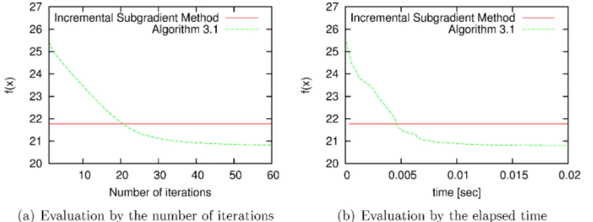
Figure 1 shows the behaviors of$f(x)$ $:= \sum_{i=1}^{N}f_{i}(x)$for the incremental subgradient method

(1.1) and Algorithm 3.1 with a constant step size. The $y$-axis in Figures $1(a)$ and $1(b)$

represent the value of $f(x)$. The $x$-axis in Figure $1(a)$ represents the number of iterations

and the $x$-axis in Figure 1(b) represents the elapsed time. Theresults show that Algorithm

3.1 minimizes the value of $f(x)$ more than the incremental subgradient method _{does (1.1).}

Numberofiterations time$[\sec]$

(a) Evaluation by the number of iterations (b) Evaluation by the elapsed time

FIGURE 1. Behavior of $f(x)$ _for _{the incremental subgradient method and}

Al-gorithm 3.1 with constant step size

Figure 2 shows the behaviors of $f(x)$ for the incremental subgradient method (1.1) and

Algorithm 3.1 withthe diminishing step size. The $y$-axis in Figures 2(a) and 2(b) represent

thevalue of$f(x)$. _The$x$-axisinFigure 2(a) representsthenumber of iterations, and the$x$-axis

in Figure 2(b) represents the elapsed time. The results show that Algorithm 3.1 converges slower than the incrementalsubgradientmethod. However, it shows that Algorithm3.1 with

aconstant stepsize behaves roughly to thesame as the incremental subgradientmethodwith

the diminishing step size. This implies that, if it is diﬃcult to share the diminishing step

size with all users, Algorithm 3.1 can be usedas an eﬀective approximation algorithm of the

incremental subgradient method.

5. CONCLUSION AND FUTURE WORK

This paperdiscussed the problemof minimizingthe sumofnondiﬀerentiable, convex func-tionsover a simple convexclosed constraint set ofareal Hilbert space. It presentedaparallel

(6)

$\hat{arrow\vee X}$

Number ofiterations time$[\sec]$

(a) Evaluation bythenumber ofiterations (b) Evaluation by the elapsed time

FIGURE 2. Behavior of$f(x)$ _with diminishing step size

algorithm for solving theproblem. We studied its convergence properties for aconstant step

size and

a

diminishing step size. We showed that the algorithm with a constant step size approximates a solution to the problem, while the algorithm with

a

diminishing step size weakly converges to a solution to the problem. Finally, we numerically compared the

al-gorithm with the existing algorithm and showed that, when the step size is constant, the

algorithm performs betterthan the existing algorithm.

The numerical comparisons also indicated that, when the step size is diminishing, the

existing algorithmconverges toasolutionfaster thanour algorithm. Therefore, in thefuture,

we should consider developing parallel optimization algorithms which perform better than

the existing algorithm evenwhen the step sizes are diminishing. ACKNOWLEDGMENTS

Theauthors would liketo thank ProfessorWataru Takahashi for givingus achance to

dis-cuss

Problem 2.3in The International Workshop onNonlinear Analysis and ConvexAnalysis held at the Research Institute for Mathematical Sciences, Kyoto University on the 19th of August in 2014.

The authors wouldlike to congratulate Professor Wataru Takahashi on his70th birthday. REFERENCES

[1] Bauschke,H.H.,Borwein, J.M.: On projection algorithms for solvingconvexfeasibility problems. SIAM

Review 38(3), 367-426 (1996)

[2] Bauschke, H.H., Combettes, P.L.: Convex Analysis and Monotone Operator Theory in Hilbert Spaces.

Springer (2011)

[3] Combettes, P.L., Pesquet, J.C.: Proximal splitting methods in signal processing. In: H.H. Bauschke,

R.S. Burachik, P.L. Combettes, V. Elser, D.R. Luke, H. Wolkowicz (eds.) Fixed-Point Algorithms for

(7)

[4] Helou Neto, E.S., De Pierro, A.R.: Incremental subgradients for constrained convex optimization: $A$

unified frameworkandnewmethods. SIAM Journalon optimization 20, 1547-1572 (2009)

[5] _{Hishinuma, K., Iiduka, H.: Parallel subgradient method for nonsmooth} _convex _{optimization with} _a

simple constraint. (submitted)

[6] Iiduka, H.: _{Fixed point optimization algorithms for distributed} _optimization _{in networked systems.} SIAMJournalon optimization 23, 1-26 (2013)

[7] Iiduka,H.,Hishinuma, K.: Acceleration_{method combining broadcast and incremental distributed}

opti-mization algorithms. SIAM Journalon optimization24(4), 1840-1863 (2014)

[8] Message Passing Interface Forum: MPI: A Message-PassingInterface Standard, Version3.0. High

Per-formance Computing Center Stuttgart (2012)

[9] Nedi\v{c}, A., Bertsekas, D.P.: Incremental sugradient methods for nondiﬀerentiable optimization. SIAM

Journalonoptimization 12, 109-138 (2001)

[10] Pesquet, J.C., Pustelnik, N.: Aparallelinertial proximal optimizationmethod. Pacific Journal of Opti-mization8, 273-306 (2012)

[11] Rockafellar, R.T.: Convex Analysis. Princeton University Press (1970)

[12] Solodov, M.V.,Zavriev, S.K.: Error stabilitypropertiesofgeneralizedgradient-type algorithms. Journal of optimization Theory and Applications 98, 663-680 (1998)

[13] Takahashi, W.: Nonlinear Functional Analysis. Yokohama Publishers (2000)

(K.Hishinuma, H.Iiduka)DEPARTMENTOFCOMPUTERSCIENCE, MEIJI UNIVERSITY, 1-1-1 HIGASHIMITA, TAMA-KU, KAWASAK1-SHI, KANAGAWA 214-8571, JAPAN

$E$-mail address, _K. _Hishinuma:

[email protected]$i$.ac.jp