Structure
and stability of
stationary
solutions
to
a
cross-diffusion equation
龍谷大学理工学部 四ツ谷晶二 (Shoji Yotsutani)
Fuculty of Science and Technology,
Ryukoku University
1
Introduction
This is ajoint project withYuan Lou (OhioState University), Wei.-MingNi
(Univer-sity of Minnesota and EastChina NormalUniversity) concerningmathematical analysis,
and Masaharu Nagayama (Hokkaido University), Tatsuki Mori (Ryukoku University)
concerning numerical computation.
In an attempt to model segregation phenomena in population dynamics, Shigesada,
Kawasaki and Teramoto [7] in 1979 incorporated the inter-competition system. In
par-ticular, the following system was proposed
$[Matrix]$
(1.1)where $\Omega$ is a bounded domain $R^{N}(N\geq 1)$ with smooth boundary $\partial\Omega$
.
Here$u$ and $v$
representthe densities of twocompeting species. Theconstants$a_{j},$ $b_{j},$$c_{j}$ and $d_{j}(j=1,2)$
are all positive, where $a_{1},$ $a_{2}$ denote the intrinsic growth rates of these two species,
$b_{1}$ and
$c_{2}$ account for intra-specific competitions while $b_{2},$ $c_{1}$ account for inter-specific
competitions, and$d_{1},$ $d_{2}$ aretheir diffusion rates. Theconstants $\rho_{11},$ $\rho_{22}$ represent
intra-specific population pressures, also known
as
self-diffusion rates, and $\rho_{12},$ $\rho_{21}$ are thecoefficients of inter-specific population pressures, also known
as
cross-diffusion rates.For convenience, we set $A$ $:=a_{1}/a_{2},$ $B$ $:=b_{1}/b_{2},$ $C$ $:=c_{1}/c_{2}$
.
If $B<C$, we call itthe strong competition
case
and $B>C$ the weak competition case.If$\rho_{11}=\rho_{12}=\rho_{21}=\rho_{22}=0$, then (1.1) is the classical Lotka-Volterra competition
diffusion system with Neumann boundary condition
It is well known that in the “weak competition” case, i.e.
$B>A>C,$
the constant steady state $(u_{*}, v_{*})=(ac-acba-b_{2}ab_{1^{C}2}-b_{2}c_{1},b_{1}c_{2}-b_{2}c_{1}$ is globally asymptotically
sta-ble regardless of the diffusion rates $d_{1}$ and $d_{2}$. This implies, in particular, that no
nonconstant steady state can exist for any diffusion rates $d_{1},$ $d_{2}.$
On the other hand, it seems not entirely reasonable to add just diffusions to models
in population dynamics, since individuals do not move around completely randomly. In
particular, while modeling segregation phenomena for two competing species one must
take into account the cross-diffusion pressures
$\{\begin{array}{ll}u_{t}=\Delta[(d_{1}+\rho_{12}v)u]+u(a_{1}-b_{1}u-c_{1}v) , in \Omega\cross(O, \infty) ,v_{t}=\Delta[(d_{2}+\rho_{21}u)v]+v(a_{2}-b_{2}u-c_{2}v) , in \Omega\cross(O, \infty) ,\underline{\partial u}=\underline{\partial v}=0, on\partial\Omega\cross(0, \infty) ,\partial n \partial n u(x, O)=u_{0}(x), v(x, 0)=v_{0}(x) , in \Omega.\end{array}$ (1.3)
Mimura and his collaborators started mathematical analysis around 1980 (see, e.g.
Mimura [4]$)$. Considerable work has been doneconcerning the global existence of
solu-tions to systems (1.3) under various hypotheses. $A$ priori estimates are crucial to obtain
the global existence. As for recent progress including stationary problems,
see
Ni [5], Ni[6], Yagi[9] and Yamada [10].
2
Limiting equation
We first focus on the effect of cross-diffusion on steady states. To illustrate the
significanceof cross-diffusions, we again go to the weak competition case (i.e. $B>A>$
$C)$ since in this
case
(1.3) has no nonconstant steady states if both $\rho_{12}=\rho_{21}=0$.
Lou-Ni [1],[2] show that, indeed, if one ofthe twocross-diffusion rates, say$\rho_{12}$, is large, then
(1.3) will have nonconstant steady states provided that $d_{2}$ belongs to a proper range.
On the other hand, if both $\rho_{12}$ and $\rho_{21}$ are small, then (1.3) will have no nonconstant
steadystates under the condition
$B>A>C$
.
This shows the cross-diffusiondoes seemto help create patterns.
In the strong competition case, i.e.
$B<A<C$
, even the situation of steady statessolutions of (1.2) becomes more interesting. Cross-diffusion still have similar effects in
The following two theorem are due to Lou-Ni [1], [2].
Theorem 2.1 $([2J)$ Suppose
for
simplicity that$\rho_{21}=0$. Supposefurther
that$B\neq A\neq$$C,$ $n\leq 3$ and $\frac{a_{2}}{d_{2}}\neq\lambda_{k}$
for
any $k\geq 1$, where $\lambda_{k}$ is the $kth$ eigenvalueof
$-\triangle$ on $\Omega$with
zero
Neumann boundary data. Let $(u_{j}, v_{j})$ be a nonconstant steady state solutionof
(1.3) with $\rho_{12}=\rho_{12,j}$. Then by passing to a subsequenceif
necessary, either (i)of
(ii) holds as $\rho_{12,j}arrow\infty$:
(i) $(u_{j}, \frac{\rho_{12,j}}{d_{1}}v_{j})arrow(u, v)$ uniformly, $u>0,$ $v>0$, and
$\{\begin{array}{ll}d_{1}\Delta[(1+v)u]+u(a_{1}-b_{1}u)=0 in \Omega,d_{2}\triangle v+v(a_{2}-b_{2}u)=0 in \Omega,\frac{\partial u}{\partial n}=\frac{\partial v}{\partial n}=0 on\partial\Omega.\end{array}$
(ii) $(u_{j}, v_{j}) arrow(\frac{\tau}{v}, v)$ uniformly, $\tau$ is
a
positive constant, $v>0$, and$\{\begin{array}{l}\int_{\Omega}\frac{\tau}{v}(a_{1}-b_{1}\frac{\tau}{v}-c_{1}v)dx=0,d_{2}\triangle v+v(a_{2}-c_{2}v)-b_{2}\tau=0 in \Omega,\frac{\partial v}{\partial n}=0, on\partial\Omega.\end{array}$ (2.1)
Their proofs of obtaining the above limiting equations are quite hard and lengthy.
The most important step in the proof is to obtain a priori bounds on steady states of
(1.3) that
are
independent of $\rho_{12}.$It seems from numerical computations that solutions of the case (i) is not directly
related withstable solutions of the original equation withsufficientlylarge$\rho_{12}$
.
However,we observenumerically that solutionsof the case (ii) is closely related with the original
equationwith sufficiently large $\rho_{12}.$
Thus, wewill concentrate on the case (ii). Now, we consider the 1-dimensional case
with $\Omega=(0,1)$. The limiting equation becomes
as
follows:3
Structure
and
stability
in
1-dimensional
case
Due to the scaling and reflection properties of solutions to autonomous ordinary
differential equations, all solutions to the (2.2) are obtained by several reflections and a
suitable re-scaling from solutions of the following system:
$\{\begin{array}{l}\int_{0}^{1}\frac{1}{v}(a_{1}-b_{1^{\frac{\tau}{v}}})dx-c_{1}=0,d_{2}v_{xx}+v(a_{2}-b_{2}\frac{\tau}{v}-c_{2}v)=0 in (0,1) ,v_{x}(0)=v_{x}(1)=0,v>0, and v_{x}>0, in(O, l).\end{array}$ (3.1)
Now, we will discuss about the structure ofstationary solutions and their stability.
This system (3.1) consists ofa nonlinearelliptic equation and an integral constraint.
As far
as
existence and non-existence in one dimensional domainare
concemed,Lou-Ni-Yotsutani [3] obtained nearly complete knowledge. They also obtained the precise
qualitative behavior of solutions to this limiting system
as
the diffusion rate varies.Their basic approach is to convert the problem of solving the system to a problem
of solving its “representation” in a different parameter space. This is first done without
the integral constraint, and then they use the integral constraint to find the “solution
curve” in the new parameter space. This tums out to be a powerful method
as
it givesfairly precise information about the solutions.
We have recently made clear the remained delicate parts due to the exphcit
repre-sentation by elliptic functions.
We summarized the structure of solutions of (3.1). We concentrate on the
case
$B<C$ (strong competition case).
The following two theorem are due to [3].
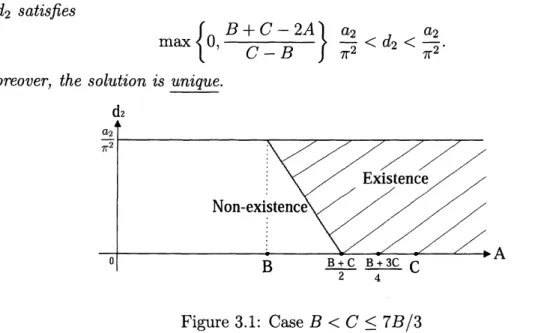
Theorem 3.1 (Existence) Suppose that $B<C$.
If
$\max\{0, \frac{B+C-2A}{C-B}\}\frac{a_{2}}{\pi^{2}}<d_{2}<\frac{a_{2}}{\pi^{2}},$
then there exists a solution $(v(x), \tau)$
of
(3.1).Theorem 3.2 (Nonexistence) Suppose that $B<C.$
(i)
If
$d_{2} \geq\frac{a_{2}}{\pi^{2}}$, then there exists no solutionof
(3.1).(iii)
If
$A<B$, there exists no solutionof
(3.1).(iii)
If
$B \leq A<\frac{B+C}{2}$, then there exists a $d_{2}^{*}=d_{2}^{*}(A, B, C, a_{2})>0$ such thatWe see that the above theorem is sharp by the following theorems. The existence
regiondependingonthethe ratio$C/B$
.
Thesituation drastically changes at $C/B=7/3.$Theorem 3.3 Suppose that $B<C\leq 7B/3$. (3.1) has a solution $(v(x), \tau)$
if
and onlyif
$d_{2}$satisfies
$\max\{0, \frac{B+C-2A}{C-B}\}\frac{a_{2}}{\pi^{2}}<d_{2}<\frac{a_{2}}{\pi^{2}}.$
Moreover, the solution is unique.
Figure 3.1: Case $B<C\leq 7B/3$
Theorem 3.4 Suppose that $7B/3<C.$ $(3.1)$ has the unique solution $(v(x), \tau)$
if
$\max\{0, \frac{B+C-2A}{C-B}\}\frac{a_{2}}{\pi^{2}}<d_{2}<\frac{a_{2}}{\pi^{2}}.$
Moreover, there exists the only one connected non-empty open set $D$ with
$D\subset\{(A, d_{2})$ : $B<A< \frac{B+C}{2},$ $0<d_{2}< \{\frac{B+C-2A}{C-B}\}\frac{a_{2}}{\pi^{2}}\}$
such that (3.1) has exactly two solutions $(v(x), \tau)$
if
and onlyif
$d_{2}\in D.$The following theorems in [3] give the shape of solutions to (3.1)
as
$d_{2}\uparrow a_{2}/\pi^{2}.$Theorem 3.5 (Shape of solutions
as
$d_{2}\uparrow a_{2}/\pi^{2}$ ) Suppose that $B<C.$Let $(v(x, d_{2}), \mathcal{T}(d_{2}))$ be solutions
of
(3.1).If
$A\geq B$, then $v(x;d_{2})arrow 0,$ $\frac{v(x;d_{2})-v(0;d_{2})}{v(1;d_{2})-v(0;d_{2})}arrow\frac{1-\cos(\pi x)}{2},$$\frac{\tau(d_{2})}{v(x;d_{2})}arrow\frac{a_{2}}{b_{2}}\cdot\frac{1}{1-\sqrt{1-\frac{B}{A}}\cos(\pi x)}$
uniformly on $[0,1]$ as $d_{2}\uparrow a_{2}/\pi^{2}.$
Figure 3.3: $u$
as
$d_{2}\uparrow a_{2}/\pi^{2}$ Figure 3.4: $v$ as $d_{2}\uparrow a_{2}/\pi^{2}$The following theorems in [3] give the shape of solutions to (3.1) as $d_{2}\downarrow 0.$ $A$ new
number $(B+3C)/4$ appears. The shape is drastically change at $A=(B+3C)/4$
Theorem 3.6 (Shape ofsolutions
as
$d_{2}arrow 0$ for $A< \frac{B+3C}{4}$ ) Suppose that $B\neq C$. Let$(v(x, d_{2}), \tau(d_{2}))$ be solutions
of
(3.1).If
$A< \frac{B+3C}{4}$ and $B<C$, then$v( O;d_{2})arrow 2\cdot\frac{a_{2}}{c_{2}}\cdot\frac{\frac{B+3C}{4}-A}{C-B},$ $v(x;d_{2}) arrow\frac{a_{2}}{c_{2}}\cdot\frac{A-B}{C-B}$ for $x>0,$
$\frac{\tau(d_{2})}{v(0;d_{2})}arrow\frac{a_{2}}{2c_{2}}\cdot\frac{C-A}{C-B}\cdot\frac{A-B}{\frac{B+3C}{4}-A},$ $\frac{\tau(d_{2})}{v(x;d_{2})}arrow\frac{a_{2}}{b_{2}}\cdot\frac{C-A}{C-B}$ for $x>0,$
as
$d_{2}\downarrow 0.$Theorem 3.7 (Shape ofsolutions as $d_{2}arrow 0$ for $A \geq\frac{B+3C}{4}$ ) Suppose that $B\neq C$. Let $(v(x, d_{2}), \tau(d_{2}))$ be solutions
of
(3.1).If
$B<C$ and$A \geq\frac{B+3C}{4}$, then$v(0;d_{2})arrow 0,$ $v(x;d_{2}) arrow\frac{3a_{2}}{4c_{2}}$ for $x>0,$
$\frac{\tau(d_{2})}{v(0;d_{2})}arrow\infty,$ $\frac{\tau(d_{2})}{v(x;d_{2})}arrow\frac{a_{2}}{4c_{2}}$ for $x>0$, as $d_{2}arrow 0.$
Figure 3.7: $u$ for $(B+3C)/4<A$ Figure 3.8: $v$ for $(B+3C)/4<A$
4
Stability
in one-dimensional
problem
Let us consider the stability of stationary solutions, and multi-dimensional solutions
withtheir stability.
Time dependent limiting equation is as follow. Unknown functions are $\tau(t),$ $v(x, t)$,
and
$\{\begin{array}{l}\frac{d}{dt}(\int_{\Omega}\frac{\tau}{v}dx)=\int_{\Omega}\frac{\tau}{v}(a_{1}-b_{1}\frac{\tau}{v}-c_{1}v)dx,\frac{\partial v}{\partial t}=d_{2}\triangle v+v(a_{2}-c_{2}v)-b_{2}\tau in \Omega,\frac{\partial v}{\partial n}=0 on\partial\Omega.\end{array}$
We suspect from a lot of numerical computation that the equation is a nice
approxi-mation of the original time dependent problem with sufficiently large $r$ $:=\rho_{12}/d_{1}$
.
Forinstance, for $r=700,000$, it is not easy to distinguish each other.
The following Figure 4.1 shows numerical results for
$d_{1}=1, d_{2}=*, r=700,000$
$a_{2}=*, b2=1, c2=2.$ $a_{2}=1, b2=1, c2=1.$
We note that $C<7B/3,$ $(B+C)/2=1.5$ and $(B+3C)/4=1.75$ , since $B=1$ and
Figure 4.1: Stability and instability
Wu[8] gavea proof ofinstability for
$d_{2}$ sufficiently small with
$(B+C)/2<A<(B+4C)/4$
in one-dimensional
case.
Recently, she have also given a proofof stability for$d_{2}(<a_{2}/\pi^{2})$ sufficiently close to $a_{2}/\pi^{2}$ with
$(B+C)/2<A<(B+4C)/4$
in one-dimensional case.
5
Multi-dimensional
problem
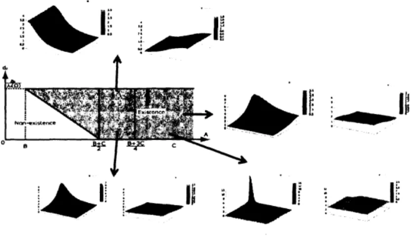
We have done various numerical computations for the
case
$\Omega$ is rectangles in2-dimensional space. It
seems
that thestructure of stable stationary solutions is essentiallyvery similar to 1-dimensional case, though there are muchvarietiesof shape of solutions
in 2-dimensional case than in one-dimensional case.
Now, we will state some mathematical results. We prepare notations. Let
$\lambda_{0}=0<\lambda_{1}\leq\lambda_{2}\leq\cdots$
$\varphi_{0}=$ const.
$,$ $\varphi_{1},$ $\varphi_{2},$
$\cdots$
be eigen values and corresponding eigen functions $of-\triangle$ in $\Omega\subset R^{N}$ with Neumann
boundary.
Theorem 5.1 Suppose that $N\leq 3$ and $\lambda_{1}$ be a simple eigen values with an eigen
function
$\varphi_{1}$.
Then, there exists exactly two positive non-constant solutions $(v_{-}, \tau_{-})$ and$(v_{+}, \tau_{+})$
of
(2.1)for
$d_{2}$ sufficiently close to $a_{2}/\lambda_{1}$ with $d_{2}<a_{2}/\lambda_{1}$Moreover,
$\tauarrow 0,$
$\frac{\tau_{\pm}(d_{2})}{v_{\pm}(x;d_{2})}arrow\frac{a_{2}}{b_{2}}\cdot\frac{1}{1+\mu\pm\varphi_{1}(x)}$
as $d_{2}\uparrow a_{2}/\lambda_{1}$, where
$\mu_{-},$$\mu+(\mu_{-}<0<\mu_{+})$ are solutions
of
$\frac{\int_{\Omega}(1+\mu\varphi_{1}(x))^{-2}dx}{\int_{\Omega}(1+\mu\varphi_{1}(x))^{-1}dx}=\frac{A}{B}.$
Remark. The set $\{(v_{-}, \tau_{-}), (v_{+}, \tau_{+})\}$ is uniquely determined though there is a
freedom
to pick up $\varphi_{1}$
.
The condition $N\leq 3$ comes from Harnack’s inequality in our proof.Remark. For$N=1,$ $\Omega=(0,1)$, it is easy to see that
$\lambda_{1}=\pi^{2}, \varphi_{1}(x)=\cos\pi x, \frac{1}{1-\mu^{2}}=\frac{A}{B}, \mu\pm=\pm\sqrt{1-\frac{B}{A}}.$
Remark. For$N=2,$ $\Omega=(0,1)\cross(0, \ell)$ with $0<\ell<1$, it is easy to see that
$\lambda_{1}=\pi^{2}, \varphi_{1}(x, y)=\cos\pi x, \frac{1}{1-\mu^{2}}=\frac{A}{B}, \mu\pm=\pm\sqrt{1-\frac{B}{A}}.$
Theorem 5.2 Suppose that $N\leq 3$ and $\lambda_{1}$ be a simple eigen values. Then, $(v_{-}, \tau_{-})$
and $(v_{+}, \tau_{+})$
defined
by Theorem 5.1 are asymptotically stablefor
$d_{2}$ sufficiently close to$a_{2}/\lambda_{1}$ with $d_{2}<a_{2}/\lambda_{1}.$
The following general lemmaplays crucial role to prove Theorems 5.1 and 5.2.
Lemma 5.3 Suppose that$N\geq 1$ and $\varphi_{1}$ be eigen values corresponding to $\lambda_{1}$
.
Let $g(\mu)$$g( \mu);=\frac{\int_{\Omega}(1+\mu\varphi_{1}(x))^{-2}dx}{\int_{\Omega}(1+\mu\varphi_{1}(x))^{-1}dx}$
$for \mu\in(-1/\max_{\overline{\Omega}}\varphi_{1}, -1/\min_{\overline{\Omega}}\varphi_{1})$
.
Then$\frac{dg(\mu)}{d\mu}=\{\begin{array}{ll}+ for \mu>0,0 for\mu=0,- for \mu<0.\end{array}$
Moreover,
for
$N\leq 4,$$\{\begin{array}{l}g(\mu)arrow\infty as \mu\uparrow\mu_{+},g(\mu)arrow\infty as \mu\downarrow\mu_{-}.\end{array}$
References
[1] Y. Lou andW. M. Ni, Diffusion,
self-diffusion
and cross-diffusion, J. DifferentialEquations, 131 (1996), 79-131.
[2] Y. Lou and W. M. Ni,
Diffusion
vscross-diffusion:
An elliptic approach, J.Differential Equations, 154 (1999), 157-190.
[3] Y. Lou, W. M. Ni and S. Yotsutani, On a limiting system in the Lotka-Volterra
competitionwith cross-diffusion, Discrete Contin. Dyn. Syst, 10 (2004), 435-458.
[4] M.Mimura Stationarypattem
of
some density-dependentsystemwith competitivedynamics, Hiroshima Math. J. 8 (1981), 621-635.
[5] W. M. Ni, Diffusion, cross-diffusion, and theirspike-layersteady states, Notices
Amer. Math. Soc., 45 (1998), 9-18.
[6] W. M. Ni, The Mathematics
of
Diffusion, CBMS-NSF Regional ConferenceSeries in Applied Mathematics, 82 (2011), SIAM.
[7] N. Shigesada, K. Kawasaki and E. Teramoto, Spatial $\mathcal{S}$egregation
of
intemctingspecies, J. Theor. Biol., 79 (1979), 83-99.
[8] Y. Wu, The instability
of
spiky steady statesfor
a competing species model withcross
diffusion, J. Differential Equations, 213 (2005), 289-340.[9] A. Yagi, Abstmct Pambolic Evolution Equations and their Applications, 2009,
Springer.
[10] Y. Yamada, Nonlinear