HIGHER-ORDER ALEXANDER INVARIANTS FOR HOMOLOGICALLY FIBERED KNOTS (Intelligence of Low-dimensional Topology)

(1)

HIGHER-ORDER ALEXANDER INVARIANTS FOR HOMOLOGICALLY FIBERED KNOTS

HIROSHI GODA AND TAKUYA SAKASAI

1. INTRODUCTION

Thisnoteisadaptedfrom the talk atthe 2010Intelligenceof Low-dimensional Topology

at Research Institutefor Mathematical Sciences, Kyoto University. For the detail,

see

the

original papers [12], [13].

Let $\Sigma_{g,n}$ be a compact oriented surface of genus $g$ with $n\geq 1$ boundary components,

and the triple $(M, i_{+}, i_{-})$ be an oriented homology cobordism between $\Sigma_{g,n}$ and $\Sigma_{g,n}$ with

two markings of$\partial M$ : $i_{+},$$i_{-}:\Sigma_{g,1}\mapsto\partial M$

.

We call $(M, i_{+}, i_{-})$

a

homology cylinder

over

$\Sigma_{g,n}$

.

This object

was

introduced by Goussarov [14] and Habiro [16] since it is suitable

for applying the theory of clovers and claspers, and then has been studied together with finite type invariants of 3-manifolds. The following have been known

as

methods for constructing homology cylinders:

$\bullet$ connected

sums

of the trivial cobordism with homology 3-spheres; $\bullet$ Levine’s method [19] using string links in the 3-ball;

$\bullet$ Habegger $s$ method [15] giving homology cylinders

as

results of surgeries along

string links in homology 3-balls; and

$\bullet$ clasper surgeries (see [14] and [16]).

In [12], the authors gave anexplicit construction of homology cylinders, i.e.

we

introduced

a

notion of

a

homologically

_fibered

knot and construct

a

homology cylinder using it. The family of the homologically fibered knots include that of the fibered knots. So, roughly speaking, the following relationships exist:

Pure_{$\cap Braid$} $rightarrow$

$Mapping\cap$cylinder $Fibered\cap$ knot

Pure String link $\underline{Levin}e$

Homology cylinder Homologically fibered knot

(Habegger-Lin) (Goussarov, Habiro)

In [18], Kirk-Livingston-Wang introduced a Reidemeister torsion for string links, then

the second author studied the corresponding Reidemeister torsion for homologycylinders

in [23]. Note that this torsion may be regarded

as

aspecial

case

of

a

decatogorification of sutured Floer homology [8]. In thisnote, we study the Reidemeistertorsion for

homologi-callyfibered knots and show afactorization formula. Further, wegive a MATHEMATICA

program for explicit calculations of the invariants for homologically fibered knots.

2000 Mathematics Subject _{Classification.} Primary$57M27$_{, Secondary}$57M25$.

The authors are partially supported by Grant-in-Aid for Scientific Research, (No. 21540071 and No. 21740044), MinistryofEducation, Science, Sports and Technology, Japan.

(2)

2. HOMOLOGICALLY FIBERED KNOTS

In this section,

we

introduce two main objects in this note: homology cylinders and sutured manifolds. First, we define homology cylinders

over

surfaces, which have their originin Goussarov [14], Habiro [16], Garoufalidis-Levine [11] and Levine [19]. Let $\Sigma_{g,n}$ be

a

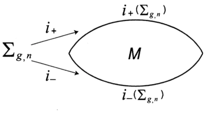
compact connected oriented surface ofgenus $g\geq 0$ with $n\geq 1$ boundary components.

Definition 2.1. A homology cylinder $(M, i_{+}, i_{-})$

over

$\Sigma_{g,n}$ consists of

a

compactoriented

3-manifold $M$ with two embeddings $i_{+},$$i_{-}:\Sigma_{g,n}\mapsto\partial M$ such that:

(i) $i_{+}$ is orientation-preserving and $i_{-}$ is orientation-reversing;

(ii) $\partial M=i_{+}(\Sigma_{g,n})\cup i_{-}(\Sigma_{g,n})$ and $i_{+}(\Sigma_{g,n})\cap i_{-}(\Sigma_{g,n})=i_{\dagger}(\partial\Sigma_{g,n})=i_{-}(\partial\Sigma_{g,n})$;

(iii) $i_{+}|_{\partial\Sigma_{g,n}}=i_{-}|_{\partial\Sigma_{g,n}}$; and

(iv) $i_{+},$$i_{-}:H_{*}(\Sigma_{g,n};\mathbb{Z})arrow H_{*}(M;\mathbb{Z})$

are

isomorphisms.

If

we

replace (iv) with the condition that $i_{+},$$i_{-}:H_{*}(\Sigma_{g,n};\mathbb{Q})arrow H_{*}(M;\mathbb{Q})$

are

isomor-phisms, then $(M, i_{+}, i_{-})$ is called a rational homology cylinder.

$i_{+}( \sum_{g,n})$

$i_{-}( \sum_{g,n})$

FIGURE 1. Homology cylinder

We often write

a

(rational) homology cylinder $(M, i_{+}, i_{-})$ briefly by $M$

.

Note that

our

definition is the

same

as that in [11] and [19] except that we may consider homology cylinders

over

surfaces with multiple boundaries.

Two (rational) homology cylinders $(M, i_{+}, i_{-})$ and $(N, j+, j_{-})$ over $\Sigma_{g,n}$ are said to be

isomorphicif there exists

an

orientation-preserving diffeomorphism $f$ : $Marrow N\underline{\simeq}$satisfying

$j+=foi_{+}$ and$j_{-}=foi_{-}$. Wedenote the set of isomorphism classesofhomology cylinders

(resp. rational homology cylinders) over $\Sigma_{g,n}$ by $C_{g,n}$ (resp. $C_{g,n}^{\mathbb{Q}}$).

Example 2.2 (Mapping cylinder). For each diffeomorphism $\varphi$ of $\Sigma_{g,n}$ which fixes $\partial\Sigma_{g,n}$

pointwise (hence, $\varphi$ preserves the orientation of$\Sigma_{g,n}$), we can construct ahomology

cylin-der by setting

$(\Sigma_{g,n}\cross[0,1], id\cross 1, \varphi\cross 0)$,

where collars of $i_{+}(\Sigma_{g,n})$ and $i_{-}(\Sigma_{g,n})$

are

stretched half-way along $(\partial\Sigma_{g,n})\cross[0,1]$. It is easily checked that the isomorphism class of $(\Sigma_{g,n}\cross[0,1], id\cross 1, \varphi\cross 0)$ depends only

on

the (boundary fixing) isotopy class of $\varphi$. Therefore, this construction gives a map from

(3)

Next, we recall the definition of sutured manifolds given by Gabai [10]. We here

use a

special

case

of them.

A sutured

_manifold

$(M, \gamma)$ is

a

compact oriented 3-manifold $M$ together with

a

subset

$\gamma\subset\partial M$ which is

a

union offinitely many mutually disjoint annuli. For each component

of$\gamma$,

an

oriented

core

circle called

a

suture is fixed, and

we

denote the set of sutures by

$s(\gamma)$. Every component of$R(\gamma)=\partial M$-Int$\gamma$ is oriented

so

that the orientations

on

$R(\gamma)$

are

coherent with respect to $s(\gamma)$, that is, the orientation of each component of $\partial R(\gamma)$

induced from that of $R(\gamma)$ is parallel to the orientation of the corresponding component

of$s(\gamma)$. We denote by $R_{+}(\gamma)$ (resp. $R_{-}(\gamma)$) the union of those components of$R(\gamma)$ whose normal vectors point out of (resp. into) $M$.

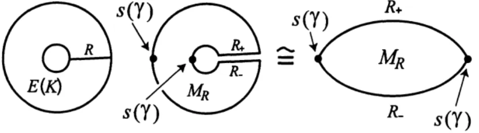
Example 2.3. For

a

knot $K$ in $S^{3}$ and

a

Seifert surface $\overline{R}$ of_$K$,

we

set _{$R:=\overline{R}\cap E(K)$},

called also

a

Seifert surface, where $E(K)=\overline{S^{3}-N(K)}$ is the complement of a regular

neighborhood $N(K)$ of$K$. Then $(M_{R}, \gamma)$ $:=(\overline{E(K)-N(R)}, \overline{\partial E(K)-N(\partial R)})$ defines

a

sutured manifold. We call it the complementary sutured

_manifold

for $R$

.

In this paper,

we simply call it the sutured manifold for $R$

.

FIGURE 2. Complementary sutured manifold

Let $L$ be an oriented link in the 3-sphere $S^{3}$, and $\triangle_{L}(t)$ the normalized (one variable)

Alexander polynomial of$L$, i.e. the lowest degree of$\Delta_{L}(t)$ is $0$

.

Definition 2.4. An n-component link $L$ in $S^{3}$ is said to be homologically

fibered

if $L$

satisfies the following two conditions:

(i) The degree of $\Delta_{L}(t)$ is $2g+n-1$, where $g$ is the genus of

a

connected Seifert

surface of$L$; and

(ii) $\Delta_{L}(0)=\pm 1$

.

If

an

n-component link$L$ satisfies (i), then $L$ is said to be rationally homologically

fibered.

The Alexander polynomial that satisfies the condition (ii) is said to be monic in this paper.

Remark 2.5. In general, if $L$ bounds a connected Seifert surface ofgenus $g$, then

$2g+n-1\geq$ (the degree of$\triangle_{L}(t)$).

It is known ([5], [21]) that if $L$ has

an

alternating diagram that gives, by the Seifert

algorithm, a connected Seifert surface ofgenus $g$, then the degree of $\Delta_{L}(t)$ is equal to $2g+n-1$

.

(4)

Remark 2.6. Suppose $L$ is an alternating link. Then, $L$ isfibered if and only if$\triangle_{L}(t)$ is

monic, by Murasugi [22] (see also 13.26 (c) in [1]). Therefore, if a homologically fibered

link $L$ is not fibered, then $L$ is non-alternating.

Let $L$ be

an

n-component link and $\Sigma_{g,n}$ the compact oriented surface that is

diffeo-morphic to

a

Seifert surface $R$ of $L$

.

We fix

a

diffeomorphism $\theta$ : $\Sigma_{g,n}arrow\underline{\simeq}R$ and denote

by $(M_{R}, \gamma)$ the complementary sutured manifold for $R$. Then we may see that there

are an orientation-preserving embedding $i+:\Sigma_{g,n}arrow M_{R}$ and an orientation-reversing

embedding $i_{-}:\Sigma_{g,n}arrow M_{R}$ with $i_{+}(\Sigma_{g,n})=R_{+}(\gamma)$ and $i_{-}(\Sigma_{g,n})=R_{-}(\gamma)$, where two

embeddings $i\pm$

are

the composite mappings of$\theta$ and embeddings _{$\iota\pm:R\mapsto M_{R}$} such that

$i_{\pm}=\iota_{\pm}0\theta:\Sigma_{g,n}arrow R_{\pm}(\gamma)\subset M_{R}$:

$\Sigma_{g,n}arrow^{\theta}R$

$\backslash _{i\pm}\downarrow\iota\pm$

$M_{R}$

If$i_{+},$ $i_{-}:H_{1}(\Sigma_{g,n})arrow H_{1}(M_{R})$

are

isomorphisms,

we

mayregard $(M_{R}, \gamma)$

as a

homology cylinder. The next proposition was essentially mentioned in [6]. A proof is given in [12]. Proposition 2.7. Let $R$ be a

Seifert

surface of

a link L.

If

the complementary sutured

manifold for

$R$ is a homology cylinder, then $L$ is homologically

fibered.

Conversely,

if

$L$

is homologically fibered, then the complementary sutured

_{manifold for}

each minimalgenus

Seifert surface of

$L$ is a homology cylinder.

It is known that all homologicallyfibered knots are fibered among prime knots with at

most 11 crossings. On the other hand, Friedl-Kim [9] (see also [2]) showed that there are

13 non-fibered homologically fibered knots with 12-crossings. See Figure 7.

3. FACTORIZATION FORMULAS OF ALEXANDER lNVARlANTS

Let $R$be aminimalgenus Seifert surfaceofarationally homologically fibered knot $K$ in

$S^{3}$, and _{$M_{R}$}be the sutured manifold for_{$R\cong\Sigma_{g,1}$}. We fixabasis of$H_{1}(R;\mathbb{Q})$, which yields

anisomorphism$H_{1}(R;\mathbb{Q})\cong \mathbb{Q}^{2g}$. Thenwe canrewrite the definition $\triangle_{K}(t)=\det(S-tS^{T})$

of the Alexander polynomial of$K$ by using theinvertibility (over $\mathbb{Q}$) ofthe Seifert matrix

$S$, and obtain a factorization

(3.1) $\triangle_{K}(t)=\det(S)\det(I_{2g}-t\sigma(M_{R}))$

of$\triangle_{K}(t)$

.

Note that $\sigma(M_{R})$ $:=S^{-1}S^{T}$ represents the composite ofisomorphisms

$\mathbb{Q}^{2g}\cong H_{1}(R;\mathbb{Q})arrow H_{1}(M_{R};\mathbb{Q})i-\underline{\simeq}\vec{i_{+}^{-1}}\underline{\simeq}H_{1}(R;\mathbb{Q})\cong \mathbb{Q}^{2g}$

.

The matrix $\sigma(M_{R})$ can be interpreted as a monodromy of $M_{R}$ from a view point of the

rational homology. Regarding the formula (3.1)

as a

basic case,

we

constructed in [12] its generalization under the framework of higher-order Alexander invariantsdue to Cochran

[3], Harvey [17] and Friedl [7]. In this procedure, the Seifert matrix $S$, the monodromy

(5)

matrix $r_{\rho}(M_{R})$ and

some

higher-order (non-commutative) Reidemeister torsion $\tau_{\rho}(E(K))$

associated with

a

representation $\rho$ of the fundamental group of$M_{R}$

.

Here, we review higher-order Alexander invariants quickly. Fora matrix $A$ with entries

in a group ring $\mathbb{Z}G$ (or its quotient field) for a group $G$, we denote by $\overline{A}$ the matrix

obtained from $A$ by applying the involution induced from $(x\mapsto x^{-1}, x\in G)$ to each

entry. For

a

module $M$,

we

write $M^{n}$ for the module of column vectors with _$n$ entries.

For

a

finite cell complex $X$,

we

denote by $\tilde{X}$

its universal covering. We take

a

base point

$p$ of $X$ and a lift $\tilde{p}$ of

$p$

as a

base point of

$\tilde{X}$

.

$\pi$ $:=\pi_{1}(X,p)$ acts

on

$\tilde{X}$

from the right through its deck transformation group,

so

that the lift of

a

loop $l\in\pi$ starting from $\tilde{p}$

reaches $\tilde{p}l^{-1}$. Then the cellular chain complex $C_{*}(\tilde{X})$ of$\tilde{X}$ becomes

a

right $\mathbb{Z}\pi$-module.

For each left $\mathbb{Z}\pi$-algebra $\mathcal{R}$, the twisted chain complex _{$C_{*}(X;\mathcal{R})$} is given by the tensor

product ofthe right $\mathbb{Z}\pi$-module

C.

$(\tilde{X})$ and the left $\mathbb{Z}\pi$-module $\mathcal{R}$,

so

that _{$C_{*}(X;\mathcal{R})$} and

$H.(X;\mathcal{R})$ are right $\mathcal{R}$-modules.

In the definition of higher-order Alexander invariants, PTFA groups play important

roles, where

a

group $\Gamma$ is said to be poly-torsion-free abelian (PTFA) if it has a sequence

$\Gamma=\Gamma_{0}\triangleright\Gamma_{1}\triangleright\cdots\triangleright\Gamma_{n}=\{1\}$

whose successive quotients $\Gamma_{i}/\Gamma_{i+1}(i\geq 0)$ are all torsion-free abelian. An advantage of

usingPTFA groups is that the group ring $\mathbb{Z}\Gamma$ $($or $\mathbb{Q}\Gamma)$ of$\Gamma$ is known to be an Ore domain

so that it can be embed into the field (skew field in general)

$\mathcal{K}_{\Gamma}:=\mathbb{Z}\Gamma(\mathbb{Z}\Gamma-\{0\})^{-1}=\mathbb{Q}\Gamma(\mathbb{Q}\Gamma-\{0\})^{-1}$

called the right

_field

_{of fractions.}

A typical example ofPTFA groups is $\mathbb{Z}^{n}$, where $\mathcal{K}_{\mathbb{Z}^{n}}$ is

isomorphic to the field ofrational functions with $n$ variables.

For a rationally homologically fibered knot $K$, we take a homomorphism $\rho$ : $G(K)$ $:=$

$\pi_{1}(E(K))arrow\Gamma$ whose target $\Gamma$ is PTFA. We suppose that

$\rho$ is non-trivial. We regard $\mathcal{K}_{\Gamma}$

as a

local coefficient system

on

$E(K)$ through $\rho$.

Lemma3.1 (Cochran [3,Lemma 3.9]). For any non-trivial homomorphism$\rho:G(K)arrow\Gamma$

to a PTFA group $\Gamma$,

we

have _{$H_{*}(E(K);\mathcal{K}_{\Gamma})=0$}

.

By this lemma, we can define the Reidemeister torsion

$\tau_{\rho}(E(K))$ $:=\tau(C_{*}(E(K);\mathcal{K}_{\Gamma}))\in K_{1}(\mathcal{K}_{\Gamma})/\pm\rho(G(K))$

for the acyclic complex$C_{*}(E(K);\mathcal{K}_{\Gamma})$. We refer to Milnor [20] for generalities oftorsions.

By higher-order Alexander invariants for $K$, we here mean this torsion $\tau_{\rho}(E(K))$.

We now describe afactorization of$\tau_{\rho}(E(K))$ generalizing (3.1). Let $(M_{R}, i_{+}, i_{-})\in C_{g,1}^{\mathbb{Q}}$

be the rational homology cylinder obtained as the sutured manifold for a minimal genus

Seifert surface $R$ of$K$

.

We

use

the

same

notation $\rho$ : $\pi_{1}(M_{R})arrow\Gamma$ for the composition

$\pi_{1}(M_{R})arrow G(K)arrow^{\rho}\Gamma$

.

Applying Cochran-Orr-Teichner [4, Proposition 2.10], we have

the following:

Lemma 3.2. $i_{+},$$i_{-}:H_{*}(\Sigma_{g,1},p;i_{\pm}^{*}\mathcal{K}_{\Gamma})arrow H_{*}(M_{R},p;\mathcal{K}_{\Gamma})$ are isomorphisms as right $\mathcal{K}_{\Gamma^{-}}$

(6)

This lemma provides the followingtwo kinds of invariants for $M_{R}$.

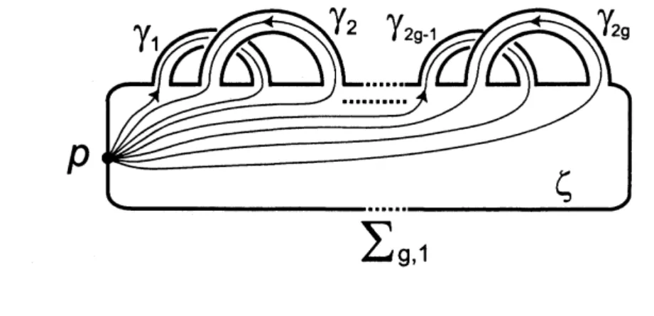
The Magnus matrix Let $X\subset\Sigma_{g,1}$ be the bouquet of$2g$circles $\gamma_{1},$

$\ldots,$$\gamma_{2g}$ tied at$p$ (see

Figure 3). $X$ is

a

deformation retract of $\Sigma_{g,1}$ relative to_$p$

.

Therefore, for $\pm\in\{+, -\}$,

we

have

$H_{1}(\Sigma_{g,1},p;i_{\pm}^{*}\mathcal{K}_{\Gamma})\cong H_{1}(X,p;i_{\pm}^{*}\mathcal{K}_{\Gamma})=C_{1}(\tilde{X})\otimes_{\pi 1(\Sigma_{g,1})}i_{\pm}^{*}\mathcal{K}_{\Gamma}\cong \mathcal{K}_{\Gamma}^{2g}$

with a basis

$\{\tilde{\gamma}_{1}\otimes 1, \ldots, \tilde{\gamma}_{2g}\otimes 1\}\subset C_{1}(\tilde{X})\otimes_{\pi_{1(\Sigma_{g,1})}}i_{\pm}^{*}\mathcal{K}_{\Gamma}$

as a right $\mathcal{K}_{\Gamma}$-vector space. Here we fix a lift $\tilde{p}$of

$p$ as a base point of

$\tilde{X}$, and

denote by

$\tilde{\gamma}_{i}$ the lift ofthe oriented loop

$\gamma_{i}$ starting from $\tilde{p}$

.

Definition 3.3. For $M_{R}=(M_{R}, i_{+}, i_{-})\in C_{g,1}^{\mathbb{Q}}$, the Magnus matrix $r_{\rho}(M_{R})\in GL(2g, \mathcal{K}_{\Gamma})$

of$M_{R}$ is defined

as

the representation matrix of the right $\mathcal{K}_{\Gamma}$-isomorphism

$\mathcal{K}_{\Gamma}^{2g}\cong H_{1}(\Sigma_{g,1,p)}\cdot \mathcal{K}_{\Gamma})arrow H_{1}(M_{R},p;\mathcal{K}_{\Gamma})i_{-}\underline{\simeq}\vec{i_{+}^{-1}}\underline{\simeq}H_{1}(\Sigma_{g,1},p;\mathcal{K}_{\Gamma})\cong \mathcal{K}_{\Gamma}^{2g}$,

where the first and the last isomorphisms use the bases mentioned above.

The matrix $r_{\rho}(M_{R})$

can

be interpreted

as

a monodromy of $M_{R}$ from a view point of the

twisted homology with coefficients in $\mathcal{K}_{\Gamma}$

.

$\sum_{g,1}$

FIGURE 3. Cell decomposition of $\Sigma_{g,1}$

$\Gamma$-torsion Since the relative complex _{$C_{*}(M_{R}, i_{+}(\Sigma_{g,1});\mathcal{K}_{\Gamma})$} obtained from any cell

de-composition of $(M_{R}, i_{+}(\Sigma_{g,1}))$ is acyclic by Lemma 3.2,

we can

define the following:

Definition 3.4. For $M_{R}=(M_{R}, i_{+}, i_{-})\in C_{g,1}^{\mathbb{Q}}$, the $\Gamma$-torsion

$\tau_{\rho}^{+}(M_{R})$ of$M_{R}$ is definedby

$\tau_{\rho}^{+}(M_{R}):=\tau(C_{*}(M_{R}, i_{+}(\Sigma_{g,1});\mathcal{K}_{\Gamma}))\in K_{1}(\mathcal{K}_{\Gamma})/\pm\rho(\pi_{1}(M_{R}))$.

A method for computing $r_{\rho}(M_{R})$ and $\tau_{\rho}^{+}(M_{R})$ isgiven in [12, Section 4], which is based

on Kirk-Livingston-Wang’s method [18] for invariants of string links, and we now recall it briefly. An admissible presentation of$\pi_{1}(M_{R})$ is defined to be the

one

of the form

(3.2) $\langle i_{-}(\gamma_{1}),$

$\ldots,$$i_{-}(\gamma_{2g}),$$z_{1},$_$\ldots,$$z_{l},$$i_{+}(\gamma_{1}),$

(7)

for

some

integer $l$

.

That is, it is a finite presentation with deficiency _$2g$ whose generating

set contains $i_{-}(\gamma_{1}),$

$\ldots,$$i_{-}(\gamma_{2g}),$$i_{+}(\gamma_{1}),$$\ldots,$$i_{+}(\gamma_{2g})$ and is ordered

as

above. Such a

pre-sentation always exists. For

any

admissiblepresentation, define $2g\cross(2g+l),$ $l\cross(2g+l)$

and $2g\cross(2g+l)$ matrices $A,$$B,$$C$

over

$\mathbb{Z}\Gamma$ by

$A=\overline{\rho(\frac{\partial r_{j}}{\partial i_{-}(\gamma_{i})})}_{1\leq j\leq 2g+l}1\leq i\leq 2g$

’ $B=\overline{\rho(\frac{\partial r_{j}}{\partial z_{i}})}_{1\leq j\leq 2g+l}1\leq i\leq\downarrow$

’ $C=\overline{\rho(\frac{\partial r_{j}}{\partial i_{+}(\gamma_{i})})}_{1\leq j\leq 2g+l}1\leq i\leq 2g$

Proposition 3.5 ([12, Propositions 4.5, 4.6]). As matrices with entries in $\mathcal{K}_{\Gamma}$, we have:

(1) The square matrix $(\begin{array}{l}AB\end{array})$ is invertible and $\tau_{\rho}^{+}(M_{R})=(\begin{array}{l}AB\end{array})$

:

and (2) $r_{\rho}(M_{R})=-C(\begin{array}{l}AB\end{array})(\begin{array}{l}I_{2g}o_{(l,2g)}\end{array})$

Using the above invariants, the

factorization

formula for $\tau_{\rho}(E(K))$ is given

as

follows:

Theorem 3.6. Let $K$ be a mtionally homologically

fibered

knot

of

genus $g$. For any non-trivial homomorphism $\rho$ : $G(K)arrow\Gamma$ to a PTFA group

$\Gamma$, a loop

$\mu$ representing the

meridian

_of

$K$

satisfies

$\rho(\mu)\neq 1\in\Gamma\subset \mathcal{K}_{\Gamma}$ and we have a

factorization

(3.3) $\tau_{\rho}(E(K))=\frac{\tau_{\rho}^{+}(M_{R})\cdot(I_{2g}-\rho(\mu)r_{\rho}(M_{R}))}{1-\rho(\mu)}$ $\in K_{1}(\mathcal{K}_{\Gamma})/\pm\rho(G(K))$

of

the torsion $\tau_{\rho}(E(K))$

.

To compare (3.3) with (3.1), recall Milnor’s formula [20] that $\frac{\triangle_{K}(t)}{1-t}$ represents the

Reidemeister torsion associated with the abelianization map $\rho_{1}$ : $G(K)arrow\langle t\rangle\subset \mathbb{Q}(t)$

.

Taking $\rho_{1}$

as

$\rho$,

we

recover

the formula (3.1).

4. COMPUTATIONS

Although all the ingredients in the formula (3.3)

are

theoretically determined by infor-mation on fundamental groups, it is difficult to compute them explicitly because of the non-commutativity of$\mathcal{K}_{\Gamma}$ except in

some

special

cases

including the following.

Let $K$ be a homologically fibered knot with a minimal genus Seifert surface $R$ and let

$M_{R}$ be the sutured manifold for $R$

.

Consider the group extension

(4.1) $1arrow G(K)’/G(K)”arrow D_{2}(K)arrow G(K)/G(K)’=H_{1}(E(K))\cong \mathbb{Z}arrow 1$

relating to the metabelian quotient $D_{2}(K)$ $:=G(K)/G(K)”$ of $G(K)$

.

We have

$G(K)’/G(K)”\cong H_{1}(R)\cong H_{1}(M_{R})$

since it coincides with the first homology of the infinite cyclic covering of $E(K)$, which

can

be seen as the product of infinitely manycopies of$M_{R}$

.

In particular, we may regard

$H_{1}(M_{R})$

as

a natural (namely, independent of choices of minimal genus Seifert surfaces)

subgroup of$D_{2}(K)$. We take $\rho$ to be the natural projection

(8)

It is known that $D_{2}(K)$ is PTFA,

so

that $\mathcal{K}_{D_{2}(K)}$ is defined. Then, Proposition 3.5 shows

that $\tau_{\rho_{2}}^{+}(M_{R})$ and $r_{\rho_{2}}(M_{R})$

can

be computed by calculations on a commutative subfield

$\mathcal{K}_{H_{1}(M_{R})}$ of $\mathcal{K}_{D_{2}(K)}$

.

Let

us

see an example of calculations of our invariants. Let $K$ be the knot as the

boundary of the Seifert surface $R$ illustrated in Figure 4. This is the knot 0057 in Figure

7. We

can

easily compute that $\triangle_{K}(t)=1-2t+3t^{2}-2t^{3}+t^{4}$ and the genus of $R$ is

2. Hence $K$ is a homologically fibered knot and $R$ is of minimal genus. The graph $G$

in the right hand side of Figure 4 is obtained from $R$ by a deformation retract. Thus

$\pi_{1}(M_{R})\cong\pi_{1}(S^{3}-\mathring{N}(G))$

.

_Then _{$\pi_{1}(M_{R})$} _has a presentation:

$\langle z_{1},$$z_{2},$_$\ldots,$$z_{10}|z_{1}z_{5}z_{6}^{-1},$ $z_{2}z_{3}z_{4}z_{1},$ $z_{3}z_{9}^{-1}z_{5}^{-1},$ $z_{7}z_{4}z_{8}^{-1},$ $z_{8}z_{10}z_{6},$ $z_{2}z_{5}z_{7}^{-1}z_{5}^{-1},$ $z_{9}z_{4}z_{10}^{-1}z_{4}^{-1}\rangle$

.

The first 5 relations

come

from the vertices of $G$ and the last 2 relations

come

from the

crossings of $G$

.

We

can

drop the last relation $z_{9}z_{4}z_{10}^{-1}z_{4}^{-1}$ because it is derived from the others.

FIGURE 4

We take a spine of $R$ as in Figure 5, by which we can fix an identification of $\Sigma_{g,1}$ and

$R$

.

A direct computation shows that

FIGURE 5

$i_{-}(\gamma_{1})=z_{5}z_{1}$ $i_{-}(\gamma_{2})=z_{2}^{-1}$ $i_{-}(\gamma_{3})=z_{5}z_{7}^{-1}z_{8}^{-1}z_{4}^{-1}$ $i_{-}(\gamma_{4})=z_{4}^{-1}$

$i_{+}(\gamma_{1})=z_{5}$ $i_{+}(\gamma_{2})=z_{6}z_{9}$ $i_{+}(\gamma_{3})=z_{6}z_{5}^{-1}z_{3}z_{5}z_{7}^{-1}z_{4}^{-1}z_{6}^{-1}$ $i_{+}(\gamma_{4})=z_{6}z_{7}z_{6}^{-1}$.

Here the darker color in $R$ is the $+$-side. Then, we obtain an admissible presentation of

(9)

Generators $i_{-}(\gamma_{1}),$

$\ldots,$$i_{-}(\gamma_{4}),$ $z_{1},$$\ldots,$$z_{10},$ $i_{+}(\gamma_{1}),$$\ldots,$$i_{+}(\gamma_{4})$ Relations

$z_{15695825}zz^{-1},$

$z_{2}z_{3}z_{4}z_{1},$ $z_{3}z^{-1}z^{-1},$ $z_{7}z_{4}z^{-1},$ $z_{8}z_{10}z_{6},$ $zzz_{7}^{-1}z_{5}^{-1}$,

$i_{-}(\gamma_{1})z_{1}^{-1}z_{5}^{-1},$ $i_{-}(\gamma_{2})z_{2},$ $i_{-}(\gamma_{3})z_{4}z_{8}z_{7}z_{5}^{-1},$ $i_{-}(\gamma_{4})z_{4}$,

$i_{+}(\gamma_{1})z_{5}^{-1},$ $i_{+}(\gamma_{2})z_{9}^{-1}z_{6}^{-1},$ $i_{+}(\gamma_{3})z_{6}z_{4}z_{7}z_{5}^{-1}z_{3}^{-1}z_{5}z_{6}^{-1},$ $i_{+}(\gamma_{4})z_{6}z_{7}^{-1}z_{6}^{-1}$

If

we

have

an

admissible presentation, we

can use

the program shown in Section 5. However, we here demonstrate

a

calculation by hand.

By sliding the edges$v_{1}$ and$v_{2}$ of$G$

as

in Figure 6,

we

obtain

a

graph whose complement

is clearly a genus 4 handlebody. This

means

that the complement of $G$ (and hence $M_{R}$)

is homeomorphic to a genus 4 handlebody. Let $D_{1},$

$\ldots,$$D_{4}$ be the meridian disks of the handlebody

as

illustrated in the figure.

FIGURE 6

Then, $H_{1}(M_{R})$ is the free abelian group generated by $t_{i}(i=1, \ldots, 4)$ where $t_{t}$

corre-sponding to

an

oriented loop which intersects $D_{i}$ transversely in

one

point from the above

to the down side in Figure 6 and is disjoint from $D_{j}(i\neq j)$

.

We have the natural homomorphism $\pi_{1}(M_{R})arrow H_{1}(M_{R})$ which maps

$z_{1}\mapsto t_{1}^{-1}$ $z_{2}\mapsto t_{2}t_{3}^{-1}$ $z_{3}\mapsto t_{1}t_{2}^{-1}t_{3}t_{4}^{-1}$ $z_{4}\mapsto t_{4}$ $z_{5}\mapsto t_{1}t_{2}^{-1}$ $z_{6}\mapsto t_{2}^{-1}$ $z_{7}\mapsto t_{2}t_{3}^{-1}$ $z_{8}\mapsto t_{2}t_{3}^{-1}t_{4}$ $z_{9}\mapsto t_{3}t_{4}^{-1}$ $z_{10}\mapsto t_{3}t_{4}^{-1}$

$i_{-}(\gamma_{1})\mapsto t_{2}^{-1}$ $i_{-}(\gamma_{2})\mapsto t_{2}^{-1}t_{3}$ $i_{-}(\gamma_{3})\mapsto t_{1}t_{2}^{-3}t_{3}^{2}t_{4}^{-2}$ $i_{-}(\gamma_{4})\mapsto t_{4}^{-1}$

$i_{+}(\gamma_{1})\mapsto t_{1}t_{2}^{-1}$ $i_{+}(\gamma_{2})\mapsto t_{2}^{-1}t_{3}t_{4}^{-1}$ $i_{+}(\gamma_{3})\mapsto t_{1}t_{2}^{-2}t_{3}^{2}t_{4}^{-2}$ $i_{+}(\gamma_{4})\mapsto t_{2}t_{3}^{-1}$

Under the bases $\langle[\gamma_{1}],$ $[\gamma_{2}],$ $[\gamma_{3}],$$[\gamma_{4}]\rangle$ of $H_{1}(\Sigma_{2,1})$ and $\langle t_{1},$$t_{2},$$t_{3},$$t_{4}\rangle$ of $H_{1}(M_{R})$, the induced

maps $i_{-},$$i+$ are represented by

$S_{-=}(\begin{array}{llll}0 0 1 0-1-1-3 020 1 0-20 0 -1\end{array})$ , $S_{+}=(\begin{array}{llll}1 0 1 0-1 -1 -2 10 1 2 -10 -1 -2 0\end{array})$

respectively. Note that $\det(I-t(S_{+}^{-1}S_{-}))=1-2t+3t^{2}-2t^{3}+t^{4}$ is the Alexander

polynomial of$K$.

Since $M_{R}$ is homeomorphic to

a

handlebody, we have the following admissible

presen-tation of $\pi_{1}(M_{R})$ by setting $x_{1}$ $:=z_{1}^{-1},$$x_{2}=z_{6}^{-1},$$x_{3};=(z_{6}z_{7})^{-1}$ and $x_{4}:=z_{4}$, which

are

mapped to $t_{1},$ $t_{2},$ $t_{3}$ and $t_{4}$ by the homomorphism $\pi_{1}(M_{R})arrow H_{1}(M_{R})$.

Generators $i_{-}(\gamma_{1}),$$\ldots,i_{-}(\gamma_{4}),$ _{$x_{1},x_{2},x_{3},x_{4},$}$i_{+}(\gamma_{1}),$$\ldots,i_{+}(\gamma_{4})$

Relations $i_{-}(\gamma_{1})x_{1}x_{2}x_{1}^{-1},$ $i_{-}(\gamma_{2})x_{1}x_{3}^{-1}x_{2}x_{1}^{-1},$ $i_{-}(\gamma_{3})_{X4}x_{2}x_{3}^{-1}x_{4}x_{2}x_{3}^{-1}x_{2}x_{1}^{-1},$ $i_{-}(\gamma_{4})x_{4}$, $i_{+}(\gamma_{1})x_{2}x_{1}^{-1},$ $i_{+}(\gamma_{2})x_{4}x_{3}^{-1}x_{2},$ $i_{+}(\gamma_{3})x_{2}^{-1}x_{4}x_{2}x_{3}^{-1}x_{2}x_{1}^{-1}x_{4}x_{3}^{-1}x_{2},$$i_{+}(\gamma_{4})x_{2}^{-1}x_{3}$

(10)

We write $r_{1},$

$\ldots,$$r_{8}$ for these relations in order. Note that $\mathcal{K}_{H_{1}(M_{R})}$ is isomorphic to the

field ofrational functions with variables $x_{1},$

$\ldots,$$x_{4}$. Then we have:

$r_{1}$ $r_{2}$ $r_{3}$ $r_{4}$ $r_{5}$ $r_{6}$ $r_{7}$ $r_{8}$

(2)

$=x_{2}xx_{3}1$

$i_{-}(\gamma_{2})i_{-}(\gamma 1)i_{-}(\gamma_{4})i_{-}(\gamma_{3})x_{4}i_{+}(\gamma 1)i_{+}(\gamma_{2})i_{+}(\gamma_{3})i_{+}(\gamma_{4})[g11g_{21}g_{41}g_{31}00010000$ $g12g_{32}g_{22}g_{42}00010000$ $g_{23}g13g_{43}g_{33}00001000$ $gg_{24}g_{44}g_{34}000_{14}10000$ $gg_{25}g_{45}g_{35}0000_{15}0001$ $g_{26}g16g_{36}g_{46}00000001$ $g17g_{27}g_{1}g_{47}0000_{37}000$ $g_{28}g18g_{38}g_{48}o_{1}000000$ $]$,

where $g_{ij}=\overline{\frac{\partial r_{j}}{\partial x_{i}}}$. Thus $\tau_{\rho_{2}}^{+}(M_{R})=(\begin{array}{l}AB\end{array})=[_{g}g_{21}0gg_{41}^{31}00_{11}1$ $gg_{22}g_{32}g_{42}00_{12}01$ $g13g_{23}g_{33}g_{43}0001$ $g14g_{24}g_{44}g_{34}0001$ $g15g_{25}g_{35}g_{45}0000$ $gg_{26}g_{36}g_{46}000_{16}0$ $g_{27}g17g_{37}g_{47}0000$ $gg_{28}g_{38}g_{48}0000_{18}]$ . As

a torsion, it is equivalent to $(\begin{array}{llll}g_{15} g_{16} g_{17} g_{18}g_{25} g_{26} g_{27} g_{28}g_{35} g_{36} g_{37} g_{38}g_{45} g_{46} g_{47} g_{48}\end{array})$ , where

$g_{15}=-1$, $g_{16}=0$, $g_{18}=0$, $g_{25}=x_{1}^{-1_{X_{2}}}$, _{$g_{26}=x_{2}$}, _{$g_{28}=-x_{3}$}, $g_{35}=0$, $g_{36}=-x_{2}$, $g_{38}=x_{3}$, $g_{45}=0$, $g_{46}=x_{2}x_{3}^{-1}x_{4}$, $g_{48}=0$, $g_{17}=-x_{2}x_{3}^{-1}x_{4}$, $g_{27}=x_{2}+x_{1}^{-1}x_{2}^{2}x_{3}^{-1}x_{4}+x_{1}^{-1}x_{2}^{3}x_{3}^{-2}x_{4}-x_{1}^{-1}x_{2}^{3}x_{3}^{-2}x_{4}^{2}$ , $g_{37}=-x_{2}-x_{1}^{-1}x_{2}^{2}x_{3}^{-1}x_{4}$, $g_{47}=x_{2}x_{3}^{-1}x_{4}+x_{1}^{-1}x_{2}^{3}x_{3}^{-2}x_{4}^{2}$. Then

we

have:

(11)

The Magnus matrix $r_{\rho_{2}}(M_{R})$

can

be computed by the formula in Proposition 3.5 (2). However

we

omit here.

Remark 4.1. Ifwe change bases of$H_{1}(\Sigma_{2,1})\cong H_{1}(M_{R})$ by

$x_{1}=\gamma_{2}^{-2}\gamma_{3}$, $x_{2}=\gamma_{1}^{-1}\gamma_{2}^{-2}\gamma_{3}$, $x_{3}=\gamma_{1}^{-1}\gamma_{2}^{-2}\gamma_{3}\gamma_{4}^{-1}$, $x_{4}=\gamma_{2}^{-1}\gamma_{4}^{-1}$,

where $\gamma_{j}$ denotes $i_{+}(\gamma_{j})$, we have $\det(\tau_{\rho_{2}}^{+}(M_{R}))=\frac{\gamma_{3}}{\gamma_{1}^{2}\gamma_{2}^{5}\gamma_{4}}(1+\gamma_{2}-\gamma_{2}\gamma_{4})$

.

This expression

is used in the program in Section 5.

5.

MATHEMATICA

PROGRAM

The followingis

a

MATHEMATICA

program

which calculates the invariants discussed

in the previous section.

hlClass $\underline{-}$ $\{\}$; hlMonodromy $\underline{-}$ $\{\}$: torsionMatrix $\underline{-}$ $\{\}$; magnusMatrix $=$ $\{\}$;

invariants[$g_{-},$ $z_{-}$, RELATIONS-] :–

Module[{reindexedRel, hlMatrix, $i$, alex}, GENUS $\Leftrightarrow gj$

Ztotal $\underline{-}z$;

reindexedRel $=$ Map [reindexing, RELATIONS, {2}];

hlMatrix $\underline{-}-Map$[$Take[\gamma$

.

$-2$ GENUS] $l$

.

homologyComputation[reindexedRel]];

hlClass

-Join[Map [monomialExpression, hlMatrixl,

Table$[ToExpression[ToString[SequenceForm[”\backslash [Gama]$ ”, $i]]]$

.

$\{i,$ $2$ GENUS$\}]]$;

Print[’Homology classes of generators $s||$

.

_{hlClass //DisplayForm];}

hlMonodromy– Transpose[Take[hlMatrix, 2 GENUS]]$j$

Print[”Homological monodromy $\underline{-}1\dagger$, hlMonodromy //MatrixForm];

alex $=$ Transpose[makeAlexanderMatrix[reindexedRel]];

torsionNatrix $=$ Take[alex, 2 GENUS $+$ Ztotall;

Print[’torsion _matrix $=tt$

.

_{torsionMatrix} //MatrixForm];

Print$[^{||}\det$(torsion) $\underline{-}$

Il. Expand[$Det$[torsionMatrix]]$]$;

magnusMatrix $=$ Simplify[Transpose[

Take[Transpose[-Drop[alex, 2 GENUS $+$ Ztotal]. Inverse[

torsionMatrix]$]$, 2 GENUSI]$]$;

Print$[^{t1}Magnus$ matrix $\underline{-}1\mathfrak{l}$

.

magnusMatrix //MatrixForm]

$]$;

reindexing[num-] $:\underline{-}$

Module[{numString, sg},

If[NumberQ[num], num $+2$ GENUS$*$Sign$[num]$

.

numString $=$ ToString[nm];

sg $\underline{-}$ If[StringTake [numString, 11 $.\underline{-}t-",$ 1, $0$];

If[StringTake [nmString, {1 $+sg\}$] $\epsilon z$ “$m$“,

$((-1)^{\wedge}$sg$)*$ToExpression[StringDrop [numString, 1 _$+sg]$].

(12)

$]$;

homologyComputation[rel-] _:–

Module$[\{i, j\}$

.

RowReduce[Table [Count [rel$[[i]],$ $j$] $-$ Count$[$rel $[[i]]$

.

_$-j]$ ,

{$i$

.

$1.2$ GENUS $+$ Ztotal}, {$j$

.

$1,4$ GENUS $+$ Ztotal}$]]]_{j}$

monomialExpression[list-] $:\underline{-}$

Nodule$[${$i$, prod $=1$},

For$[i=1$, $i$ く$=$ $2$ GENUS, $i++$,

prod – _$prod*$$(ToExpression$[ToString [SequenceForm$[”\backslash [Gamma]$“_, $i]]]^{\wedge}1$ist$[[i]])]$;

prod] ;

makeAlexanderNatrix[rel-] $:=$

Module$[\{i. j\}$,

Table[_{$foxDer[rel[[i]],$} $j],$ $\{i,$ $1$, Length$[rel]\},$ $\{j,$ $1,4$ GENUS $+$ Ztotal$\}$]$]$;

foxDer[word-, var-] $:\underline{-}$

Module$[\{entry=0, i\}$

.

For$[i–1$

.

$i$ _く$=$ Length[word], _$i++$,

Which[word$[[i]]\underline{-}=$ var,

entry – entry $+$ (makeMonomial [Take[word, $i-1]]^{\wedge}(-1)$),

word $[[i]]$ $==$ -var,

entry – entry - (makeNonomial [Take[word, $i]]^{\wedge}(-1)$₎$]]$ ;

entry] ;

makeMonomial[list-] $:=$

Nodule$[\{prod=1\}$,

For$[i\underline{-}1,$ $i$ く$=$ Length[list], $i++$

.

prod – prod$*$(hlClass$[[Abs$[list$[[i]]]]]^{\wedge}$_Sign[list$[[i]]]$)$]$;

prod] ;

A computation by this program goes

as

follows. Let $(M, i_{+}, i_{-})\in C_{g,1}$ with an

admis-sible presentation

$\langle i_{-}(\gamma_{1}),$

$\ldots,$$i_{-}(\gamma_{2g}),$$z_{1},$ _$\ldots,$$z_{l},$$i_{+}(\gamma_{1}),$

$\ldots,$$i_{+}(\gamma_{2g})|r_{1},$ $\ldots,$$r_{2g+l}\rangle$

of $\pi_{1}(M)$. The main function in the program is invariants having three slots

as

the

input. These slots correspond to the genus $g$, the number $l$ of z-generators and the list of relations. For each word in the relations, we make a list by replacing $i_{-}(\gamma_{j})^{\pm 1},$ $z_{j}^{\pm 1}$ and

$i_{+}(\gamma_{j})^{\pm 1}$ by $\pm mj,$ $\pm j$ and $\pm pj$. By lining up them, we obtain the list of relations.

For example, the knot 0815 in Figure 7 has a minimal genus Seifert surface giving a

sutured manifold whose fundamental group has the following admissible presentation:

Generators $i_{-}(\gamma_{1}),$

$\ldots,$$i_{-}(\gamma_{4}),$ $z_{1},$_$\ldots,$$z_{11},$ $i_{+}(\gamma_{1}),$

$\ldots,$

$i_{+}(\gamma_{4})$

Relations $z_{1}z_{9}z_{6},$ $z_{1}z_{2}^{-1}z_{4}^{-1},$ $z_{4}z_{11}^{-1}z_{5},$ $z_{10}^{-1}z_{5}^{-1}z_{6}z_{7}z_{8},$ $z_{8}^{-1}z_{6}^{-1}z_{9^{Z}6}$,

$-1-1$ $-1-1$

$Z_{7}$ $Z_{6}$ $Z_{3}Z_{6},$ $Z_{4}Z_{3}$ $Z_{4}$ $Z_{10}$,

$i_{-}(\gamma_{1})z_{4}z_{3}^{-1}z_{4}^{-1},$ $i_{-}(\gamma_{2})z_{4}z_{11},$ $i_{-}(\gamma_{3})z_{9},$ $i_{-}(\gamma_{4})z_{2}^{-1}z_{9}^{-1}$, $i_{+}(\gamma_{1})z_{2}^{-1}z_{3}^{-1}z_{4}^{-1},$ $i_{+}(\gamma_{2})z_{11}z_{1},$ $i_{+}(\gamma_{3})z_{9}z_{3}^{-1}z_{1},$ $i_{+}(\gamma_{4})z_{9}z_{2}^{-1}z_{9}^{-1}$

Then, the input is:

invariant$s[2,11,$ $\{\{1,9,6\},$ $\{1, -2, -4\},$ $\{4, -11,5\}$,

(13)

$\{4, -3, -4,10\}$, $\{ml, 4, -3, -4\},$ $\{m2,4,11\}$,

$\{m3.9\},$ $\{m4, -2, -9\}$, $\{pl, -2, -3, -4\},$ $\{p2,11,1\}$, $\{p3,9, -3,1\},$ $\{p4,9, -2, -9\}\}]$

Then the function returns homology classes of generators in terms of $\gamma j$ $:=i_{+}(\gamma_{j})\in$

$H_{1}(M_{R})$, the homological monodromy matrix $\sigma(M_{R})$, the torsion matrix $\tau_{\rho_{2}}^{+}(M_{R})$ and

the Magnus matrix $r_{\rho_{2}}(M_{R})$

.

These data

can

be referred

as

the variables $hlC1$ass,

hlMonodromy, torsionMatrix and magnusMatrix.

Using this program, we

can

easily check the calculations presented in [13] for 13

non-fibered homologically non-fibered knots with 12-crossings (Figure 7).

REFERENCES

[1] G. Burde, H. Zieschang, Knots, de Gruyter Studies in Mathematics, 5. Walter de Gruyter & Co.,

Berlin, 2003.

[2] J. Cha, C. Livingston, Table of Knot Invariants, http://www.indiana.edu/knotinfo/.

[3] T. Cochran, Noncommutative knot theory, Algebr. Geom. Topol. 4 (2004), 347-398.

[4] T. Cochran, K. Orr, P. Teichner, Knot concordance, Whitney towers and $L^{2}$-signatures, Ann. of

Math. 157 (2003), 433-519.

[5] R. Crowell, Genus _ofaltemating link types, Ann. of Math. (2) 69 (1959), 258-275. [6] R. Crowell, H. Trotter, A class _ofpretzel knots, Duke Math. J. 30 (1963), 373-377.

[7] S. Friedl, Reidemeister torsion, the Thurston norm and Harvey’s invareants, Pacific J. Math. 230

(2007), 271-296.

[8] S.Friedl,A.Juh\’asz,J. Rasmussen, The decategonfication

_of

sutured Floer homology, preprint (2009),

arXiv:0903.5287.

[9] S. Friedl, T. Kim, The Thurston norm, _{fibered manifolds} and twistedAlexanderpolynomials, Topol-ogy 45 (2006),929-953.

[10] D. Gabai, Foliations and the topology _of3-manifolds, J. Differential Geom. 18 (1983), 445-503. [11] S.Garoufalidis, J.Levine, Tree-level invare ants _ofthree-manifolds, Massey products and the Johnson

homomorphism, Graphs and patterns in mathematics and theorical physics, Proc. Sympos. Pure Math. 73 (2005), 173-205.

[12] H. Goda, T. Sakasai, Homology cylinders in knot theory, preprint (2008), arXiv:0807.4034.

[13] H. Goda,T. Sakasai, Factorezation

_formulas

and computations

_of

higher-order Alexanderinvare ants

forhomologically_fibered knots,preprint (2010), arXiv:1004.3326.

[14] M. Goussarov,Finite type invareants and n-equivalence of3-manifolds, C. R. Math. Acad.Sci. Paris 329 (1999), 517-522.

[15] N. Habegger, Milnor, Johnson, and tree level perturbative invanants, preprint. [16] K. Habiro, Claspers and

finite

type invare ants

_of

links, Geom. Topol. 4 (2000), 1-83.

[17] S. Harvey, Monotonicity _ofdegrees _ofgeneralized Alexander polynomials _ofgroups and 3-manifolds, Math. Proc. Cambridge Philos. Soc. 140 (2006), 431-450.

[18] P. Kirk, C. Livingston, Z. Wang, The Gassner representation_for streng links, Commun. Contemp.

Math. 3 (2001),87-136.

[19] J. Levine, Homology cylinders: an enlargement

_of

the mapping classgroup, Algebr. Geom. Topol. 1 (2001), 243-270.

[20] J. Milnor, Whitehead torsion, Bull. Amer. Math. Soc. 72 (1966), 358-426.

[21] K. Murasugi, On the genus _ofthe altemating knot, I, II, J. Math. Soc. Japan 10 (1958), 94-105, 235-248.

[22] K. Murasugi, On a certain subgroup _of the group of an altemating link, Amer. J. Math. 85 (1963),

(14)

[23] T. Sakasai, The Magnus representation and higher-order Alexander invariants_for homology cobor-disms

_of

surfaces, Algebr. Geom. Topol. 8 (2008), 803-848.

DEPARTMENT OF MATHEMATICS, TOKYO UNIVERSITY OF AGRICULTURE AND TECHNOLOGY,

2-24-16 NAKA-CHO, KOGANEI, TOKYO 184-8588, JAPAN E-mail address: godaQcc. tuat.ac.jp

DEPARTMENT OF MATHEMATICAL, TOKYO INSTITUTE OF TECHNOLOGY, 2-12-1 OH-OKAYAMA, MEGURO-KU, TOKYO 152-8552, JAPAN