The efficient parallel implementation of the approximate inverse preconditioning for the shifted linear systems : focus on the Sherman-Morrison formula(Mathematical Sciences for Large Scale Numerical Simulations)

The efficient

parallel

implementation

of the

approximate

inverse preconditioning for

the

shifted

linear

systems

-focus

on

the

Sherman-Morrison

formula-Kentaro Moriya, Aoyama GakuinUniversity

Linjie Zhang, Graduated Schoolof Keio University

Takashi Nodera, KeioUniversity

1

Introduction

We studythe fOllowing linearsystemsof equations:

$Ax$ $=$ $b$ (1)

$f_{\iota\dot{\#}}$ _{$=$ $b$}

,

_{$A_{i}=(A+\xi_{i}I)$}

,

$i=1,2,$$\ldots,$ $N-1$

.

(2)

where $A,\tilde{A}_{j}\in\sigma^{x}$“ be

nonsinakular

and nonhemitianmatrices, andlet $\xi_{i}\in \mathcal{O}$be such that tbe

shifted matriees $\tilde{A}_{1}$ is

nonsinakular.

Namely, the linear system (1) isealled by eeed qstm. The

coefficient matrieesof linear systems (1) and (2) have only differententries

on

theirmain$d_{\dot{\mathfrak{B}}}$onal.

In this paper,

rn

propose

a

new

teChersique that applies AISM (AppraximateInverse with tbe

Shuman-Morrison formula) method to these linear systems of equations. Using the prpoeed

techersique,

we

alsocomparethe$p\epsilon rfomance$af the preconditioned GMRES$(m)$ algorithmWith the

Shifld-GMRRS$(m)$ algorithm. Atlast, numerical experiments

are

given.

2

$ShiRed-GMRES(m)$

algorithm

We define the following two Krylov subepaces

$K_{m}(A, r_{0})$ $=8pan\{r_{0}, Ar_{0}, ..., A^{m-1}r_{0}\}$ $\overline{K}_{m}(\overline{A}_{i},\dot{r}_{0})$ $=8pan\{\mathfrak{k}_{0},\tilde{\mathcal{A}}_{1}\tilde{r}_{0}, \ldots,\tilde{A}_{1}^{m-1}\tilde{r}_{0}\}$

.

If$r_{0}=h\overline{r}_{0}$

,

then $K_{m}(A, r_{0})_{\sim}=\dot{K}(\tilde{A}, \tilde{r}_{0})$ is\epsilon atinfid.

[Proofl As for $(A)^{k}\mathfrak{k}_{0}\epsilon K_{m}(\tilde{A}_{i},\tilde{r}_{0})$

,

where $k=0,1,$

$\ldots,$ $m-1$

$( \tilde{A}_{1})^{k}\tilde{r}_{0}=h(A+\xi_{i}l)^{k}r_{0}=\sum_{j-\triangleleft}^{l}h\{kC_{j}\xi_{i}^{(k-j)}\rangle(A)^{\dot{f}}r_{0}\in K_{m}(A, r_{0})$ $0$

Therefore, the appraximate solutions of all the shifted linear systems

can

be solved by using

only

one

Krylov subspaoe. Hawever, if $m$

use

the $prmnditioner$ of the coefficient matrix $A$

,

$K(AM^{-1},r_{0})$ is not $\eta_{t}rMent$ to A$(\tilde{A}M^{-1}\tilde{r}_{O})$ and the equality betmeen two Krylov subepaces

is

no

more

satisfled. The disadvantage of this iterative solver is that it is not easy to apply tbe

preeonditioner to theselinear systemsof equations.

3 Some Preconditioners

1: for $k=1$ to $n$do 2: eelect河 $m_{k}^{(0)}$ 3: for$j=0$ toIMAX do $4:5$ : $\tilde{r}^{\int_{k}^{(j)}}j$ ) $=\epsilon_{k}-\tilde{A}\tilde{m}^{\int_{k})}r=\epsilon_{k}-Am(j)$ $6:7$ $\tilde{\alpha}=t^{-\int_{k})}\alpha=(r\prime 0)\lambda^{\sim},_{k}b))/(\tilde{A}f^{\int_{k}^{O)}})A^{tj)}’)/(Ar,\tilde{A}_{k}Ar\tilde{r}^{\int_{)\}}^{0)}}$ $8:9$ $m=m+\alpha r\dot{m}^{\int_{k})}=\tilde{m}^{\int_{k})}+\tilde{\alpha}f^{\int_{k})}(j)C\dot{2})(j)$ 10: endfor 11: endfor Figuoe 1. MR $metk\sim$

3.1

MR Method

Thepreconditioner $M^{-1}i\epsilon$computed by the following

recurrences

$r_{k,(j)}^{(\dot{g})}$

$=$ $e_{k}-Am_{k}^{(j)}$

$m_{k}$ $=$ $m_{k}^{(j)}+\alpha r_{k}^{[j)}$

,

where $m_{k}^{[j)}$ is the k-th $\infty lumn$ vector of $M^{-1}$ in tbe j-th step ofMR iteration. Tbe oealar $\alpha$ is

daermin$6edd$

so

that the residual

norm

$||r_{k}^{[j)}||_{2}$ is minimized. It is usually set

$u$

$\alpha=(r_{k}^{\{\dot{g})}, Ar_{\tilde{k}}^{t\dot{s})})’(Ar_{k}^{(j)}, Ar_{k}^{[\dot{g})})$

.

We preM the MR method in Figure 1. The notation “IMAX“

means

the iterations of MR

method. Wlile the line number4,

6

and 8 preeentthe computationofpreconditionerofthelinear

system (1), the line number 5,

7

and

9

P 烈簡 em the $\infty mputation$ ofpreconditioner of the linear

systems (2). As the number ofthe shiftedlinear systems (2)

is

more

increased, the $\infty mputati\alpha 1$

of thi8 preconditioner $bemR$

more

expenslve. Therefore, it is not

so

aPpropriateto apply this

preconditionerto theshifled linearsystems.

3.2

AISM

method

Wedefine$p_{k}=e_{k}$ and$q_{k}=(a_{k}-se_{k})^{T}$, where$a_{k}$ and $e_{k}$

are

the $k\cdot th\infty lumn$ vecter of$A$

,

and the identity vector, raepectively. Using the$f_{0}nowing$three

recurrenoe

fomula

$u_{k}$ $=p_{k}- \sum_{i=1}^{k-1}\frac{(*)_{k}}{\epsilon r_{1}}*$

,

$v_{k}$ $=q_{k}- \sum_{1=1}^{k-1}\frac{(q_{k},*)}{\epsilon r_{i}}v_{i}$

,

and

1: for $k=1$ _to $n$do 2: $p_{k}=e_{k}$ 3: $q_{k}=a^{k}-\epsilon\epsilon_{k}$ 4: $u_{k}=p_{k}$ 5: $v_{k}=q_{k}$ 6: for $i=1$

to

$k-1$ do

7:

$u_{k}=u_{k}-\{(v_{i})_{k}/(sr_{i})\}u_{i}$ 8: $v_{k}=v_{k}-\{(q_{k}, 4)/(sr_{i})\}v_{i}$ $9$: endfor 10: for $i=1$ _to$n$ do 11: if$|(u_{k})_{i}|<tolU$ 嫁 et $(u_{k})_{i}=0$ $12$: if$|(v_{k})_{i}|<to1V$ 嫁et $(v_{k})_{i}=0$ $13$: endfor 14: $r_{k}=1+(v_{k})_{k}/\epsilon$

15:

endhr

Figure 2. Tbe AISM method

TheAISM$p\iota mndilion\alpha$isdescribed

ae

$fo1]_{oW8}$

.

$M^{-1}=sI-A^{-1}=\epsilon^{-2}U\Omega^{-1}V^{T}$ _($)

$wh\alpha e$

$U=$ $\{u_{1}, u_{2}, \ldots,u_{\mathfrak{n}}\}$ ,

$V$ $=$ $\{v_{1}, v_{2}, \ldots,v_{\hslash}\}$

,

and

$\Omega=diag\{r_{1}, ra, ...,r_{n}\}$

.

In Figuie2,

we

preeenttbe

AISM

method. The$\infty mputation$of$u_{k}$ and$v_{k},$ $(k=1,2, \ldots,n)$ in line

number5and6

can

beprallehzedpartiallybased

on

Moriya etal. [5]. $Tbek_{R}$

AISM

method is

parallelizedin the numericalexample. Justlilcein MRmethod, the dropping offprocemis used in

thestatement of line number9and

10.

If the k.th entries of$u_{k}$and$v_{k}$

re

a

than the throehol&

tolU andtolV, respectively. About

more

detail of theAISM $pr\alpha nndition\alpha$

,

see

Bru et a1.[4].

4

The

technique

applying

AISM

method

to

the

shifted

linear

$syy$

tems

While the preecmditioner of seed

_wtem

(1) is given in tk equation (3), the preoonditioner of

Aifldlinear systems (2) isdescribed

as

$\tilde{M}^{-1}$

$=$ $\epsilon^{-1}I-\tilde{A}^{-1}$

$=$ $(s^{-1}-\xi^{-1})I-A^{-1}$ $=$ $\tilde{s}^{-1}I-A^{-1}$

.

Therefore,if8and$\tilde{s}$

are

the

same

values, the

same

$pre\infty nditioner$canbe used forthe linear systems

(1)and(2). We proposethetechniquethatapplies only

one common

preconditionerto all the linear

systems. In the proposed technique, we set $\epsilon=\tilde{\epsilon}$ and select the appropriate values for both of

preeonditionersoflinear systems (1) and (2).

$Ac\infty rding$ to Bru et al. [4], it is known that the preconditioner $M^{-1}$ performs well, when

$s>p(A)$ is$8ati\epsilon fid$insystm (1),where$\rho(A)$ isthe spectralradiusof$A$

.

Thenallthe eigenvalues

near zero

point

can

be moved totheleft sideofcomplex plain, and the$\infty nvergence$of the residual

norm

isimproved. Based

on

the theorem in Bru et al. [4], the conditions

$s>\rho(A)$

,

$s>\rho(\tilde{A}_{i})$

,

for$i=1,2$

,

...,$N-1$ (4)

are

satisfied, theAISMmethod isexpectedto$\infty mpute$

an

effective$pr\infty ondition\alpha$for all theshifted

linear systems. Oneof the appropriate$\epsilon kctionl$that achieve$\epsilon>\rho(A)$ is

$\epsilon=1.5||A||_{\infty}$

,

(6)

andjust like the

same

reason, if

$\epsilon=1.5||\tilde{A}_{i}||_{\infty}$

,

for $i=1,2,$

$\ldots,$ $N-1$

.

(0)

is set, $\epsilon>\rho(A)$ is alsoeatisfied. Homm, it is impossibleto satisfyboth $\infty nditim\epsilon(5)$ and (6).

Insted of thistwo $\infty ndition\epsilon$

,

me

propoeetbeselection of$\epsilon$

so

that

$s>1.5||A||_{\infty}$ (7)

rd

$\epsilon>1.5||\tilde{A}||_{\infty}$

,

_景\pi$i=1,2,$

$\ldots,$ $N-1$ (8)

are

satisfled. If$\infty nditions(7)$ and (8) $m$satiSfied, conditions (4)

are

also$\epsilon at\dot{n}$fld. We select

$\epsilon=1.5(||A||_{\infty}+\max_{1}|\xi_{i}|)$ (9)

$u$ tbeappropriatescholar$\epsilon$for all the shifled limusystems. If the quation (9) isselected, both

$\infty n\bm{i}tions(7)$ and (8)

are

satisfied.

$p_{ro}\eta$ $s$ $=$ _{$1.6(|| \mathcal{A}||_{\infty}+\max_{1}|\xi_{i}|)$} $>$ $1.5||\mathcal{A}||_{\infty}>\rho(A)$ $\epsilon nd$ $\epsilon$ $=$ $1.5(||A||_{\infty}+m_{1}x|\xi:|)$ $=$ _{$1.5(m_{i}||\mathcal{A}||_{\infty}+m_{i}\alpha|\xi_{i}|)$} $>$ $1.5m_{i}\alpha\{||A+\zeta_{i}I||_{\infty}\}$ $=$ 1.6$\max_{i}\{||A\cdot||_{\infty}\}>1.5\{\Vert A||_{\infty}\}\geq\rho(A)$ 口

Therefore, if tbe equation (9) $\dot{r}$ emplayed

as

the diagonalshiftnd value

$s$

,

we oen

obtain

one

5

Numerical results

In this section,

we

praeent resultsofthe two numerical experiments. Ourcomputations

were

done

in thefollowing

PC

clustersystemwith

8 CPUs.

cluster Node: IBM

Xseries346

$(x4)$

CPU:

Pentium43.

$6GHz$ ($2$ per

one

node)

OS: Fedora Core 4 Linux

Local

memory:

IGB $p\alpha$

one

node

Communication library: MPI[7]

Themainexperiments

are

measuring thespeedupratio oftheAISM$pr\epsilon\infty nditionoe$and$\infty mpa\bm{r}ing$

the AISM preconditioned GMRES$(m)dg\alpha ithm$ With the

Shifl\’e-GMRBS(m)

algorithm. The

preconditioning parameters

are as

$fol$]_$ow8$

.

MR method

$\bullet$ Dropping off tolerance: tol$=0.1,0.01$ $\bullet$ Iterations: IMAX $=1,2$

AI8M method

$\bullet$ Dropping offtolerance: tolU $=0.1,0.01$ $\circ$ Dropping offtolerance: tolV $=0.1,0.01$

$\bullet$ Diagonal shifted value: $\epsilon=1.5(||A||_{\infty}+nlK|\xi_{i}|)$

[Bxmmple 1] In tbe $\Re uare$region $\Omega=I^{0},1]^{2}$

,

we

now

$\infty n\epsilon ider$the boundary value problem of

PDE

$-[\{\alpha p(-xy)\}u_{x}]_{x}-[\{\alpha p(xy)\}u_{y}]_{y}+10.0(u_{x}+u_{y})- 0.b=f(x,y)$

$u(x, y)|_{\delta\Omega}=1+xy$

We discretize this problem by usingfivepoinnts differential scheme with

1922

grid points toobtain tbe

coefficieot matrixof order 36,864. Westudytheeigenvalueproblemof tbecoefficient matriX based

on

tbe Figure

3.

We choose theoentralpoint $c=(0.15,0)$ and theradius $R=0.14$

.

The number

of shifted linew systems$N$ is 8. The right handside $b$ is determined

so

that all of its$ntri\alpha$

re

1.0. Theshifted linearsystemsin line

3

of this figurearesolvedby the preconditimedGMRES$(m)$

dgorithm and the $Shiftd\cdot GMRES(m)$ algorithmto$\infty mpue$theseiterativesolvere. We $8trt$tbe

iterations with the initial approocimation of

zero

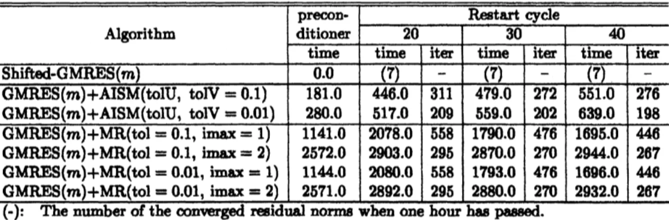
vector. ‘Itible1presents the$\infty mputation$time and

iteratians needed for satisfying thestoppingcriterion

$|\{r_{l}||_{2}/||b||_{2}<1.0x10^{-12}$ (10)

about $n$ the residualnorms, where $||r_{i}||_{2}$ is the i-th residual

nom

ofGMRES iterations. Tbe

value in brscket $u()$

means

the number of the raeidM

norms

that

can

not $\infty nverge$ within

one

1: select $c,$ $R,$ $N,$ $m$andvectors$b,$ $d$

2: set 吻$=c+R\alpha p(*j),$ $j=0,1,$$\ldots,$$N-1$ 3: solve $(A-\omega_{j}I)ae_{j}=b,$ $j=0,1,$$\ldots$,$N-1$

4: $M$ $f($_吻$)=d^{H_{l_{j}}},$ $j=0,1,$$\ldots,N-1$

5: compute $\beta_{j}=\pi^{1}\sum_{k=1}^{N-1}(w_{k}-e)^{j+1}f(w_{k}),$ $j=0,1,$

$\ldots,$$2m-1$ $6$: compute eigenvaiuee $\theta_{0},$

$\ldots,$ $\theta_{m}$of$ff_{m}-\lambda\overline{H}_{m}$ 7: compute $\lambda_{j}=\theta_{j}+c$

Figure 3. The algorithm to solve the eigenvalue problem with using tbe shifted linear$rnteI\infty$

‘Tlible 1. Example 1: Computation timeanditerations ofshifld $hnA$systems (time: computa.

tion time (s), iter: iterations)

$\infty nv\Re\Re$

.

Sme of theresidual norms

can

not $\infty nver\Re$ in

cases

ofMR method and the

Shifted-GMRES

$(m)$ algorithm. The mnputation time of MR preconditioner is much

more

expensive

than AISM $poeconditi\bm{m}\alpha$

,

and its cost is not practical. On the othoe hand, with uslng AISM

preeonditioner, the

iterations

are

termmated at mest threeminutes. Therefore,

we

find that it is

effectiveto aPply

one common

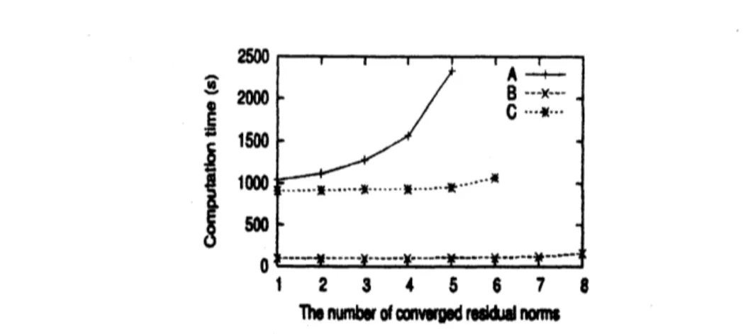
preconditionerto all thelinearsystems.

Figure 4 presents the number of the converged residual

norms

$u$ for the $\infty mputation$ time.

In the AISM method, all ofthe $\varpi idM$

norms

$\infty nvaege$ aimost $sim\iota \bm{P}\tan\infty mly$

.

In

case

of the

Shifld-GL4RES$(m)$ algorithm, the $\infty n\backslash \alpha genoe$ of the 5th residual

nom

i8 about 1,000 seeonds

slower than the hst \infty nwrg\’e residual

nom.

Also, it takes about 1,000 Kon& for the flrst

roeidd

mrm

to $\infty nv\alpha ae$

.

In MR $p\iota mnditior$, six residual

norms

$\infty nv\alpha ge$ almost the

same

time. However, tbe run time cost is about 1,000 seconds to $\infty nverge$, and the last tvve residual

norms

donot $\infty n\bm{v}eoe$

.

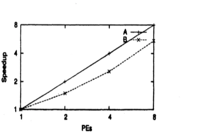
We

measure

the$pua\mathbb{I}el$perfiormanoe ofAISMmethod. In Figure5, uPto 4 PEs, tbe$\Phi^{\ovalbox{\tt\small REJECT} up}$

ratio isalmoet linear, and it is decreased in the

case

ofusing

8

PEs, andthe

sPeeduP

ratio isabout

4.5 tin$loe$

.

Rmple $l$] We $\infty n\mathfrak{g}ider$ tbe matrix, $nmdu_{ECL32’}$ in the Florida Sparse $Matr\dot{\alpha}$ 欧化 lleo

tion [6]. The order and

non

$ger\infty$ofthematrix

are

51,993, 347,007, respectively. Theright hand

side is determined

eo

that all theentries

are

1.0.

Just like in Example 1, the numberof shiftd

$\mathfrak{n}rnu\dagger ud\varpi m u\alpha dmi\hslash\ovalbox{\tt\small REJECT}$

Figure 4. Example 1: The relation of the number of converged residual

norms

and

$\infty mputation$ time ($A$: Shifted-GMRES(40), $B$: MR+GMRES(40), tol$=0.1$

,

IMAX$=1$

,

$C$:

AISM+GMRES(40), tolU, tolV$=0.1$)

Pb

Figure5. Example 1: Perfomanoeanslysisof

AISM

method, ($A$:idael, $B$: AISM method, tolU,

tolV$=0.1$)

3. In $th\dot{n}\alpha ample$

,

the oeIAral point of$c=(1.0,0)$ and tbe radius of$R=0.99$

are

selected.

Thble 2presents the$\infty mputation$timeanditerations needed for stoppingcriterion(10). Aceording

to this table, AISM method enable all the residual

norms

to converge about four

or

five times

faster than MR method. Also the preconditioningcostofAISMmethodisnot

so

expensive$u$ MR

method. Even if the iteratlom ofMRmethod “IMAX“ is increased, the$\infty mputation$eost

can

not

bereduoed, and rather$\alpha p\alpha 1$sive. The$c\infty t$ ofMR method ismore than 10 times

as

apansive _$u$

AISMmethod.

In the

Shifld-GMRES

$(m)a\Re rithm$

,

_{onlythelast reaidual}norm

can

_notconvergo. TherdOre,

we

analyze the relationbetween the $\infty nvoeffi$residual

norms

and$\infty mputation$time. Ftom Figure

6, the $\epsilon hiRd- GMhS(m)$ algorithm enables

seven

residual

norms

to ecmverge much faster than

tbe other $poe\infty ndition\ovalbox{\tt\small REJECT} GMR\bm{E}S(m)$ algorithm. However, the last

one can

not _{$\infty nver\Re$}

.

The

$Shifled- G\mapsto ms(m)$ algorithm is expensive for not all the linear systems, and the $\ovalbox{\tt\small REJECT}$ is

rather quick thanAISM metkd. Only

one

roeiduA

mrm

does not converge. Onthe otherhand,

$\mathbb{R}ble2$

.

Example2: Computation time and iteratiom of shifted linearsystms (time: _{$\infty mputa$}

.

tiontime (s), iter: $it\alpha atiom$)

lhenumber of oonvorgedresidualnerms

Figure 6. Example 2: The relation of the momber of Convergxl $r\alpha idM$

norms

and

$\infty mputation$ time ($A$

:

Shiftd-GMRES(20), $B$: MR+GMRES(20), tol_$=01$

,

IMAX$=1$

,

$C$:

AISM+GMRES(20), tolU, tolV$=0.1$)

Figure7shovva thespeedupratio ofAISM method. In this experinmot, the

_wallel

performanoe

is not

so

dffective

as

Example1, sinoethe gparse structureof the matrixis

more

irregular. In

case

of8 PEs, the speedup of about 4times isobtained.

6

Concluding

remarks

We have propoeed

a

new

technique ofAISM method for applying the shifted linear $\varphi tm$

.

In

the originalscheme, $eith\alpha$the Shifid-GMRES(m) algorithm without_{$pre\infty nditioning$}

or

the pae$\cdot$

eonditiCned

GMRES

$(m)$ algorithm with expensive$\infty mputation$ eoet, like MR method, is$\tau nu\triangleleft ly$

used. On the other hand, the proposed technique

can

$\infty mpute$

one common

$pr\infty ondition\alpha$of ffl

the systems. itdoes net depend

on

the momber of linear$\epsilon yst\epsilon m$

.

$Rom$two numerical rmples, it

iseffective to apply theAISM$proeonditi\bm{m}\varpi$to tbeshiftedlinearsystmswithusing tbe propoeed

technique. We

can

alsoobtain the speedup ratioofabout 4 timesby $u\epsilon ing8$ P&. Therebre, this

Pa

Figure 7. Example 2: Perfomanoe analysis of AISM method, ($A$

:

ideal, $B$: AISM, tolU,

tolV$=0.1$)

In the future work,

we

plan to study the detailed mmerical perfOrmamce of

our

algorithm to

allocating Aofshiftedsystms (2) toseed systm (1).

References

[1] GMRES: A Generalized Minilmal Residual Algorithm for Solving NonsymmetriC Lin$m$

Sys-tems, SIAM J Sci. Stat. Comput., No. 7, pp. 856-869 (1986).

[2] Ebommer, $A$, and Glassner,U.: naetarted GMRES $f\alpha$ Shifbed LinearSystems, SIAM J. Sci.

Comput., Vol. 19, pp. $1\succ 26$ (1998).

[3] Hudkel. T.: Appmimate Sparsity Patterns for the Inverse of

a

Matrix and Preeonditioning,

Appl. Numer. Math., No. 30, pp. $291-W\theta$ (1999).

[4] Bru, R., Crddn, J., and Marfn, J., Mas, J.: $Pr\infty Mition\dot{m}g$Spaise _{$Non\eta mmetric$} Lmm

systems with the $ShermaI\triangleright Morri8on$ Ebmula, $suM$ J.

Sci.

Comput., Vol. 25, No. 2, pp.

701-715

(2003).

[5] K. Moriya, L. Zhang, and T. Nodera: Tbe computation of the appmimate in$m$by

par-$a\mathbb{I}e\ ing$ tbe Sherman-Morrison fomula (in Japanese), J.

of

IPSJ, Vol. 48, No. 3 (2007) to

$appe\alpha$

.

[6] Unirsity of Florida Sparse Matrix Collection. [Online] http:$//www.ci\Re.\bm{t}.du/r/\epsilon p\sim$

$I^{I}ae/matri\infty$

.