Shallow ground water in the downstream basin of the Aya river, Kagawa prefecture. VI. On the characteristics of the belt of fluctuation of the water table during the period from October 1964 to September 1965-香川大学学術情報リポジトリ

(1)

（注意）この論文には正誤表があります

香川大学農学部学術報告第１９巻第１号正誤表 URL

http://www.lib.kagawa-u.ac.jp/metadb/up/AN00038339/AN00038339_19_1_e.pdf

Notice

Technical Bulletin of Faculty of Agriculture, Kagawa University Vol.19 No.1 Errata

URL

(2)

Vol 19, No 1 (1967)

SHALLOW GROUND WATER IN T H E DOWNSTREAM

BASIN

OF T H E AYA RIVER, KAGAWA PREFECTURE

VI On the Characteristics of' the Belt of' Fluctuation of' the Water

Table During the Period from October 1964 to September 1965

Kiyoshi FUKUDA, Katsuhiko Izursu, and Tadao MAEKAWA

B. Introduction

The belt of the fluctuation of the water table, or the belt of phreatic fluctuation is a part of the lithosphere and it lies a part of the time in the overlying zone of areation(l2). For our case of a shallow-ground water, the belt of the fluctuation of the water table is a zone between the water table at the highest stage('') and the lowest stage.('')

For a given region or aquifer, the volume of the belt of fluctuation of the water table is generally expressed in ha-m or area-depth.

By multiplying this volume of the belt by the specific yield, the net amount of ground water can be approximately calculated for a given region or aquifer during a specific period of rise or during a specified period of fall"

Therefore, it is important to find out the characteristics of the belt of the fluctuation of the water table in the study area.

The report presented here is the result of our study with the above objective using the data obtained from our field i n ~ e s t i ~ a t i o n s . ( l ' ~ ~ ~ ~ ~ ~ ~ ~ )

2. Notation AL : Left region, 139. 5 8 ha.

AR : Right region, 492. 8 5 ha.

Aw

: Whole study area, 632. 4 3 ha.

D d : The depth of the lowest stage of the water table or the deepest water table for the period from October 1964 to September 1965. The depth was measured from soil surface, m.

Ds

: T h e depth of the highest stage of the water table or the shallowest water table for the same period, m

A D : The difference between Dd and Ds or Dd-Ds (therefore Hd-Hs), m

d : Well depth measured from soil sureface, m .

H : Altitude of ground-surface, m.

H d : Altitude of the lowest stage of the water table or the deepest water table, m.

H g : Altitude of the well sites, m.

Hs : Altitude of the highest stage of the water table or the shallowest water table depth, m.

Ilrd: The gradient of Hd in the distance 1 I H ~ : The gradient of H g in the distance 1.

(3)

50 Tech. Bull. Fac Agr. Kagawa Univ.

IHS

: T h e gradient of

Hs

in the distance 1.

1

: Distance measured by 1/200000-topographic map, m.

M d :

Month having

Dd.

Ms

: Month having

Ds.

3.

Study

Procedures a. Study Area

As reported in the previous paper(7), the study area was divided into two regions; 1) the right region

AR

calculated as 492. 85 ha and 2) the left region, AL calculated as 139. 58 ha as shown in Fig. 1.

b. Longitudinal Water Table Profile T o make u p the longitudinal water table profile of the study area, we connected the observation wells along the Aya River irom the upper district to the lower district, and we made up six lines, R-1, R-2, R-3, R- 4, R-5 and R-6 for the right region, and four lines, L-1, L-2, L-3 and L-4 for the left region as shown by the solid lines in Fig. 1,

Fig 1 Study area and observation wells

c. Transversal Water Table Profile

T o make up the transversal water table profile of the study area, we conneced four observation wells, AR-1, AR-2, AR-4 and AR-6 in the right region, and we made up line AR as shown by the dotted line in Fig. 1.

Similarly, we made u p more five lines, BR, CR, DR, ER, and FR as shown in the same figure. For the left region, we also made up three lines, CL, DL, and E L as shown in the same figure.

4. Results

and

Discussion 4. 1. Values of'

Dd,

Ds,

and

AD

4. 1. 1. Va1ue.s of'

Dd,

Ds,

and

AD

From the data obtained from our field investigation, we made up Table 1 which shown the values of

Dd,

Ds,

AD

for the period from October 1964 to September 1965.

(4)

Vol. 19, No, 1 (1967) 5 1

Table 1. Values of Md, Dd, Mr, Dr, and AD

Well AR- 1 AR-2 AR-3 AR-4 AR-6 BR- 1 BR-2 BR-3 BR-4 BR- 5 BR-6 BR- 7 CR- 1 CR-2 CR-3 CR-4 CR- 5 CR-6 DR- I DR-2 DR-3 DR-4 DR- 5 DR-6 ER- I ER-2 ER-3 ER-4 ER- 5 FR- 1 FR-2 FR-3 FR-4 FR- 5 FR-6 BL-2 CL- 1 CL-2 CL-3 CL-4 DL- I DL-2 EL- 1 EL-2 EL-3 EL-4 FL- I DER- 1 DEL- 1 May 2 95 April 1 34 March, April 1 23 January 1 21 April 2 55 April 2 76 March, April 1. 71 January 1 18 April 1 38 January 1 65 February 0 82 May 2 85 June 2 73 April 1 99 April 1 40 Apr 11 1 36 April 1 58 August 1 33 March 1 59 February 1 70 April 1 46 March 1 24 January 1 01 March 2 66 March 1 08 April 1 27 January 1 58 January 1 35 February,March 2 14 January 1 16 Aprll 1 49 April 1 55 April 0 81 April 2 35 April 2 19 Aprll 2 89 January 2 54 April 1 85 April 1 56 April 1 15 April 2 17 March 1. 39 March 1 11 January 0 84 March 1. 16 May 1 09 March 2 09 March 1 43 April 2 06 September July .July September July, August August August September September September September September September August August, September July September September September July, August August July Septembel July July September June June, October September September July September September July ,June July August ,July, September August July September September July August September September September

(5)

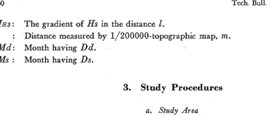
52 Tech. Bull.. Fac Agr.. Kagawa Univ.. From Table 1, we made up Table 2 which shows the concentration of M d and

Ms

during the period from October 1964 to September 1965.

Table 2 Concentration of Md and Mr

January February March April May June August Total 16 98 May 1 5 66 June 3 22 64 July 16 43 40 August 10 5 66 September 24 1 89 October 1 3 7 7 100 00 Total 55

There were 5 3 M d during the period from October 1964 to September 1965: 23 (43. 40 per cent) were in April, and 1 2 (22.64 per cent) were in March. Thus, 66.04 per cent occurred in the months of April and March. As a whole, the lowest stage of the water table or D d occurred in ~ ~ r i l ( ~ ) .

Similarly, Ms was concentrated in September (43.64 per cent) and July (29.09 per cent). Thus, as a whole, the highest stage of the water table or Ds occurred in ~ e ~ t e m b e r ( ~ ) .

b. Distribution of D d , Ds, and A D

Through the period fiom October 1964 to September 1965, the values of' D d varies from 0.81 m (FR-4 in April) to -2.95 m (AR-1 in May), Ds varies fiom 0..28 m (AR-4 in September) to 1.83 m (FL-1 in September), and A D varies from 0..22 m (FR-1) to 2.15 (BR-1) as listed on Table 3..

Table 3 Maximum and minimum values of Dd, Dr, and A D

Dd (m) D f (m) A D (m)

Max Min Max Min Max Min

-Value 2 95 0 81 1 83 0 28 2 15 0 22 Well AR- I FR-4 FL- 1 AR-4 BR- I FR- 1

Month May April September September

.4.. 1.. 2. Relation.ship between D d , Ds, A D , and d , and

Hg

a. Relationship between D d and

Hg

T o find out the relationship between D d and

H g

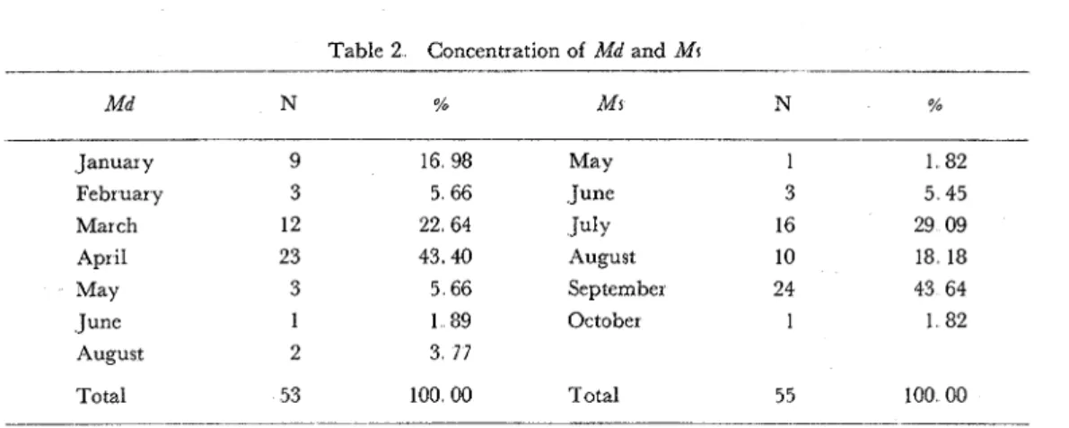
for the study area, we drew up three graphs as shown in Figs. 2-R (right region), 2-L (left region), and 2-W (the whole study area). The ,y-axes are the values of' the dependent variable D d , and the .x-axes are the independens variable

Hg.

(6)

Vol. 19, No 1 (1967) 53

Fig 2. Relationship between Dd and Hg.

There are various methods of determining the line which best fits the given points. W e used the one which is most widely used: the method of least squares(16).

In our case, for the data shown in Fig. 2 ( R , L, and W ) , the equation of the least-squares line is

and this can be found b y the values

and

a = ~ d - - a 2 2

(1.3).

Using Eqs.. (1.2) and (1.3), we calculated the data shown in Fig.. 2-R, and we calculated the values,

a=

- 0.0263, and a= 1.806. W e put these values into Eq. (1.1),

then we obtained Eq. (2). This is the line indicated in Fig. 2-R.

Similarly, from the data in Fig. 2-L, we obtained

a=

0.4332, and

a=

0.220,

and then we obtained Eq. ( 3 ) which is shown as the line in Fig.. 2-L.

Also from the data in Fig.. 2-W, we calculated the values,

a=

0..00696, and a= 1..640,

and then we obtained E q . ( 4 ) which is shown as the line in Fig. 2-W.

The results obtained from the calculation by using Eqs. ( 2 ) and ( 3 ) show that as the values of

Hg

increase frnm 0.0 to 6.0 m the values of D d decrease from 1.81 to 1.68 m in the right region whereas the values of D d increase from 0 22 to 2.82m in the left region.

(7)

54 Tech Bull Fac Agr, Kagawa Univ Using Eq. (4) for the whole study area, Dd increases from 1.64 to 1.68 m as

Hg

increases from 0.0 to 6.0m. These data are listed on Table 4.

Table 4 Calculated values of Dd, Ds, AD, and d

b. Relationship between D s and

Hg

Fig. 3 (R, L, and W) shows the relationship between D s and

Hg:

For the right region (Fig. 3-R), for the left region (Fig. 3-L), and for the whole study area (Fig. 3-W).

Fig 3 Relationship between D I and Hg

For the figures, the equation of the least-square line is

From the data in Fig. 3-R, we obtained

/3=

-0.0184 and b=0.911 by using Eq. (5), and then we made up Eq. (6). This is the line indicated in Fig. 3-R.

Similarly, we obtained Eq, (7) from Fig. 3-L, and Fq. (8) from Fig. 3-W. (Ds) L = 0.0878

H g

+

0.528 (7) (Ds)

w=

- 0.0105

Hg

$0.868 (8).

These are shown as the lines in Fig. 3-L and Fig. 3-W respectively.

The values of D s decrease slightly from 0.9 1 to 0.80 m as

Hg

increases from 0.0 to 6.0 m in the right region. The values of D s increase from 0.53 to 1.06 m in the left region. As a whole, D s decreases from 0.87 to 0.81m as

Hg

increases from 0.0 to 6.0m for the whole study area. These data are listed on Table 4.

(8)

Vol 19,No I (1967) 55

c. Relatzonship between A D and

Hg

Fig. 4 . Relationship between AD and Hg

For Fig. 4 ( R , L, and W ) which shows the relationship between A D and

Hg,

the equation of the least-square line is

Using Eq. ( 9 ) , we calculated the data in Fig. 4-R and we obtained Eq. ( l o ) , as shown by the line that is in the figure.

Similarly, from Fig. 2-L we obtained Eq. ( 1 1 ) as shown by the line in the figure, and Eq. (12) from Fig. 2-W

( A D )

w

= 0.0986Hg+ 0.394 _(12).

As

H g

increases from 0.0 to 6.0m, the values of A D increase from 0.38 to 0.93m in the right region and from - 0.31 to 1.77 m, in the left region.

As a whole, A D increases from 0 39 to 1,OOm as

Hg

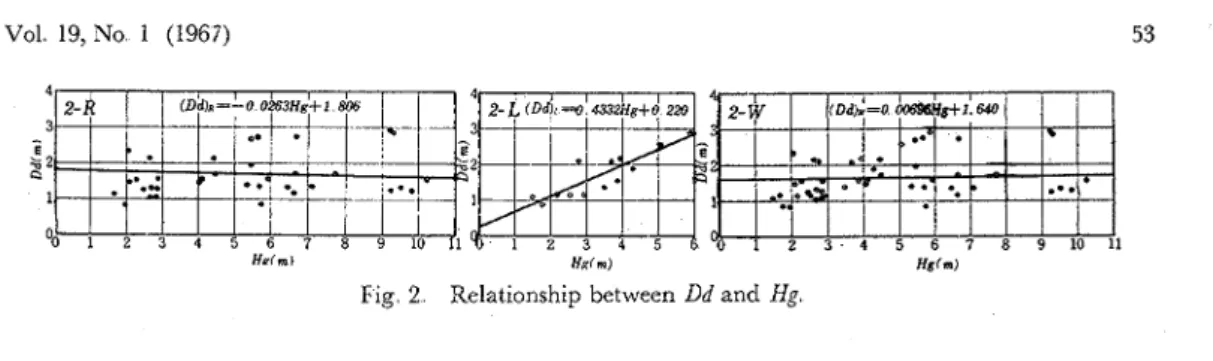
increase from 0 0 to 6.0 m for the whole study area. These data are listed on Table 4.

d. Relatzonship between d and

Hg

Fig 5 Relationship between d and Hg

Fig. 5 (R, L, and W) shows the relationship between d and

Hg,

For this figure, the equation of' the least-square line is

(9)

56 Tech Bull Eac Agr Kagawa Univ

- ---

H g d - H g d

I

6=

--2

H g 2 - %

and we obtained Eq. (14) fox the right region, and Eq. (15) for the left region and Eq. (16) for the whole study area.

As the values of

Hg

increase from 0.0 to 6.0 m, the values of d increase from 2.25 to 2.87m in the right region, from 1.31 to 3.72m in the left region, and from 2.19 t o 2.91m in the whoie study area. These data are listed on Table 4.

4. 2. Water Table Profile

4. 2. 1. Longitudinal Water Table Profile

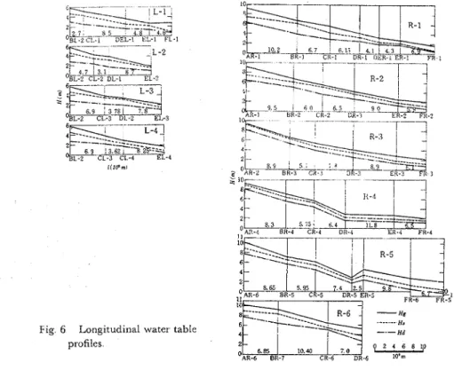
Fig. 6 shows the longitudinal water table profile of' the study area. In this figute, six graphs, R-1, R-2, R-3, R-4, R-5, and R-6, a r e of' the right region and four graphs, L-1,

._

I(1ff.J

Fig. 6 Longitudinal water table pr.ofiles

(10)

Vol 19,No 1 (1967)

L-2, L-3, and L-4, are of the left region (See Fig. 1).

a. Variation of

Hg, Hd, Hs,

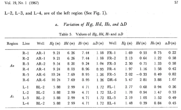
and AD Table 5 Values of Hg, Hd, Hr and A D

.- ---

Region Line Well Hg (m) Hd (m) Hr (m) AD (m) Well Ng (m) Hd (m) Hs (m) AD (m)

Rzght Regzon. From the graphs, R-1, R-2, R-3, R-4, R-5, and R-6, it is clear that the values of

Hg, Hd, Hs,

and AD decrease from the wells of the upper district's (on the left side of each graph) to the wells of the lower district's (on the right side of each graph). The values of

Hg

decrease from 9.21 -- 10.24 m to 1.69

-

5.74 m. The values of

Hd

decrease from 6.26 - 8.20 m to - 0 33 m (below sea level)

-

2.81 m, the values of

Hs

decrease from 7.44

-

9.24 m to 0.49

-

3.88 m, and AD decrease from 0.93

-

1.26 m to 0.22 - 1.07 m. These values are listcd on Table 5.

L e f t Regzon: As shown in graphs L-1, L-2, L-3, and L-4, the values of

Hg, Hd, Hs,

and

AD

decrease from the wells of the upper district to the wells of the lower district. The values of

Hg

decrease from 5 88m (BE-2) (on the right side of the graphs) to 1.48- 2.77m (on the left side of the graphs). The values of

Hd

decrease from 2.99m (BL-2) to 0.39-1.03 m the values of

Hs

decrease from 4.71 (BL-2) to 0.84-1.52 m, and the values of

AD decrease from 1.72 m (BE-2) to 0.26 - 0.53 m. These data are listed on Table 5. b.. Variation of

IH g, I H

d , and

IHS

TO see if the line of'

Hs

is parallel to the line of'

Hd

in Fig. 6, we introduced the following thr.ee equations ;

(18), and

(11)

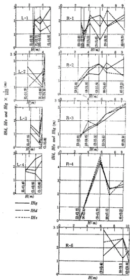
58 Tech Bull Fac Agr Kagawa Univ in Fig. 6, and the results are shown in Fig. 7.

Fig. 7 also shows the relationship between k g , I H ~ , and

IHS.

Five graphs, R-1, R-2, R-3, R-4, and R-6 are for the right region, and four graphs, L-1, L-2, L-3, and L-4 are for the left region.

As shown in Fig. 6 (line R-1), line H s is not parallel with either line Hd or line H g : thus, line I H ~ , I H ~ , and

IHS

are not parallel as shown in Fig. 7 (R-1). As shown in Fig. 1 , line R-1 runs along the right side of the Aya River, thus, the variations are influenced by the river. The water level of the river fluctuates greatly in the irrigation period, therefore line H d , the lowcst stage of the water table, does not parallel line Hs, the highest stage of the water table, whereas line Hd is parallel to line H g , (the altitude of the well sites) as shown in Fig. 7 (R-1).

Graph R-2 shows that three lines, I H ~ , I H ~ , and IHS, are roughly parallel to each other. As shown in Fig. 1, R-2 is further away from the Aya River than line R-1. Therefore, the influence of the river on the water table is smaller.

Graph Pi-3 and R-4 show that I H ~ , I H ~ , and

IHS

are parallel to each other As shown in Fig. 1 , lines R-3 and R-4 run through the middle of the right region from the upper to the lowcr districts, thus, the influence of the river is very small. From the shape of the two lines,

HfmJ

Flg 7 Relationsh~p between IHd, IHr, and R-3 and R-4 shown in Fig. 7, the following are IHe

-

made clear : 1 ) the water table at the highest stage is parallel to the ground-surface, 2) the water table at the lowest stage is also parallel to the ground-surface, and 3) the gradient of H g , H d , and Hs or I H ~ , I H ~ , and

IHS

decrease roughly as the altitude of ground surface of

H

decreases.

c. Variation of D d , Ds, and A D and

Hg

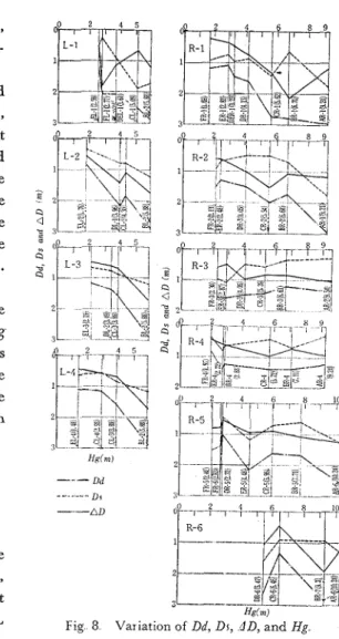
Fig. 8 shows the variation of D d , Ds, and A D and

Hg

for the period from October 1 9 6 4 to September 1965. Graphs R-1, R-2, R-3, R-4, R-5, and R-6 are for the right region, and L-1, L-2, L-3, and L-4 are for the left region.

Rzght Region: In graph R-3, the value of A D is about 1,0 m between AR-2

(Hg=

9 . 5 4 m ) and DR-3 (Hg=4.05m). In graph R-4, the value of A D is also about 1.0m between AR-4

(12)

Vol 19, No 1 (1967) 59

district to the middle district (See line DR), the values of AD are roughly 1.0 m every- where.

Between wells ER-3

(Hg=

2.87 m ) and FR-3 (Hg=2.30 m) shown in graph R-3, the values of

AD

are about 0.5m. And at the two wells ER-4 ( H g 2 . 7 2 m) and FR-4 ( H g = 1.97 m), the values of

AD

are

also 0.5m. Wells on lines ER and FR are

'

distributed over the lower district or the

region and most of them are along the coast of the Inland Sea as shown in Fig. 1.

L e f t Regzon: In graph L-3, the value of AD is about 0.5m between CL-3

( f i g

= 3.89 m) and EL-4

(Hg=

1.48 m). Wells CL-3, CL-4, DL-3, EL-2, and EL-4 are in the rice fields of the region near the coast of the Inland Sea as shown in Fig. 1.

4. 2. 2 T r a n ~ v e r s a l W a t e r T a b l e P r o j l e -.

-

Dd

-- -. DI

-AD

a. Va7zatzon of H g , H d , and

HS

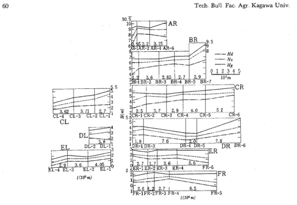
Fig. 9 shows the transversal water table profile of the study area. Six graphs AR, BR, CR, DR, ER, and FR are for the right

Hsirn)

region and three graphs CL, DL, and E L _Fig₈ _Var~atlon_{of Dd,}_Dr,_4D,_and_Hg are for the left region.

Rzght regzon: In the three graphs, AR, BR, and CR, the values of

Hg

decrease from right side to the left side of the figure. The right side corresponds to the district near the mountain and the left side to the district close to the Aya River as shown in Fig. 1.

In the two graphs, BR, and CR,

Hd

and H s decrease from the mountain side to the river side. T h e shallow ground-water in this part goes into the Aya River. The Aya River in this part is effluent stream(13) with respect to the shallow ground-water

In the graph DR, lines H g , Hd and

HS

form a valley at two wells, DR-4 and DR-5, in the middle of this water table profile.

From this, in this part of the region, the shallow ground-water goes into the Kamidant River as shown in Fig. 1. This was inferred from the contour lines of the study area made up in the f i r d 2 ) and the third reports(6) of this study. Also, from thc two graphs, E R a n d FR, the shallow ground-water goes into the Kamidani River.

According to the two contour-line maps shown in the third report (one based on the irrigation period average and the other based on the non-irrigation) the contour lines are similar in shape, thus, the shaiiow ground-water of this area goes into the Kamidani River through-

(13)

Tech Bull Fac Agr Kagawa Univ

Fig 9 Transversal water table profiles

out the year The Kamidani River in this area is effluent stream with respect to the shallow ground-water

L e f t Regzon: On all of the graphs, CL, DL, and EL, the values of H g decrease from the right side to the left side, The right side is the river side and the left side is the sea side as shown in Fig 1. The profiles of H d , and Hs also decline from the river side to the sea side.

b. Variation of D d , Ds, and A D

Fig. 10 shows thc variation of D d , Ds, and A D on the transversal water table profile of the study area. Six graphs, AR, BR, CR, DR, ER, and FR are for the right region, and three graphs, CL, DL, and E L are for the left region.

R i g h t Region : The values of D d decrease from the profile AR to profile FR D d decreases from the upper district to the lower district of the region. On the other hand, the values of Ds increase from the profile AR to profile FR, thatis Ds increases from the upper district to the lower district. Thus, the values of A D or Dd-Ds, decrease from the upper district to the lower district.

From profile AR to profile CR, the values of A D are about 1 Om below the ground surface whereas they are about 0.5 m below the ground surface from piofile DR to profile FR.

As shown in Fig. 1, the three profiles, AR, BR, and CR, are in the upper part of the right region, and the rest, DR, ER, and FR, are in the lower part of the region : thus, differences between the highest and the lowest stages of the water table ( = A D ) are about 1.0m in the upper region and 0.5 m in the lower.

The large values of D d , and

Ds

occur along the areas near the riper and the mountains. Wells AR-6, BR-7, DR-6, and ER-5 are located along the mountain range and the values

(14)

Vol 19, No 1 (1967)

Fig 10 Variation of Dd, Dr, and 4 D

of D , and Ds in these wells are large. Wells AR-1, BR-1, and CR-1 are located along the right side of the Aya River, and well FR-6 is located near the left side of the Kamidani River, thus, the values of D d , and Ds in these wells are large.

However, the values of D d and Ds are small in wells DR-1, ER-1, and FR-1 although these wells are located along the right side of the Aya River This is due to the fact that the water flows into the river in this area(14).

Left Regzon: Three graphs, CL, DL, and E L show that the wells located on the river side have large values of D d and AD. In graph EL, the values of D d , Ds, and A D are roughly constant; D d is about 1 Om, Ds and A D are about 0.5m. Wells on the profile are located on the lower part of the region (near the coast of the Inland Sea as shown in Fig. 1).

5. Summary

T o find out the characteristics of the belt of fluctuation of the water table during the period from October 1964 to September 1965, we made u p the longitudinal and transversal profiles of the water table of the study area by using the data obtained from our field investigations, The method we used and the results of the study are as follows:

T o find out the relationship between D d and

Hg,

we used the Least-Squares Method and we obtained three linear equations; Eqo (2) for the right region, Eq. (3) for the left region, and Eq. (4) for the whole study area. The result of the calculation was that the values of D d increased from 1 6 4 to 1 6 8 m as the values of

Hg

increased from 0 0 to 6.0m in the whole study area.

Similarly, we obtained three linear equations, Eqs. (6), (7), a n d (8), to see the relationship between Ds and

H g

Using these equations we found that the values of Ds decreased from 0.87 to 0.81 m as the values of

Hg

increased from 0 0 to 6.0 m in the whole study area.

For the values of A D and

Hg,

we obtained Eqs. ( l o ) , (ll), and (12) Using these equations we found that the values of A D increased from 0.39 to 1.00 m as the values of

Hg

(15)

62 Tech Bull Fac Agr Kagawa Univ

For the values of

d

and

Hg,

we formulated three equations Eqs. (14), (15), and (16). Using these equations we found that the values of

d

increased from 2.19 to 2.91 m as the values

H g

increased from 0.0 to 6.0 m in the whole study area.

As shown in Fig. 1 , we made u p ten longitudinal lines of the study area connecting wells, R-1, R-2, R-3, R-4, R-5, and R-6 for the right region and L-1, L-2, L-3, and L-4 for the left region. Following these lines, we made up ten longitudinal profiles for each of the following water tables,

D d , Ds,

and

A D

as shown in Fig. 6.

W e also made u p nine transversal lines of the study arca connecting the wells as shown in Fig. 1 , AR, BR, CR, DR, ER, and FR for the right region and CL, DL, and E L for the left region. Following these lines, we made up nine transversal profiles for each of the following water tables,

D d , Ds

and

A D

as shown in Fig. 9.

The lowest stage of the water tables occurred 5 3 times in seven months of which 43.40 per cent occurred in April. The shallowest stage of the water tables occurred 5 5 times in six months of which 43. 6 4 per cent occurred in September.

T h e maximum value of the lowest stage of the water tables was 2.95m (AR-1, May) and the minimum value was 0 8 1 m (FR-4 April). For the shallowest stage of the water tables, they were 1.83m FL-1, September) and 0.28m (AR-4, September), and for the distance between the lowest and the shallowest stages, they were 2.15m (BR-1) and 0.22m (FR-1).

T h e writers wish to thank Former Professor Dr. Hitoshi FUIWDA, and Associate Professor Dr. Hiroyuki OGATA both of Tokyo University for their encouragement.

A part of expenditure was from the research fund donated by the Ministry of Education.

References

(1) FUKUDA, K , OCHI, T , KONO, Y , SHIIKI, K , NARUHIRO, 'ISHIMONO, , S : Shallow-Ground Water in the Downstream Basin of the Aya River, I, Tech Bull Fac Agr Kagawa U n z u , 17, 29-35 (1965)

(2) FUKUDA, K , OCHI, T , I ~ O N O , Y

,

MAEKAWA, T , SHIIKI, K , NARUHIRO, T , SHIMONO, S :

zbzd, 11, 32 (1965)

(3) FUKUDA, K ,NAGANO, T ,OCHI , T , MAEKAWA, T : Shallow-Ground Water in the Down- stream Basin of the Aya River, 111, T e ~ h Bull Fac Agr Kagawa Unzv

,

18, 54-65 (1966)

(4) FUKUDA, K , NAGANO, T ,OCHI, T

,

MAEKAWA, T : t b z d , 18, 60 (1966)

(5) FUKUDA, K , NAGANO, T , &HI, T

,

MAEKAWA, T : t b z d , 18, 60 (1966)

(6) FUKUDA, K , NAGANO, T , &HI, T, MAEKAWA, T : tbzd, 18, 63-64 (1966)

(7) FUKUDA, K , NAGANO, T , MAEKAWA, T : Shallow-Ground Water in the Downstream Basin of the Aya River, IV, Tech Bull Fac

Agr Kagawa Unto 1 8 , 186-187 (1967)

(8) FUKUDA, K

,

NAGANO, 'I, MAEKAWA, T :

zbtd, 18, 186-207 (1967)

(9) FUKUDA, K : Shallow-Ground Water in the Downstream Basin of the Aya River, V, Tech

Bull Fa6 Agr Kagawa Unto ,18,208-209 (1967).

(10) MEINZER, 0 E : Outline of Ground-Water Hydrology, 35, Government Printing Office, Washington (1923)

(1 1) MEINZER, 0 E : zbtd , 35 (12) MEINZER, 0 E : t b t d , 35-36 (13) MEINZER, 0 E : zbzd, 56 (14) ~ / I E I X Z E R , 0 E : t b t d , 56

(1 5) OCHI, T

,

FUKUDA, K

,

AOKI, 7 : Shallow- Ground Water in the Downstream Basin of the 4ya River, 11, Tech Bull Fac Agr Kagawa

Untu

,

17, 42-49 (1965)

(16) W A S H I I L G ~ O ~ , A : Basic Technical Mathe- matics with Calculus, 330-331, Addison- Wesley Publishing Co , Inc

,

London (1965)

(16)

Vol. 19, No 1 (1967)

Ql1l-F

%%a

tz

8 tlf-

b

&E&'F'7k

VI 1 9 6 4 + 1 o ~ ; s ~ 1 ; 1 9 6 5 q 9 a t ~ ~ a r ~ ~ 1 2 k a i r . a j . v a Belt of' fluctuation D@@i'C-> l l '-C

Belt of fluctuation dj 5 l rid: Belt of phreatic fluctuation it Lithosphere ~ - - 2 $ T d j 5 hr, Z D6JfRTd2, Z.&% Dd (BR&7;7JUW.) t: Dr (@g&T7j~{$,) ~ f i i j ~ ? $ * t : L?:,, 5 2. h & f i & @ o Belt of fluctuation DgCb, --,&CZ, i l i j @ i % F d t @ T Z S h 6 ,, L?:;t)r,7T, ZD%9.B%.%6 Z k l t , e ~ % @ D . & l i & ' T 7 k % . i i m c z ~ ~ ~ - g - , j 2 , b z + . a r a l 9 g . % . x 6 . ,

e

ZT1964@10fl->1965@9 a ~ g R B u B e t C z & t : ~ + t > - c g t f i g , % + . 7:. $ 6 # l . g ~ f ? i i 4 4 C z Z ~ & i ' d . ~ ~ ~ & j T d j 5 . 1) $ T , Dd, Dr, .4D (= Dd- Dr) 3

sit

20 ( ~5tlfi1.. Dd C;4 0 81-2. 95772, Dr it 0. 28-1 83m,

e

L T AD 12 0 22-2. 15m

2,

h>7Ld (3 D E l a . Z f - (Table 3)., 2) 9 + C t , Dd

t:

D r h l X % T 5 8 l t , 2~8;t,l. Dd it 1, 2, 3, 4, .5, 6 B k i 3 8 a ~ 7 ~ E l i c h 7 : , 7 T X % T 6 h r , % a 4 3 40%Ct 4alZffZb&5.. Dr i t , 5, 6, 7, 8, 9 B d r U ; l O f l l ~ b f : ~ T X % T 6 h 1 : , 9 f l , Z i t , +%D43. 64%;bf1Yi5?, LTL > 6 (Table 2),,

3) Dd, Dr, AD %& U; d (@&lijft-$~@S) fil Hg (N,+.D@&) @ @ ( L ~ L # ~ J ,7T 2 j E&$5 $3. Dd

&@$& Hg B.&HK