Shallow-ground water in the downstream basin of the Aya river, Kagawa prefecture (5) On the characteristics of the cumulated depth-area curve and depth-area curve (I)-香川大学学術情報リポジトリ

Tech Bull Fac. A ~ I Kagawa Univ

SHALLOW

-

GROUND WATER IN THE DOWNSTREAM BASIN

O F THE AYA RIVER, KAGAWA PREFECTURE

(5)

ON THE CHARACTERISTICS OF THE CUMULATED DEPTH-AREA CURVE AND DEPTH-AREA CURVE

( 1 )

Ki yoshi FUKUDA

Introduction

In the previous paper,(') we drew up isobath maps for every month of a phreatic cycle from October 1964 to September 1965, and from these maps we were able to see the layout of the water table of the drainage basin from the beginning of the non-irrigation to the irrigation period.

From the studies concerning the isobath maps, we obtained t h e curves showing the relationship between the depth of the water table and its corresponding area. These curves are refered to as the Depth-Area Curve, or more simply, the D-A Curve of the study ar ea

.

I t is very important to know the D-A Curve to know the hydrological characteristics of a drainage basin, Each drainage basin has its own D-A Curve.

For practical purposes we often encountered the need to know the water-table depth for a given area for a given month. For example, to plan a n irrigation and drainage project, we need to know how large of an area occupied by 0.5 nz or less depth in September (the phreatic high of the study area). This information will also give us something to base further projects on. Thus, the Depth-Area Curve is useful.

This paper reports the construction, the characteristics, and the possible use of the D-A Curve

Method Study Area

As reported i n the psevious paper,") the study area was divided into the two regions; 1) the right region, and 2) the left region of the Aya River a s shown in Fig.. 1, and we call them the right region and the left region respectively Fig. 1 The study area. hereafter. The area of the right region,

Vol. 18, No. 2 (1 967) 209

AR (ha), was calculated as 492.85 ha, and the area of the left region, AL (ha), a s

157.94 ha.(2) The whole study area, the sum of the right region and the left region, Aw

(ha), is obtained as follows;

Aw=AR t AL

AR =492.85 ha, AL =157.94 ha, and Aw =650.79 ha.

.. .

₍₁₎

Classifying of the Water -Table Depth

In the previous paper, the range of the water-table depth fluctuation was shown from 0.5 m or less to 3.5 rn, and the range was divided into seven classes with a 0.5 m-interval. The classification mas used to draw up the isotath maps shown in Fig. 1 to Fig. 15 in the previous paper(" and it mas used to make up the Depth- Area Curve, D. A. C

,

shown in Fig. 3-A, Fig. 3-B, and Fig. 3-C in this paper. However, to draw up the Cumulated Depth- Area Curve, C. D. A.C., as shown in Fig. 4 (A to 0)

,

the water -table depth must be reclassified into another seven- classes, the cumulated - seven classes that i s general1 y used for making a summation curve in statistics.

The data from Table 1(4) of the previous paper were used for the Depth- Area Curve, and the Cumulated Depth- Area Curve.

Results and Discussion Variation of the Water -Table Depth

Average Depth, Dav

Statistics tells us that the arithmetic average of the various depth of the water table for a given drainage basin is simply given by the following equation;

n

C a

where a l , a e ,

.

-,an represents the area having Dl, D z , , Dn respectively,

D l , D 2 , , , Dn represents the depth of the water table classed into n-classes with a class- interval.

Because the water-table depth was classed into seven classes, in Eq. (2) , n=7. Thus, the average depth of the water table in the right region, D a v ~ (m), is obtained by the

following equation; I

CUR

D

D a v ~ =---

.

" .

AR (3)

where LZR represents an area (ha) of the seven-classes water-table depth, D(m), and AR represents the area of the right region or 492.85 ha.

Similarly, Eq. (4) for the left region, and Eq. (5) for the whole study area were obtained.

7

where Dav~ represents the average water-table depth of the left region, U L represents an area (ha) having a seven-classes depth, D (m), and

21 0 Tech Bull Fac Agr Kagawa Univ and where Davwrepresents the average water-table depth of the whole study area, m ,

aw represents an area having a seven-classes depth, D ( m ) , and

A w

represents the area of the whole study area ( h a ) or 650.79 ha.

Using Eqs. ( 3 , ( 4 , and (5), the data listed on Table were computed and the values of D a v ~ , D a v ~

,

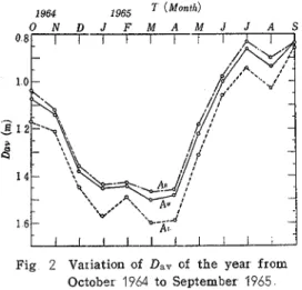
and Davw for every month from October 1964 to September 1965 were obtained as shown in the three curves in Fig. 2. The chain-line shows the variation of Dav of the right region, the dotted line for the left region, and the full line for the whole study area.

Fig. 2 also shows the variation of Dav~

,

1964 1965 7 (Month)

O N D J F M A M J J A S Dav~

,

and Davw of the year Values of Dav

m

vary from 1 47 m (March) to 0 83 rn (July)

in the right region and they vary from 1 6 0 m (March) to 0.86 m (September) in the left region, and for the whole study area, Dav vary from 1 . 5 0 ~ ~ (March) to 0 . 8 4 ~ ~ (Sep- tember). The yearly average of Dav are 1 17 m (the right region), 1 . 2 7 ~ ~ (the left region), and I 17 m (the whole study area). (The curves resemble that of the curves@) in Fig 2 Variation of Dav of the year from the previous paper

.

)

Octob~r 1964 to September 1965 The periodical average of Dav are 0.89 m (the right region), 0.97 m (the left region), and 0.91 rn (the whole study area) for the irrigation period aod they are 1 ..31 rn (the right region), 1.41 rn (the left region), and 1.34 m (the whole study area) for the non-irrigation period

During the low stage of the phreatic cycle from January to April, the values of Dav are small. They are from 1.60m to 1.,47m.

During the high stage of the phreatic cycle from July to September, the values of Dav are relatively high, from 1.03m to 0.83 m..

The average values of Dav in the high stage are 0.86 m for the right region, 0.,94 m for the left region, and 0.88 m for the whole study area and they are 1 .,45 rn for the right region, 1.56m for the left region, and 1 . 4 7 ~ ~ for the whole study area in the low stage.

The period from the low stage to the high stage is called the period of risecQ)-May and ,June.. In this period, the water-table depth gets shallower as shown in Fig, 2.. The period from the high stage to the low stage is called the period of de~line(~~)-October, November, and December.. In this period, the water-table depth gets deeper a s shown in Fig. 2. Thus, the values of Dav decrease from 1

..

04 m to 1 "45 m ..

The values of Dav in the shallowest water-table depth, or in the phreatic high, are 0.83 m (the right region in ,July)

,

0.86 m (the left region in September), and 0.84 m (the whole study area in September) ; and in the deepest, or the phreatic low, they are 1 '.47 m

(the right region in March), 1.60 m (the left ,region in March), and 1 m (the whole study area in March). These data are listed on Table 1 .

The valley on the curve i n Fig. 2 for Table 1 The values of Day

August in 1965 shows the effect of the Dav ( m )

irrigation cut off of several days (this is Period

AIE Ale, Aw

done to strengthen the roots of the rice

plants). The water table decline and the average 1 17 1 27 1 17 valley on the curve appeared, as shown in Periodical average

Fig.. 2.

Our report corresponds to the Nelson's

Irrigation 089 0 9 7 091

Non-irrigation 1 31 1 41 1 34 Stage average

repor t(12) where the phreatic high occurred

High stage 0 86 0 94 0 88 in July in 1922, June in 1923, and August

L O W stage 1 45 1 56 1 47

in 1924; and the phreatic low occurred in

Phreatic values

March in 1922, April in 1923, and March Phreatic high O 83 O 86 O 84 in 1924. Nelson's report was conducted in (July) (Sept (Sept

1 47 1 60 1 50 the Egin Benchof Snake River Plain, Idaho, _- Phreatic low (March) (March) (March) and he drew up a figure showing the An: The right region

annual manipulation of the Egin water table AL : The left region

A w : The whole study area through an irrigation season. The curve in

his figure was much the same as our Fig. 2 From Nelson's figure, we obtained the values of the depth of the water table at the phreatic high and low. They were four feet (July 1923), five feet (June 1923), and 3.6 feet (August 1924) for the phreatic high, and 24 feet (March 1922), 23.5 feet (April 1923) and 25 feet (March 1924) for the phreatic low. The only difference between the two figures was the valley on the curve of the phreatic high in August in Fig. 2.

However, the curve on Fig. 2 is in reverse to the Meinzer's report("). Meinzer's report shows the phreatic high to be between February and April and the phreatic low to be between August and September. Meinzer drew up a figure showing the fluctuation of the water table at Jones ranch, Big Smoky Valley, Nev From this figure, we obtained the values of the depth of the water table at the phreatic high and low. For the phreatic high, they were 7.6 feet (between February and March, 1914), 7.4 feet (between March and April, 1915), and 7.3 feet (between February and March, 1916), and for the phreatic low, they were 9 feet (between September and October 1913), 10 feet (between August and September in 1 9 1 4 , and 10 8 feet (between August and September in 1915).

Modal D e p t h , Drnode

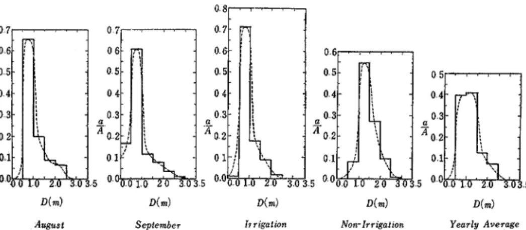
From the data on Table I('), we drew up Figures 3-A, 3-B, and 3-C showing the

a

relationship between the water-table depth, D ( m ) , and the area ---- for every month.. A

The abscissa is D (m) and the ordinate is Fig. 3-A shows the Depth-Area Curve of the right region, Fig.. 3-B for the left region, and Fig

..

3-C for the whole study area.

The full line on the graph is the "histogram" of the distribution of the water-table depth,

D

(m), and the curve on the graph is the "frequency curve" of

D

(m). As is defined in statistics, the most often recurring score is the mode, and is general, the mode

Tech. Bull., Fac. Agr .. Kagawa Univ,.

October November December January February

Fig 3-A Depth-Area Curve of the right region (Octobel 1964 to February 1965)

October November December January Februavy

Eig 3-B Depth-Area Curve of the left region (October 1964 to February 1965)

October Norember December lanaary February

Fig 3-C Depth-Area Curve of the whole study area (October 1964 to February 1965)

M a r c h Aprrl May June July Fig 3-A Depth-Area Curve of the right region

(March to July in 1965)

D(m) D(m) D(m) D(m) D(m)

March Aprzl May June July

Fig 3-B Depth-area Curve of the right region (March to July in 1965)

March A p r i l May .June July

Fig 3-C Depth-Area Curve of the whole study area (March to .July in 1965)

Tech. Bull. Fac. Agr Kagawa Univ

Augus: september IT? tgat ron Norr ITT tgat ton Yearly Average Fig 3-A Depth-Area Curve of the right region

(August and September in 1965, and the irr igation,non .ir I igation, and the yearly average)

August September I~rigation Non-Irrigation Yearly Average Fig 3-B Depth-Area Curve of the left region

(August and September in 1965, and the irrigation, non-irrigation, and the yearly average)

Aug~rsl September I?rrgatron Noa-Irrrgatron Yearly Average Fig. 3-C Depth-Area Curve of the whole study area

(August and September In 1965, and the irrigation, non-ir r igation and the yearly average )

v o l . 18, No. 2 (1967) 21 5

tells us just where in the data a concentration of measures exist.

Therefore, the mode of the graphs is the water -table depth which occurred largest area in a given month. We refere to the water-table depth corresponding to the mode, as the "modal water. table depth" or " D m o d e " , and the class corresponding to the mode, "modal

water -table class" or "DCmod,".

The shape of the Depth- Area Curve influences the median (discussed in the next section) and average depth of the water table. The same depth of the same median may in two widely differing type of distribution. In fact, there is an infinite variety of the Depth- Area Curve for a given median or average depth. Therefore, the parameter other than the median or average are necessary to define a Depth-Area Curve. One of the parameter is the mode.

The curves shown in Fig. 3-A, Fig. 3-B, and Fig. 3-C show the mono-modal distribution a

curves; and from these curves, we obtained the values of D m o d e , D C m o d e and -- A for every

a

month, and the result is listed on Table 2. The values of are shown in the decimal fractions in Fig. 3-A, Fig. 3-B, and Fig. 3-C, but they are shown in percentage on Table

a

2. The values of - corresponding to D m o d e = I .25 m are listed and outlined on Table 2.

A

Table 2 T h e values of Dm,,de and

+-

Month D C m o d e D m o d e - D m o d e D m o d e A ( m ) ( m ) (%> ( m ) (%) (m)

(%I

October 1964 05-10 075

1

5601 125 41241 0.75 5187 November December Januar y February March April May June July August September AE : T h e right region AL : The left region. Aw: The whole study area

In the right region, D m o d e is 1.25 m during the five months from December to April and

a

the values of - decrease from 74,,30 (December) to 63.17 (February), however, D r n o d e

A

a

is 0 . 7 5 ~ ~ during the seven-month from May to November and increases from 39.36 A

21 6 Tech Bull. Fac Agr

.

Kagawa Univ In the left region, during the four months from June to September or the irrigation

a

period, Drnode is 0 75 m, and -

A increases f rom 48.67 (June) to 68.98 (July)

,

but during a

the non-irrigation period, D m o d e i s 1.25 m and increases from 41.24 (October) to 58.32

(January)

.

As for the whole study area, from December to May D r n o d e is 1.25 m; and in the

remaining six months, D m o d e is 0.75 m. Therefore, over half of the study area is occu-

pied by 0.5 to 1 .O m-depth of 1.0 to 1.5 m-depth of the water table except for November and May. In these two months, they occupy around 40 per cent.

Mediale Depth, D m e d

From the data listed on Table 1c4), we also drew up Fig. 4 (A to 0 ) . Every figure on Fig. 4 has three curves; 1) the curve shown by the chain-line for the right region, 2 ) the curve shown by the dotted line for the left region, and 3) the curve shown by the full line for the whole study area. These curves are also called ogives that were introduced into statistics by Sir Francis GaltoncB).

1 0 a 0 8 8 , a r a

,

r , ,

*);

-<;;,-

+ - ~ ~ ~ P - y' -

-

- November

-

1 9 6 4

-

Aw

-

- -

An

-

..-.--- AL

-

- , I , , , , l , , , , l , , , , f * ; 1 5 2 0 2 5 3 0 D ( m ) D ( m )

Fig. 4-A Cumulated Depth- Area Curve Fig 4-B Cumulated Depth -A1 ea CUI ve

of October

,

1964 of November, 1964

D ( m ) D ( m )

Fig. 4-C Cumulated Depth-Area C u ~ v e Fig, 4-D Cumulated Depth-Area Curve

D ( m ) D ( m )

Fig 4-E Cumulated Depth-Area Curve Fig 4-F Cumulated Depth- Area Curve of Feb~uar y

,

1965 of M a ~ c h , 1965.

D ( m ) D ( m )

Fig. 4-G Cumulated Depth-Area Curve Fig 4-H Cumulated Depth- Ar ea Curve

of April, 1965 of May, 1965

D ( m ) D ( m )

F!g 4-1 Cumulated Depth-Area Curve Fig. 4-J Cumulatad Depth- Area Curve

Tech. Bull Fac Agr Kagawa Uaiv

D ( m ) D ( m )

Fig 4-K Cumulated Depth-Area Curve Fig 4-L Cumulated Depth- Area Curve

of August, 1965 of September, 1965

o

Irrigation Per iod D ( m )

A w

-

Non-Irr igation D ( m )

Fig.4-M Cumulated Depth- Area Curve Fig 4-N Cumulated Depth-Area Curve of the irrigation period of the non-irrigation period

O O ~ , , I W ~ , 1110, r i i i , , I , , , , r I I ! I I I I ,

, j

/

0 0 0 5 1 0 1 5 2 0 2 5 3 0

Yearly Average D ( m )

Fig. 4-0 Cumulated Depth-Area Curve of the yearly average.

The curves shown in Fig. 4-A to Fig. 4-L tell us the relationship between the cumulated water-table depth and the area of the right and left regions and the whole study area for every month of the year from October 1964 to September 1 9 6 5 Fig. 4-M shows the relationship between the cumulated water-table depth asd the area for the irrigation period, Fig.

4-N

for the non-irrigation period, and F i g .

4-0

for the yearly average.

From the curve shown in Fig. 4 (A to L), we obtained the values of 0 5 0 , the water- table depth occupying 50 per cent of the study area for every month of the year, and the results are shown in Fig .5.

As is defined in statistics, the mid point

r

( M o n t h ) 1964 1965

of a series of number is called the median. O N D J F M A M J J A S

a 0 4

In our case, D50 is the mid point of the A

axis having the values from 0.0 to 1.0 in Fig. 4 (A to 0 ) . D50 was defined as the

water -table depth occupying 50 per cent of the study area that is, D50 corresponding to

a

the value of ----=0.5, Therefore, we refere A

to Dso as the "median 'depth" or "Dmed"

1 2 hereafter

.

The vlaues of the depth corresponding 25 _Lu--l

-per cent of the study area or D25, and 75 Fig 5 Variation of Dmea of t h e year from

October 1964 to September 1965 percent or D75 also are obtained from F i g . 4

(A to 0 ) and the evaluation for every month is shown in Fig.

6

(A, B, and C).

a

25 per cent is one fourth of 100 per cent of --- -axis in Fig.

4

(A to 0 )

,

thus, we A T (Month) 1964 1965 O N D J F M A M J J A T (Month) 1964 1965 O N D J F M A M J J A S T ( M o n t h )

Fig 6-A Variation of 0 2 6 , D S O , and Dr6 for the right region of the year from October 1964 to Septem- ber 1965

Fig 6-B Variation of D 2 5 , D S 0 , and D76 for the left region of the year from October 1964 to Sep- tember 1965

Fig 6-C Variation of DB6, D S O , and Dr6 for the whole study aIea of the year from October 1964 to September 1965

220 Tech. Bull. Fac. Agr. Kagawa Univ. refere to Dz5 as the first quartile depth of the water -table depth or Dlq, similarly, D75 as the third quartile depth or D3q hereafter.

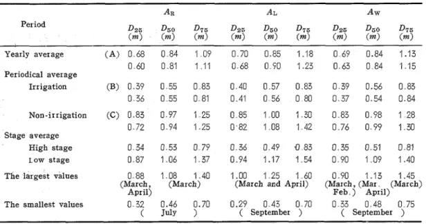
The values of 025, D50r and D75 for the irrigation period and non-irrigation period, and the yearly average are also obtained from Fig. 4-M, Fig. 4-N, and Fig. 4-0 respectively and are listed on Table 3.

Table 3 The values of D25, DSO, and D7&

Period

Yearly average Periodical average

Irrigation

Non -ir r igation Stage average

High stage

LOW stage

The largest values

The smallest values

( A ) 0 68 0 84 1 09 0 6 0 0 8 1 1 1 1 (B) 0 39 0 55 0 83 0 36 0 55 0 81 (C) 0 83 0 97 1 25 0 72 0 94 1 25 0 8 8 1 . 0 8 1 . 4 0 (March, (March) April) 0.32 0.46 0.70 ( July ) 1.00 1 2 5 1 6 0

(March and April)

0.29 0 . 4 3 0.70

( September )

0 . 9 0 1.13 1.45

(March, (Mar (March) F e b . ) April)

0 3 3 0 . 4 8 0 7 5

( September ) (A) : Figures obtained from the isobath map based on the yearly average (Fig 4-0)

(B) : Figures obtained from the isobath map based on the periodical average, irrigation, (Fig 4-M) (C) : Figures obtained from the isobath map based on the periodical average, non-irrigation,

(Fig 4-N)

AR : The right region AL : The left region Aw: The whole study area

T h e values of Dmed fluctuate frcm 0.43 m (the left region in September) to 1.25m (the left region in March and April). The yearly average is around 0.84 m. During the irrigation period, Dmad is around 0.56 m and it decrease to 0.98 m during the non-irrigation period. In the high stage, Dmed is around 0.51 m and it declines to around 1.09 m in the low stage. These data are listed on Table 3.

To obtain the values of DL5, D50 or Dmed, and D75 of the yearly average, we used two methods; 1) by the simple arithmetic average of the data obtained from 12 isobath maps of the year from October 1964 to September 1965-Method I, and 2) by the data from the yearly-average-isobath map drawn from the data of the 12 isobath maps of the same year -Method 2.

I n Table 3, the figures obtained from Method 2 are listed on line (A). Similarly, to obtain the values of D25, D50 or Dmed and D75 for the periodical average (both the irrigation and non-irrigation), we used the two methods. Figures listed on line (B) and

(C) are the figures obtained by Method 2.

The figures obtained from the two methods are very similar to each other for the yearly and periodical average.

The water-table depth occupying 25 per cent of the study area, D25, fluctuates from 0.29 (the left region in September) to 1.00 m (the left region in March) through the year, and its yearly average is around 0 69 m (the whole study area). The periodical average

of 0 7 5 varies from 0 . 3 9 ~ ~ in the irrigation perisd to 0.85 m in the non-irrigation period.

At the high stage, DZ5 is 0.35m (the whole study area) and it declines to 0.9Om (the whole study area) a t the low stage These data are listed on Dz5-column on Table 3.

075, the water table depth occupying three fourth of the study area fluctuates in the range from 0.70 m (the right region in July and the left region in September) to 1.60 m (the left region in March and April)

.

The yearly average of D75 is around 1 .I5 m (the whole study area).

For the irr igation-per iod average, D75 IS 0.83 m and for the non-irr igation period, it is

around 1.28 m (the whole study area). The average for the high stage, D75 is around 0.81 m (the whole study area) and for the low stage it is 1.4Om (the whole study area). These data are listed on column of D75 on Table 3.

As a whole, in the greater part of the whole study area, the water table fluctuates in the range from n.75 m ( in September) to 1.45 m (in March), however, a fourth of the area goes from 0.33 m (in September) to 0.90 m (in March and February)

.

Half of the whole study area, the water table ranges from 0 . 4 8 ~ ~ (in September) to 1 13 m (in March and April)

.

Uniformity of the Water -Table Depth CoeflfY cient o f Uni:fbrmit,y, f'

An expression for measuring uniformity which depends on the ratio of areas above and below the '50 per cent line in a summation curve of grain-size distribution is called Kramer's uniformity modulus('). We applied this Kramer's modulus to our study a s a parameter defining the uniformity of the distribution of the water-table depth. We refere to f as the coefficient of uniformity of the water-table depth, and it is defined by the

*following equation;

where A represents the area above 50 per cent line of the curve shown in Fig. 7 , and

B represents th2 area below the line. In Fig. 7, it is evident geometrically that f' has two typical values depending ..on the shape of the Cumulated Depth- Area-Curve ; they are 1 ) when D (m) is uniform or in the water- table depth equals

222 Tech. Bull

.

Fac.. Agr

.

Kagawa Univ. Depth-Area Curve is the straight line that is parallel to ,y-axis at D= 1.0 m as shown by the dotted line, and area A equals area B, thus, , f = l .

2) when D (m) is uniform distribution, the Cumulated Depth-Area Curve is the straight

a

line connecting the two points, one point having T=O and D = 0 m, and the other point a

having

T =

1.0 and D=3.25 m as shown by the chain-line, and area B is one third of I

area A, thus, f

=-.

3

To get area A and area B for every curve of Fig.

4

(A to 0 )

,

every curve was traced on a Imm-mesh-tracing paper and the area was computed by the mesh-counting method, and the values of f were obtained by using Eq. (6).

The results of the calculation using the above equation is shown in Fig. 8.

The values of f vary from 0.270 (the left region in September) to 0.660 (the right region in December), and yearly average is around 0.583 (the whole study area). During the irrigation period, f is around 0.439 (the

whole study area) whereas it is 0.611 (the

whole study area) during the non-irrigation Table 4 The values of f period.

These data are listed on Table 4.

B f=- Period A AR AL Aw lo[ I A I I I 1 - 1 Yearlyavexage 0 603 0 547 0 583

3

Periodical average Irrigation 0 443 0 410 0 439 Non-irrigation - 0 616 0 602 0 611 Stage average High stage 0 391 0 366 0 376 f L O W stage 0 604 0 561 0 593

The largest values 0 660 0 598 0 631 (Dec ) (April) (Dec )

1

The smallest values 0 358 0 270 0 363 (Aug.1 (Sept ) (Aug )

0 0

0

P, : The area above the 50 per cent line o f a

O N D J F M A M J J A S A

1964 I965 in F'ig 4 (A to 0 )

B : The area below of the line T (Month)

A R : The right region Fig 8 Variation of f of the year f ~ o m AL : The left region

October 1964 t o September 1965 Aw: The whole study area

1

To calculate the deviation of f from the values of f = I and f=---, the following 3

equation was used;

f

f =(----I) x100(%)

"

.

. . . .

f s

.

(7)

where crf represents the deviation of f from f

,

f represents the coefficient of the uniformity having the particular values of

1) f s = 1

,

when the water -table depth is uniform, and

2) f s=-- .when the water-table depth is uniform distribution (See Fig. 7), and

Vol. 18, No. 2 (1967) 223

,f represents the coefficient of uniformity of the water-table depth shown in Fig. 7 and on Table 4.

The evaluation using the above equation is shown in Figs. 9-A, 9-B, and 9-C.

In Fig. 9-A, Fig. 9-B, and Fig. 9-C, the curves of f never coincide with x-axis or r t =0,

thus, the distribution of the water-table depth is, here again, neither in uniform nor in uniform distribution for both regions through the year.

'

..-.,'

"',

a

I L L l L l l O N D J F M A M J J A S , f g 6 f D j g 6 5 F M A M J J A S 1964 1965 , t A L L L L L u y g 6 ! D J F M A M J J A S 1965

T (Month) T (Month) T (Month)

Fig 9-A Variationon of af for Fig 9-B Variation of a* for Fig 9-C Variation of or for the

the light region the left region. whole study area

However, the shape of the Depth- Area Curve shown in Fig. 3 tells us the curves are the skewed depth distribution curves with mono-modal depth having 0.5 to

I .Om-depth or 1.0

to 1.5 m-depth. This modal depth occupied over half of the study area through the year. Therefore, over half of the study area is in uniform depth with 0.5 to 1 "0 m-depth or 1 .U

to 1.5 m-depth depending on the month.

Quartile Deviatzons, Qa

,

Qg

,

and logQg

There are three kinds of quartile deviations that are used for determing the deviation of the grain-size dist~ibution(~). We applied them to our case as the parameters defining the deviation of the uniformity of the water -table depth of the study area, thus, we refere to following equations as the parameters ;

1) Arithmetic q u ~ tile deviation, &a

Q . =

+

( D ~ ~ - D ~ ~ )

.

,

.

, , , , , ,

.

, ,

.

,

.

, ,

.

, , ,, , ,, , , ,,

.

,, , , (8) 2 ) Geometric quartile deviation, Qg

3) Log

-

quartile deviation, logQg 1

log&, =-(l0gD3q -20gDlq)

.

2

UO)

where D3q represents the water-table depth occupying 75 per cent of the study area or

D,75, and

Dlq represents the water-table depth occupying 25 per cent of the study area or 0 2 5

-

224 Tech. Bull Fac Agr Kagawa Univ the study area, thus, the following values are obtained by Eqs. (8), ( 9 , and (1 O),

Qa =0, Q B = I , and logQg =O

. . . . . . .

(11).

. D3q=Dla

When the water-table depth is in uniform distribution, 0"9=3, the values of Qg and Dl4

log&, are obtained as follows;

Qg = 1.732, and, ZogQg =0.2385 I

Because of the values of Qa vary with the limit-depth of the water table or the deepest water -table depth, we do not use Qa hereafter

.

(see Fig

.

10)

.

From Fig.

4

(A to O), the values of D3q or D75 and Dlq or DZ5 for both regions (AR and

A L ) of every month are obtained, and the values of Qg and logQg are calculated by Eqs. (9) and (1 0) respectively, and the results are shown in Fig. 11 and Fig. 13.

Fig. 11 shows the variation of Qg of the year. In this figure, line Qg =I .732 shows that the water-table depth is in uniform, and line Qg =1.0 or x-axis shows that the water- table depth is in uniform distribution. The curve shows the water-table depth in the study area is neither in uniform nor in uni- form distribution,

To calculate the deviation of Qg from Qgs, we used the following equation,

Q

aQg = (L-l)

x

100

(%)

..

"

.

(13)

Qgs

where oQg represents the deviation of Qg from Qgs,

Qg represents the geometric deviation

D (d defined by Eq

.

(9) , and

Fig 10

Qgs represents Qg having particular values of 1) Qgs= 1 .732 when the water-table depth is in uniform distribution as defined by Eq.

1 6 (12) and, 2) Qgs=l when the

water -table depth is in uniform as defined by Eq. (11).

The result of the calculation using the above equations are shown in Fig. 12-A for the .-

right region, Fig. 12-B for the left region.

1 0 1 1 1 1 1 1 1 1 1 1

O N D J F M A M J J A S When Qgs=l .732, the values of oQgs are

1964 1965 below the 30 per cent line whereas they are

T (Month) above the line when Qgs=l

.

From December

. .

AR : The right region.. _{to April, the values of cQg of Qg =I .732} AL : The left region.

Fig. 11 Variation of Q, for the right and and Qgs=l are about the same 30 per cent. left regions. Therefore, the water-table depth of the study

area is in neither uniform nor in uniform distribution. however, it is closer to the uniform distribution. From the shape of the curve, shown in Fig. 3 ( A , B, and C ) , the depth is closer to the uniform rather than the uniform distribution.

O N D J F M A M J J A S 1964 1965 T (Month) 60 0 1 l l l l l l l l l l l O N D J F M A M J J A S 1964 1965 T (Month)

Fig 12-A(above) Variation of cQg for the right region.

Fig. 12-B (below) Variation of cQg for the left region

0 0

0 N D J F M . A M J J A S

1964 1965 T (Month) AR : The right region. AL : The left region.

Fig.. 13 Variation of log&, for the right and left regions.

Fig. 13 shows the variation of log-quartile deviation or log&, of the year. In this figure line, log&, =O. 2385 shows that the water -table

depth is in uniform distribution, and line

log&, =O or x-axis is in uniform. The curve do not coincide with the lines, thus, the water -table depth in the study area is neither in uniform nor in uniform distribution.

Using Eq. ( I d ) , the deviation of log&, from

logQ,s are obtained, and the results are shown

in Fig. 14-A for the right region and Fig. 14-B for the left region.

O N D J F M A M J J A S 1964 1965 T (Month) 100 &---*---4.---+---Q----+ ---+- 80 _{log Qgs} ---%--_--- _=o 1 O N D J F M A M J J A S 1964 1965 T (Month)

Fig,, 14-A(above) Variation of c log&, fo.1 the right region

Fig. 14-B (below) Variation of clog&, for the left region.

log&

clog&, = ( Z . - l ) x 100(') ..,,

....

...

...

. .

.

....

. ,,.

....

l0gQgs , ,

.

(14)

The values of clog&, are about the 80 per cent line in both graphs when logQgs=O, however, when logQ,~=0.2385, the values of clog&, are below the 60 per cent line.

226 Tech Bull Fac Agr. Kagawa Univ I n the right region when logQgs=0.2385. The values of ologQg are below the 30 per cent line from May to November, however ,the values are above 90 per cent from December to April. Therefore, the water -table depth in this study area is neither in uniform distribution nor in uniform. However, in the right region from December t o April the depth is closer to the rather uniform than the uniform distribution.

As a whole, from the shape of the curves shown in Figs. 9-A, 9-B, and 9-C; and Figs. 12-A, and 12-B; and Figs. 14-A, and 14-B, the water--table depth in the study area is neither in uniform nor i n uniform distribution. However, from May to November, the water-table depth is closer to the uniform distribution: From December to April, the depth is closer to the uniform.

According to the curves shown in Fig. 3 (A, B, and C)

,

over half of the study area are occupied by a water-table depth of 0.5 to 1.0 m-depth or 1.0 to 1.5 m-depth depending on the month, therefore, the depth in over half of the study area is in uniform with 0.5 to 1

.O

m-depth or 1.0 to 1.5 m-depth.

Summary

From the isobath maps shown in the previous paper, we drew up the Cumulated Depth- Area Curve and the Depth-Area Curve of the right region, left region, and the whole study area for the year from October 1964 to September 1965. The characteristics of these curves were studied and the result was as follows;

1)

As the parameter defining the depth of the water table of the study area, we used three kinds af parameters; 1) Average depth, Dav, 2) Modal depth, D m o d e , and 3) Median depth,

D m e d

.

1) Average depth, Dav was defined by the following equation; n

Dav = C ( a D ) , n=7, where a represents the area having D , and D, the depth of the n

C a

water table classified into n-class (in this study, n=J) with a class interval. For the whole study area, the values of Dav varied from 1.50 m (March) to 0.84 m (September) and the yearly average was obtained as 1.17m. We also obtained the values of D a v a s 0.91 m for the i~rigation-period average and 1.34m for the non-irrigation period

2) The modal depth, D m o d e , was defined as the depth which occupied the largest area of

the study area in a given month. The values of D m o d e was obtained from Fig. 4 (A to 0 )

as 0 5 to 1

.O

m-depth or 1 0 to 1.5 m-depth. Over half of the right and left regions were occupied with the modal depth of 0.5 to 1 .O m-depth or 1 0 to 1.5 m-depth depending on the month.

3) In the Cumulated Depth-Area Curve, Fig. 4 (A to O), the depth occupying 25 per cent of the study area was ref er ed to D25. Similar 1 y

,

we obtained D50 and D75. D50 was also refered to as the median depth, D m e d . The values of these parameters were obtained a s

follows

D m e d fluctuated from 0.43 m to 1.25 m through the year, and the yearly average was 0.84 m. D25 varied from 0.29 m to 1.00 m through the year and the yearly average was

Vol. 18, No. 2 (1967) 227 0.69 m. D75 was 0.70 m for the shallowest and 1.60 m for the deepest values for the year, and it was 1.13 m for the yearly average.

The curves showing the variation of D25, 050, 0 7 5 , and Dav resembled and paralleled to

one another in Figs. 6-A, 6-B, and 6-C.

2)

To study the uniformity of the water-table depth of the study area, coefficient of uniformity, f , and the three kinds of quartile deviation, Qa

,

Qg

,

and log&, were defined

1) Appliying Kramer's modulus, we refered to as the coefficient of uniformity, f is defined as following equation;

B

f =- A

,

where A represents the area above the 50 per cent line of the Cumulated Depth- Area Curve shown in Fig 4 (A to O), and B, the area below the line.

The values of f were 0.270 to 0.660 through the year, thus, the water-table depth of the study area is neither i n uniform nor i n uniform distribution, because f = 1 is uniform

1

and f =---- is uniform distribution. 3

The three kinds of the quartile deviation were defined in the following equations. Arithmetic quartile deviation, Qa = - - l - ( ~ 3 q - ~ i q ) ,

2.

Geometric quartile deviation, Qg =

(a)+,

and Dla

Log-quartile deviation, logQg = L ( : Z O ~ D ~ ~ - L ~ ~ D ~ ~ ) , 2

where D3q was the third quartile depth or D75, and Dlq was the first quartile depth or D25. When the water-table depth is in uniform, Qa =O, Qg =I, and logQg =0, and when the depth is in uniform distribution, Qg =I "732, and log&, =0.2385. And &a is not constant but variable, varying with the limit-depth.

The result obtained from these equations shows that the water -table depth is neither in uniform nor in uniform distribution through the year. However, from the shape of the curve shown in Figs. 9-A, 9-B, and 9--C, and Figs. 12-A, and 12-B, and Figs 14-A, and 14-B, the water-table depth is closer to the uniform distribution for the months from May to November. From December to April, the depth is closer to the uniform.

From the curve shown in Figs 3-A, 3-B, and 3-C, over half of the study area were occupied by 0.5 to 1 .O m-depth or 1.0 to 1.5 m-depth. Therefore, over half of the study area was in uniform depth through the year

Acknowledgments

The writer wish to thank Professor Hitoshi FUKUDA, Assistant Professor Hiroyuki OGATA both of Tokyo University for their encouragement. Also Assistant Professor Shigemi TAKAYAMA of Rissho University for his suggestion concerning this study. The help of Mrs. Chieko MATSUBARA in making the culculation, charts, and figures, is greatfully acknowl- edged. A part of expenditure was defrayed by the research fund donated by the Ministry of Education.

228 T e c h . Bull Fac Agr Kagawa Univ

References

(1) FUKUDA K . , NAGANO T

,

and MAEKAWA T . : sha, Tokyo

Tech Bull Fac A g r Kaqawa Unrv., 18 (7) KRAMER H : Trans A S C. E. 100, 798-

186-207 (1 966) 838: sited by DALLAVALLE J M . : Micromerztics,

(2) FUKUDA K

,

NAGANO T . , and MAEKAWA T : Second Edition, 58-59, (1948), Pitman Publishing

Tech Bull Fac Agr K a g a w a Unzv., 18 Corporation, New York

187 (1966) (8) KUBO K

,

MIZUWATARI E

,

NAKAGAWA Y

(3) FUKUDA K

,

NAGANO T

,

and MAEKAWA T : and HAYAKAWA S Funtai, 80-81

,

(1 964),

Tech. Bull F a c Agr Kagawa Unzv

,

I 8 Maruzen, Tokyo

190-202(1966). (9) MEINZER E : Ouflzne of Ground- Water Hydro-

(4) FUKUDA K

,

NAGANO T

,

and MAEKAWA T : l o g y , 34-36 (1923), Government Pxinting Office,

7ech Bull Fac A g r Kagawa Univ., I 8 Washington,

188-189 (1 961) (I@ MEINER 0 E : -34-35-

(5) FUKUDA K

,

NAGANO T . , and MAEKAWA T : U1) MEINZER 0 E : -36-.

Tech Bull. F a c Agr Kagawa Univ

,

18 60 (12) NELSON H. : Report f o r drscussion Questzon

(1 966) 17, 128, Fifth Congress on Irrigation and Drain.

(6) Galton F : sited by Kenkyu-sha's New Eng- a g e , Tokyo-1 963

l i s h - Japanese Dzcttonar y , 1245 (1963) Kenkyu-

Cumulated Depth- Area Curve % U\' Depth- Area Curve D ~ J E K Q L . -C

(1)

3-

83

B

~ S W D

Isobath map b, Cumulated Depth-Area Curve, C D A C % 1 U' Depth- Area Curve, D A . C & f s k C D A . C % & u \ ' D A C D y - u M + , x-@MD (m) &s$r5i, D (m) Mf&sr5'bafl7 ki&T7k@, m , a M&%D D (m) %@?Ei@, ha; $31 U' A L;f. (id?&) i&%a3+E+B7 ha, T d j 6

C D A C % & U.'D A C M, - Q D R ~ & K ~ C . ~ L , -9B% 6 , Drainage basin ~ f & 7 ; / k t $ ~ & 3 2 ~ B ( J @ ~ & ? 3 $ % S k % k b i % 6

+$A D D A C K % L . -c, + s ~ k . l i E & @ ~ D (m) D@,% (0 0-3 5m D P ~ B , 0 5m ZU+ K 7 E f i ) & M o d a l Class, DCmode; Modal depth p D m o d e t: L k D C modo M, 0 5-1 Om, Ad: U.' 1 0-1 5m 0 2 %,%;5i

th%

L ,

% D & ~ ~ ; f j ~ H , 0 5-0 6 C & Z DCmcde M, fi&AiSSL\BK, E b \ Demode MI % a \ h f i i b \ B K .%hi% 6

@9

x,

L D i & R T H , B+, 50-60%DG&5, % DJJ K k Q -C, 0 5-1 Om d j 6 L\M, 1 0-: 5m ~ i f F 7 k @ ~

E % ~ ~ ~ L K Z E S ~ % Z L \ ~

C D A C

a,

D (m) @OgiveT+,dj.fj D (m) di, + D f & i $ T u n i f o r m K & 6 D f i ~ , d j b L \ H , uniform

B

distribution K dj 6 Dfibez-j- parameter t: L

r ,

Coefficient of uniformity, f = X & % A L ~ A a C D A C.

0+=0 5 1 OkD%fiDEi%, B M M L < ~ ; D % ~ D B % P & &

1

D (m) ~ i u n i f o r m ~ t : $ ~ , f = l ; uniform distributionDt:$H, f = ~ , T d j & a i , C D i & f & D f M, 1 2 1

Vol. 18, No. 2 (1967)

D ( m )

a

uniformity %$Jz-j-6glJa parameter 2 L T , 3 @ a Quartile deviation % G A L 7?:

I

1) Arithmetic quartile deviation: &a=- ₂ (Daq-Dlq),

'2) Geometric quartile deviation : Q ~ = ( & )

',

f 1 G

D l ,

3) ~ o g - q u a r t i l e deviation: log Q , = L (log Dsq-log Dl,) Ds,

a

third quartile depth (=D75), Dlq 2

M first quartile depth (=D25) Tibj 6

D ( m ) f3: uniform 2

$?a,

&a= 0 , Qg= 1

,

$+ 1 U; l o g Q g = 0 ; $ k D ( m ) f 3 j uniform distribution 0 tr

P a , Qg= I 732 $+ 1 h l o g Qg=O 2385 % % 3 6 (&a tt constant 2 ?'s: b f K D ((m a a k U ~ # ; i a ~ -C @%jli-b-6)

25, Z ~f&@i~ Q a , Q g , f l h log Qg a7 I S Z % i i & O b \ T ; h k & - & L k L \

z a f & i & a D ( m )

a ,

~ 7 7 % u n i f o r m T & , uniform d i s t r i b u t i o n ~ & k ~ ~ L ~ J ~ L ~ - I I J ~ O & . ~ ~ ~ % K

L O % < , 1 2 - 4 ) ? j ~ & J j M , m $ K d : ! J % b \ DCmodet D m o d e 0 . ) ~ ~ f 3 ~ % % % S k T L \ 6 ~ 2 % % $

Z D G f % K H , *%%HYRR??

(@zmf.R.

fifi3) D @ @ % % V k %Bk%bj-