Title: Bifurcation and stabilization of oscillations in ring neural networks with inertia Authors: Yo Horikawa, Hiroyuki Kitajima
Affiliation: Faculty of Engineering, Kagawa University, Takamatsu, 761-0396, Japan Corresponding author:
Yo Horikawa
Faculty of Engineering, Kagawa University, Takamatsu, 761-0396, Japan Phone: +81-87-864-2211
Fax: +81-87-864-2262
E-mail address: [email protected]
Abstract:
Effects of inertia on oscillations in ring networks of unidirectionally coupled sigmoidal neurons are studied. It is known that ring neural networks without inertia are bistable and the duration of transient oscillations increases exponentially with the number of neurons. In this paper, kinematical description of traveling waves in the oscillations in the networks is extended to networks with inertia. When inertia is below a critical value and the state of each neuron is over damped, properties of the networks are qualitatively the same as those without inertia. The duration of the transient oscillations then increases with inertia, and the increasing rate of the logarithm of the duration becomes more than double. When inertia exceeds a critical value and the state of each neuron becomes under damped, properties of the networks qualitatively change. The periodic solution is then stabilized through the pitchfork bifurcation as inertia increases. More bifurcations occur so that various periodic solutions are generated, and the stability of the periodic solutions changes alternately. Further, stable oscillations generated with inertia are observed in an experiment on an analog circuit.
PACS codes:
05.40.-a, 05.45.-a, 87.19lj
Keywords: Ring neural network; Inertia; Traveling wave; Kinematical model; Bifurcation
Selected Classifications 60: Dynamical systems 185: Neuroscience
205: Non-linear waves and stability 210: Oscillatory dynamics
1. Introduction
Ring networks of neurons are of wide interest in physiological and biological modeling [1 and references therein] since they cause various spatiotemporal patterns, and they are used as models of central pattern generators in the nervous systems for instance [2]. The asymptotic properties of ring networks of unidirectionally coupled neurons with sigmoidal output functions are simple [3 - 6] although it is known that discretization [7] and delays [8 - 12] cause complicated behaviors. Their stable states are of three kinds depending on the gains of the output functions and couplings of neurons. When coupling gains are small, the origin, at which the states of all neurons are zero, is a globally stable state. When coupling gains exceed threshold values, the origin becomes unstable. Then they show stable oscillations generated through the Hopf bifurcations if the numbers of inhibitory couplings are odd, which are qualitatively the same as ring oscillators [13]. On the other hand, the networks become globally bistable through the pitchfork bifurcations if the numbers of inhibitory couplings are even. The bistable states of neurons are symmetric with respect to the origin, i.e. ±xp. There are also periodic solutions showing oscillations in the states of neurons, but they are unstable and the networks reach one of the bistable states eventually.
Recently, however, it was shown that oscillations during transition to the steady states in the bistable networks last extremely long time in computer simulation [14 - 16] and experiments on an analog circuit [17]. It was then shown that the duration of the transient oscillations increases exponentially with the number of neurons [18, 19]. The periodic solutions and transient oscillations are traveling waves rotating in the network, in which neurons are divided in two blocks, and the signs of their states are positive in one block and negative in the other block. The boundaries of the blocks then propagate in the direction of couplings, e.g. (+, +, +, -, -, -, -, -) → (-, +, +, +, -, -, -, -) → (-, -, +, +, +, -, -, -) ···. The states of neurons change their signs when the boundaries pass so that they oscillate. In the periodic solutions, the numbers of neurons in two blocks are the same. Kinematics of the traveling boundaries has shown that the velocities of the boundaries increase as the numbers of neurons in the forward blocks decrease. The number of neurons in a block including a smaller number of neurons (the length of a smaller block) then decreases and finally the boundaries of the block collide and the block disappears. The oscillation then ceases and the network reaches one of the steady states. However, difference in the velocities of the boundaries is exponentially small with the numbers of neurons in the blocks so that the oscillations last exponentially long.
These exponential increases in the transient oscillations mean that, when the numbers of neurons are large, the networks never reach their asymptotically stable steady states in observation time and the transient oscillations are stable in practice. Such exponential dependence of transient time on system size has been found in a one-dimensional reaction-diffusion equation [20 - 23], in which the motion of fronts and kinks is extremely slow and transient patterns last exponentially long with the length of a domain. Further, it has been shown that the duration of various transient patterns in higher-dimensional reaction-diffusion systems shows exponential dependence on system size, which is called metastable dynamics [24, 25 and references therein]. Exponentially long transient states have also been found in complicated patterns including transient chaos in coupled map lattices [26], reaction-diffusion equations [27] and neural networks [28 - 30]. These metastable dynamics and exponential transients are of wide interest.
Diffusive couplings are generally used for connection and interaction between neurons. However, it is known that inertia has considerable effects on properties of coupled dynamical systems. It causes complicated response of coupled sigmoidal neurons. Two neurons coupled both resistively and inductively show chaotic response to external forces [10, 31], and two-neuron systems with one inertial term exhibit chaos [32]. Finite frequency response of
neurons due to conduction delays of signals also has effects equivalent to inertial couplings [10]. From viewpoints of artificial neural networks, it is well known that back propagation learning can be accelerated and escape from local minima is enabled by adding momentum terms [33]. In general, all physical components in electronic circuits contain some inherent inductance. Response of nerve membrane in the resting state shows the existence of phenomenological inductance in itself [34]. Dynamical neuron models such as the BVP (Bonhoeffer-van der Pol) model, which generate impulses and show spontaneous firing, contain inductance in their analog circuits [35, 36].
Further, collective synchronization in coupled oscillator systems with inertia has been extensively studied in various fields [37 - 39]. In the context of nervous systems, synchronized firing in populations of fireflies of a certain species was explained by adding frequency adaptation as well as phase, which leads to a system of the second-order differential equations [40]. Effects of inertia were also examined on phase resetting and desynchronization in spontaneous firing of neurons with a two-dimensional phase oscillator model [41], which was physiologically derived with interaction between axons and dendrites [42]. In addition, in the field of electronics engineering, it has been shown that nonlinear oscillators coupled with inductance exhibit various synchronization, bifurcation and chaotic patterns [43 - 45].
What inertia causes in periodic solutions and transient oscillations in the unidirectionally coupled bistable ring neural networks is thus of interest. As mentioned above, they are two traveling boundaries of two blocks of neurons rotating in the network. The velocity of each boundary depends on the number of neurons in the forward block. This dependence results from the relaxation process of the states of neurons. The state of each neuron approaches one of the steady states, and the approaching state changes as the boundary passes. The velocity of the boundary is large when the absolute value of the state of a neuron at the passage time of the boundary is small. In the absence of inertia, changes in the states of neurons are described with the first-order differential equations, and their approach to the steady states is monotonic and exponential. The monotonicity causes the instability of periodic solutions, and the exponentiality causes exponentially long transient oscillations. In the presence of inertia, however, changes in the states of neurons are described with the second-order differential equations, and their recovery process to the steady states can be under damped (damped oscillatory). This oscillatory relaxation of the states of neurons due to inertia is then expected to change the stability of periodic solutions. In this paper, we derive a kinematical equation of the traveling boundaries in the networks in the presence of inertia. Using the kinematics, we first show that the increasing rate of the duration of the transient oscillations with the number of neurons increases with inertia in an over damping mode. Next, it is shown that inertia causes the pitchfork bifurcations of periodic solutions and stabilizes oscillations in an under damping mode. Further, it is shown that successive bifurcations make asymmetric periodic solutions and periodic solutions of higher harmonics stable. These qualitative changes in the properties of the networks and the coexistence of oscillations of various patterns caused by inertia are of interest.
The rest of the paper is organized as follows. In Sect. 2, a model of the ring neural network with inertial terms is explained and its solutions of traveling wave type and spatiotemporal patterns of the states of neurons are shown with computer simulation. In Sect. 3, kinematical description of the traveling waves in the network is derived. In Sect. 4, it is shown that the duration of the transient oscillations increases and the periodic solutions are stabilized owing to inertia. Stable oscillations observed in an experiment on an analog circuit are shown in Sect. 5. Finally conclusion and future work are given in Sect. 6.
We consider the following ring neural network model, in which effects of inertia are taken into account.
dxn/dt = yn
mdyn/dt = -yn - xn + f(xn-1) (x0 = xN, y0 = yN, 1 ≤ n ≤ N)
f(x) = tanh(gx) (g > 1) (1)
where m corresponds to inertia, xn is the state of the nth neuron, f is a sigmoidal output function of each neuron and g is an output gain. A total of N neurons are unidirectionally coupled in series inertially as well as resistively, and the output f(xN) of the Nth neuron is fed back to the first neuron. Its analog circuit will be shown in Fig. 10 in Sect. 5. The model reduces to the original network of relaxation type [3 - 6] in the limit of m = 0 as
dxn/dt = - xn + f(xn-1) (x0 = xN, 1 ≤ n ≤ N) (2) The origin (xn = 0, yn = 0, 1 ≤ n ≤ N) is the only stable state in Eq. (1) when |g| < 1. It becomes unstable and two stable steady states: xn = ±xp, yn = 0 (xp = f(xp) > 0, 1 ≤ n ≤ N) are generated through the pitchfork bifurcation at g = 1. Numerical calculation can show that, as the gain g increases further, an unstable periodic solution is generated through the Hopf bifurcation when the number of neuron is three or more (N ≥ 3). When the number of neurons are even (N = 2M), the unstable periodic solution satisfies the following symmetric condition. xn = -xn+N/2, yn = -yn+N/2 (1 ≤ n ≤ N/2) (3) It can then be obtained in computer simulation under the initial condition that
xn(0) = 1 (1 ≤ n ≤ l0), xn(0) = -1 (l0 < n ≤ N), yn(0) = 0 (1 ≤ n ≤ N) (4) with l0 = N/2 so that it satisfies Eq. (3).
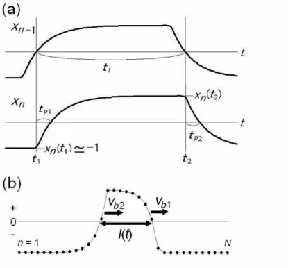
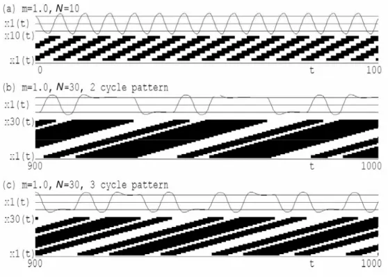
Figure 1(a) shows a spatiotemporal pattern of the unstable periodic solution of Eq. (1) with
N = 10, g = 10 and m = 0.2 under the initial condition Eq. (4) with l0 = N/2 = 5. A time series x1(t) of the state of the first neuron is shown in an upper panel. Black and white regions in a
lower panel correspond to the states of neurons of positive and negative values respectively. The network is divided into two blocks of equal numbers N/2 of neurons (black and white regions) and the signs of the states of neurons are the same in each block. The two boundaries of the blocks rotate in the network in the direction of the couplings with the same velocities. The states of neurons change their signs as the boundaries pass so that they oscillate. Since this periodic solution is unstable, the network starting from two blocks of unequal numbers of neurons converges to one of the steady states ±xp. Figure 1(b) shows a spatiotemporal pattern of the transient states of neurons under the initial condition Eq. (4) with l0 = 4 in the network
of N = 10. Then the velocities of the propagating boundaries slightly differ from each other. The number of neurons in a smaller block (l0 = 4) decreases and that in a larger block (l0 = 6)
increases. The boundaries then collide and the blocks merge so that the oscillation ceases. These behaviors are qualitatively the same as those of the network without inertia (m = 0, Eq. (2)). The duration of the transient oscillations increases exponentially with the number of neurons since difference between the velocities of the two boundaries decreases exponentially with the number of neurons in the blocks [18].
stable as the value of inertia increases. Figure 1(c) shows a spatiotemporal pattern of the transient states of neurons under the initial condition Eq. (4) with l0 = 2 in the network of N =
10 and large inertia m = 0.5. An initial pattern of unequal block lengths (l0 = 2 and N - l0 = 8)
approaches a symmetric pattern (l = 5) of the symmetric periodic solution, which is stabilized with inertia. In the following sections, we consider the duration and stability of the traveling waves and oscillations in the ring neural networks with inertia.
3. Kinematical description of traveling waves
In this section, we derive a kinematical model of the traveling boundaries of two blocks of neurons shown in Sect. 2. We replace f(x) with the following sign function, which corresponds to the limit of an output gain g → ∞.
sgn(x) = -1 (x ≤ 0)
= 1 (x > 0) (5)
The stable steady states of neurons are then given by xn = ± 1, yn = 0 (1 ≤ n ≤ N). Figure 2 shows a schematic diagram of changes in the states of the n-1st and nth neurons (a) and a spatial pattern of the states of neurons (b). Let t1 be the time at which the state xn-1 of the n-1st neuron changes from negative to positive, and t2 be the time at which xn-1 changes from positive to negative. That is, the boundaries b1 and b2 of the blocks of neurons pass the n-1st
neuron at t1 and t2 respectively. The input f(xn-1) to the nth neuron changes its sign at these times. We define the propagation time tp1 and tp2 of the boundaries at the nth neuron, i.e. time required for the propagation over one neuron, by
xn(t1 + tp1) = 0, xn(t2 + tp2) = 0 (6) The velocities vb1 and vb2 of the boundaries per neuron correspond to the inverses of the propagation times. They depend only on the states xn and yn of the nth neuron at t1 and t2
respectively.
Let vb2 (= 1/tp2) be considered. It is a function of xn(t2) and yn(t2). We can approximate xn(t2)
and yn(t2) by functions of the interval tl = t2 - t1 between the passages of the boundaries. That
is, we can approximate the states of the nth neuron at t1 by xn(t1) = -1 and yn(t1) = 0 since the states approach the steady states (-1, 0) exponentially and thus the effects of difference (xn(t1) - (-1) and yn(t1) - 0) on xn(t2) and yn(t2) at t2 are double exponentially small. The values of
(xn(t2), yn(t2)) is then given by the solution (x+(tl), y+(tl)) at t = tl (= t2 - t1) of the differential equation for a single neuron with the steady state (x+, y+) = (1, 0)
dx+/dt = y+, mdy+/dt = -y+ - x+ + 1, x+(0) = -1, y+(0) = 0 (7)
The values of the propagation time tp2 is calculated as the zero-crossing time of the state x- of
another single neuron with the steady state (x-, y-) = (-1, 0)
dx-/dt = y-, mdy-/dt = -y- - x- - 1, x-(0) = x+(tl), y-(0) = y+(tl), x-(tp2) = 0 (8) The propagation time tp2 and hence the velocity vb2 (= 1/tp2) of the boundary b2 are then expressed by a function of the interval tl (= t2 - t1) as
Let l be the number of neurons in the block of neurons of positive states (positive block) and N - l be that in the block of neurons of negative states (negative block) (Fig. 2(b)). We consider the number l of neurons to be the length of the block and a continuous variable. The interval tl = t2 - t1 is approximated with the length l of the positive block by
tl ≈ l/vb0 = tp0l (tl = t2 - t1, vb0 = 1/tp0)
dx-/dt = y-, mdy-/dt = -y- - x- - 1, x-(0) = 1, y-(0) = 0, x-(tp0) = 0 (10) where tp0 and vb0 correspond to the propagation time and velocity of the boundary respectively with the forward block of infinite length (l → ∞), in which the state of the nth neuron fully converges to the steady state (xn(t2), yn(t2)) = (1, 0) at t2. The velocity vb2 of the boundary b2 is then expressed by a function of the length l of the forward block by
substituting tl = l/vb0 in Eq. (10) into vb2(tl) in Eq. (9). The velocity vb1 of the other boundary is also expressed by the same function of the length N - l of the other block in the same way. Hence the propagation times and velocities of the two boundaries are expressed by common functions tp and vb of the lengths of their forward blocks respectively as
tp1 = tp((N - l)/vb0), tp2 = tp(l/vb0), vb1 = vb(N - l), vb2 = vb(l) (11) We then obtain kinematical description of changes in the block lengths (the numbers of neurons in the blocks) as
dl/dt = vb1 - vb2 = vb(N - l) - vb(l)
d(N - l)/dt = vb2 - vb1 = vb(l) - vb(N - l) (12) The steady states xn = -1 and 1 (yn = 0) of the network correspond to l(t) = 0 and N respectively. The symmetric periodic solution (Eq. (3)) corresponds to l(t) = N/2, which always exists irrespective of the form of vb(l). An initial block length is given by l(0) = l0 when the initial condition Eq. (4) is used for computer simulation of Eq. (1).
When inertia does not exist (m = 0), the velocity vb(l) of the boundary with the forward block length l is derived from Eq. (2) in the same way as above [18] and is given by
v'b(l) = v'b0 + k'exp(-c'l) (v'b0 = 1/log2, k' = v'b02 = 1/(log2)2, c' = 1/v'b0 = log2) (13) The velocity v'b(l) then monotonically decreases with l and the periodic solution (l(t) = N/2) is unstable since
dl/dt < 0 (l < N - l, i.e. 0 < l < N/2), dl/dt > 0 (l > N - l, i.e. N/2 < l < N) (14) Further, the stability of the periodic solution is tractable by letting l’ = l - N/2 in Eq. (12) dl’/dt = vb(N/2 - l’) - vb(N/2 + l’) = vl(l’; N, m, g)
vl(-l’; N, m, g) = -vl(l’; N, m, g) (15) where vl becomes an odd function of l' by definition. The periodic solution l(t) = N/2 corresponds to l’(t) = 0, and its stability depends on the sign of ∂vl(l’)/∂l’ at l’ = 0 as
∂vl(l’ = 0)/∂l’ > 0 (unstable)
< 0 (stable) (16)
When the value m of inertia increases, the velocity vb(l) can nonmonotonically changes with l since the approach of the states of neurons to the steady states becomes damped oscillatory (under damped). The periodic solution can then be stabilized through the pitchfork bifurcation at l’ = 0 since vl(l’) is an odd function [46]. A pair of unstable asymmetric periodic solutions is generated at the same time, which have two blocks of unequal lengths (the unequal numbers of neurons). Bifurcations and changes in the stability of the symmetric periodic solution due to inertia will be shown in Sect. 4.2.
4. Effects of inertia on the duration and stability of oscillations
Intuitively, the zero-crossing time tp(tl = l/vb0) in Eq. (11) is small (large) when the initial state x+(tl) is close to the origin (far from the origin) and y+(tl) is negative (positive). The velocity vb(l) (= 1/tp(l)) of the boundary at the nth neuron is then large (small) when the state
xn(t2) is close to the origin (far from the origin) and yn(t2) is negative (positive). When inertia is small (0 ≤ m ≤ 0.25), the characteristic equation of Eq. (7) has real negative roots (eigenvalues). The state x+(t) of the single neuron in Eq. (7) increases with t monotonically to
unity, and y+(t) decreases monotonically to zero (over damping (0 ≤ m < 0.25) and critical
damping (m = 0.25)). The velocity vb(l) of the boundary is then expected to decrease monotonically with the interval tl and hence with the length l of the forward block. The kinematical equation Eq. (12) of changes in the block length indicates that the symmetric periodic solution l(t) = N/2 is unstable owing to Eq. (14) as mentioned in Sect. 3. When inertia exceeds a critical value (m > 0.25), however, the characteristic roots of Eq. (7) become a complex conjugate pair so that the state x+ of the single neuron approaches
nonmonotonically to the steady state x+ = 1 (under damping (damped oscillation)). It is then
expected that the periodic solution is stabilized.
In this section, we show increases in the duration of transient oscillations due to inertia in an over damping mode in Sect. 4.1. The main result is given in Sect. 4.2, in which the stabilization of the periodic oscillations due to inertia in an under damping mode is shown. Further, bifurcations of periodic solutions of higher harmonics are shown with some examples in Sect. 4.3.
4.1 Increases in the duration of transient oscillations in over damping
Let 0 < m < 0.25 and then the state x+ of the single neuron in Eq. (7) is over damped. It is
expected that the symmetric periodic solution (l(t) = N/2) of Eq, (1) is unstable because of Eq. (14) since x+ increases monotonically to unity as mentioned above. When the initial condition
Eq. (4) with l0 ≠ N/2 is used, the traveling waves and oscillations are transient and the
network approaches one of the steady states (xn = ±xp, yn = 0 and l = 0, N). We here consider the duration of these transient oscillations.
Let two real negative characteristic roots of Eq. (7) be λ-- < λ+ < 0. Changes in the state
(x+(tl), y+(tl)) of the neuron around the steady state (1, 0) are dominated by the characteristic root λ+ of smaller absolute value. To obtain an explicit expression for the velocity vb(l) of the boundary with the forward block length l ((Eq. (11)), we approximate the solution (x+(tl),
x+(tb) ≈ -A+exp(-|λ+|tl) + 1, y+(tb) ≈ -λ+A+exp(-|λ+|tl)
A+ = [λ--(x+(0) + 1) + y+(0)]/(λ-+ - λ--) = 2λ--/(λ-+ - λ--) = [1 + (1 - 4m)1/2]/(1 - 4m)1/2
λ± = [-1 ± (1 - 4m)1/2]/(2m) (double signs in the same order) (17)
The solution x-(t) of Eq. (8) is also approximated by the term of λ+ as
x-(t) ≈ A+’exp(-|λ+|t) - 1 = [λ--(x-(0) + 1) + y-(0)]/(λ-+ - λ--)exp(-|λ+|t) - 1
≈ λ--(x-(0) +1)/(λ-+ - λ--)·exp(-|λ+|t) - 1 (18)
Using (x+(tl), y+(tl)) in Eq. (17) for (x-(0), y-(0)) in Eq. (18), we obtain the propagation time tp(tl) and velocity vb(l) of the boundary by solving x-(tp(tl)) = 0 in Eq. (18) as
tp(tl) ≈ {log(A+) + log[1 - exp(-|λ+|tl)]}/|λ+| ≈ tp0 - exp(-|λ+|tl)/|λ+|
vb(l) ≈ vb0[1 + exp(-|λ+|tl)/log(A+)] ≈ vb0[1 + exp(-|λ+|tp0l)/log(A+)]
tp0 = log(A+)/|λ+|, vb0 = 1/tp0 = |λ+|/log(A+) (tl = tp0l = l/vb0) (19) where tp0 and vb0 are the propagation time and velocity of the boundary respectively with infinite forward block length (tl, l → ∞), which correspond to those in Eq. (10). Substituting
vb(l) in Eq. (19) into Eq. (12), we obtain an explicit form of the kinematical equation of changes in the block length as
dl/dt = k{exp[-c(N - l)] - exp(-cl)}
k = vb0/log(A+) = |λ+|/[log(A+)]2, c = |λ+|tp0 = log(A+) (20)
When m = 0, the values of the parameters are: k = k' = 1/(log2)2 and c = c' = log2 in Eq. (13).
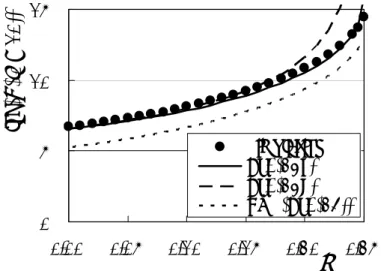
Figure 3 shows the velocity vb(l) of the boundary against the length l of the forward block when m = 0.1. Plotted are the velocity of the boundary in the periodic solutions obtained with computer simulation of Eq. (1) (solid circles), vb(l) in Eq. (11) derived through Eqs. (7 - 10) in Sect. 3 (a solid line), and vb(l) in Eq. (19) (a dashed line). The computer simulation of Eq. (1) was done using the Euler method with a time step 0.001 and N = 2l (2 ≤ l ≤ 15) under the initial condition Eq. (4) (l0 = l) so that the unstable periodic solutions were obtained. The
average velocities were calculated with 1000 rotations of the traveling boundaries in the network from t = 1000.0, at which the states of neurons fully converge to those of the periodic solutions. Values of vb(l) in Eq. (11) were given by vb2(tl) in Eq. (9) with tl = tp0l, in which tp2(tl) (= 1/vb2(tl)) were numerically calculated with Eqs. (7, 8), and tp0 was numerically calculated with Eq. (10). The velocity v'b(l) in Eq. (13) in the absence of inertia (m = 0) is also plotted with a dotted line. The velocity vb(l) for m = 0.1 decreases monotonically in the same manner as that in the absence of inertia. Both Eq. (19) and Eq. (9) agree with the simulation results of Eq. (1) except for small l (= 2).
Let an initial condition on Eq. (1) be Eq. (4) with 0 < l0 < N/2. The length l of the positive
block then decreases to zero owing to Eq. (14) and the network converges to the negative steady state (xn = -xp, yn = 0). The duration T of the transient oscillations of initial block length l0 is given by the zero-crossing time of Eq. (20) with
The duration T of the oscillations is then obtained in the same manner in the absence of inertia (m = 0) [18] as
T = 1/(ck)·exp(cN/2){arctanh[exp(c(l0 - N/2))] - arctanh[exp(-cN/2)]} (22)
Letting N → ∞ in Eq. (20) so that dl/dt = -kexp(-cl), a simple form of the duration is derived
T = [exp(cl0) - 1)]/(ck) (23a)
= tp0[exp(|λ+|tp0l0) - 1] (23b)
= log(A+)/|λ+|·[exp(log(A+)l0) - 1] (23c)
The duration thus increases exponentially as an initial block length l0 increases in the same
manner as that in the absence of inertia. (In the absence of inertia, it has been shown that Eq. (23) agrees with Eq. (22) when N = 40, and both agree with simulation results of Eq. (2) for l0
≥ 5 [18].) In the presence of inertia, the increasing rate of the duration with l0 depends on the
coefficient c (= |λ+|tp0 = log(A+)) in the exponential in Eq. (23). It can be shown that |λ+| in Eq.
(17) increases from unity to two when m increases from 0 to 0.25, while tp0 obtained with numerical calculation of Eq. (10) hardly changes. Further, the logarithm of A+ in Eq. (17)
monotonically increases from log2 at m = 0 as well, which diverges to infinity at m = 0.25. It is then expected that the logarithm of the duration of the transient oscillations increases about double from m = 0 to 0.25.
Figure 4 shows a semi-log plot of the duration T of the transient oscillations against m (0 ≤
m ≤ 0.25) for N = 30 and l0 = 10. Plotted are the results of computer simulation of Eq. (1)
under the initial condition Eq. (4) (solid circles), Eq. (23b) with |λ+| in Eq. (17) and tp0 numerically calculated with Eq. (10) (a solid line), and Eq. (23c) with |λ+| and A+ in Eq. (17)
(a dashed line). The value of the simulation result at m = 0.25 reaches more than double the value at m = 0 as expected, and Eq. (23b) agrees with the simulation results. Equation (23c) (a dashed line) agrees with the simulation results for m not close to 0.25 (0 ≤ m ≤ 0.2), while it tends to infinity as m → 0.25 with log(A+).
Further, the duration of the transient oscillations with initial block length l0 corresponds to
the relaxation time Tu of the unstable periodic solution in the network of N = 2l0. Numerical calculation can show that the periodic solution has the only positive characteristic exponent μ (the logarithm of the eigenvalue of the Poincare map), which means that it is one-dimensionally unstable. The relaxation time Tu is then evaluated with μ as
Tu = tp(l0/vb0)NNu = tp(l0/vb0)Nlog(1/z0)/μ ~ tp0N/μ (z0exp(μNu) = 1) (24) where Nu is the number of oscillations in the states of neurons (the number of rotations of boundaries) in the transient state, and z0 is an initial disturbance. The values of Tu (~ tp0N/μ) in the last line in Eq. (24) are also plotted in Fig. 4 (a dotted line). The values of μ were numerically calculated with the Poincare map of the periodic solutions of Eq. (1) with N = 20 (l0 = 10), and the values of tp0 were calculated with Eq. (10). The relaxation time Tu increases with m in the same manner as the simulation results. This agreement also supports the validity of the kinematical description of the traveling boundaries.
When inertia exceeds the critical value (m > 0.25), the state x+ of the single neuron in Eq.
(7) becomes under damped and its approach to the steady state becomes oscillatory. The characteristic equation of Eq. (7) has a complex conjugate pair of characteristic roots: λ± = [-1
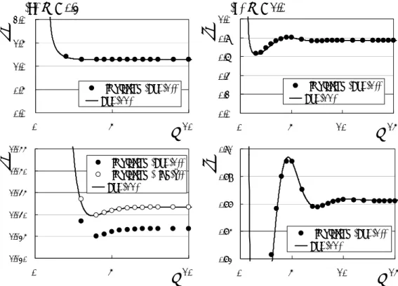
± i(4m - 1)1/2]/(2m). It is then expected that the approach of the velocity vb(l) of the boundary of the block to vb0 with l becomes oscillatory. Figure 5 shows the velocity vb(l) of the boundary against the length l of the forward block at m = 0.3 (a) and m = 1.0 (b). Lower panels are magnifications about vb0 (= vb(l → ∞)). Plotted are the averages of vb(l0) (l = l0) in 1000 rotations of the boundary in the symmetric periodic solution obtained with computer simulation of Eq. (1) with N = 2l0 under the initial condition Eq. (4) (solid circles) and vb(l) in Eq. (11) (solid lines). Here and in Figs. (6 - 8), values of vb(l) in Eq. (11) were numerically calculated with Eqs. (7 - 10) as mentioned in the explanation of Fig. 3. It can be seen that the velocity vb(l) once drops below vb0 and then increases to vb0 as l increases when m = 0.3 (a). More oscillations in vb(l) can be seen with further magnification. The simulation results of Eq. (1) in the lower panel are slightly smaller than vb(l) in Eq. (11), which is ascribed to difference in the output functions of neurons. The results of computer simulation using the sign function (Eq. (5)) for f(gx) in Eq. (1) are plotted with open circles, and vb(l) in Eq. (11) agree with them. The approach of vb(l) to vb0 in a form of damped oscillation is clear when m = 1.0 (b). It should be noted that, when the periodic solutions are stable, they can be obtained with computer simulation even though the number N of neurons is odd by using the initial condition Eq. (4) with xN/2(0) = 0. It should also be noted that vb(l) can be well fitted in a form of Aexp(-|Reλ±|l/vb0)cos(|Imλ±|l/vb0 + θ) + vb0 (l = vb0t) using the characteristic roots λ± of Eq. (7) for not so small l.
As mentioned in Sect. 3, the symmetric periodic solution (l(t) = N/2 in Eq. (12) and l’(t) = 0 in Eq. (15)) can be stabilized through the pitchfork bifurcation at l’ = 0 when vb(l) and vl(l’;
N, m, g) become nonmonotonic as m increases [46]. At the same time a pair of unstable
asymmetric periodic solutions is generated, which are traveling waves with two blocks of unequal lengths. The bifurcation occurs when the length at the minimal point in the graph of
vb(l) decreases to N/2 as m increases so that dvb(l = N/2)/dl = 0 and ∂vl(l’ = 0)/∂l’ = 0. The period To of the damped oscillation in Eq. (7) is 2π/|Imλ±| = 4mπ/(4m - 1)1/2, which quickly
decreases as m increases over 0.25. The length at the minimal of vb(l) decreases along with the spatial period To/tp0 of the damped oscillation. Hence the length at the mininal also decreases quickly with m since the propagation time tp0 changes only slightly with m as mentioned in Sect. 4.1. When the slope of the graph of vb(l) becomes positive at l = N/2 (dvb(l = N/2)/dl > 0) and hence ∂vl(l’ = 0)/∂l’ < 0, the symmetric periodic solution is stabilized. Figure 6 shows vl(l’; N, m, g) in Eq. (15) obtained with numerically calculated vb(l) in Eq. (11). The number of neurons is N = 10, and m = 0.1 (a solid line), m = 0.3 (a dashed line) and
m = 1.0 (a dotted line). The graph for m = 0.1 increases monotonically with m and the slope at l’ = 0 is positive (∂vl(l’ = 0)/∂l’ > 0). Hence the symmetric periodic solution (l(t) = N/2 = 5) is still unstable. However, there are two zero-crossing points on both sides of l’ = 0 in the graph for m = 0.3 with the negative slope at l’ = 0 (∂vl(l’ = 0)/∂l’ < 0). The symmetric periodic solution is then stabilized when m = 0.3 and a pair of unstable asymmetric periodic solutions with unequal block lengths (lu and N - lu, lu ≈ 3.1) is generated. Further, the pitchfork bifurcation occurs again as m increases, and there are five zero-crossing points in the graph of
m = 1.0 so that the symmetric periodic solution becomes unstable again (∂vl(l’ = 0)/∂l’ > 0). A pair of stable asymmetric periodic solutions of block lengths (ls and N - ls, ls ≈ 3.7) is also generated.
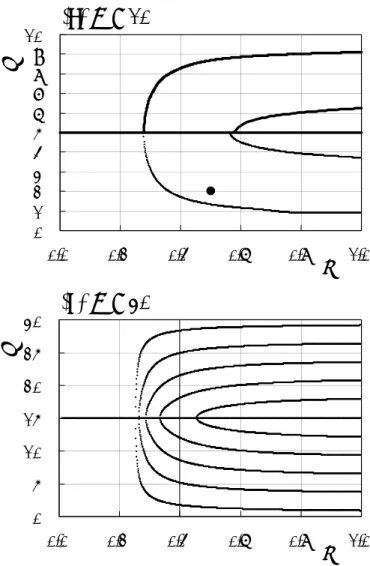
Figure 7(a) shows a bifurcation diagram of the periodic solutions l(t) = l with m in the network of N = 10. Plotted are the sums /2 /2
1 L x L n n −
∑
=of the states of neurons in the periodic solutions of Eq. (1) calculated numerically (solid lines) in an upper half region (l ≥
also are the lengths l at which ∂vl(l’)/∂l’ = 0 (l’ = l - N/2) in Eq. (15) (small dots) in a lower half region (l < 5). They are plotted separately for visibility since the bifurcations are always symmetric with respect to l = N/2. Both bifurcation diagrams agree with each other except for
m ≈ 0.57 (the second bifurcation point). The symmetric periodic solution (l(t) = N/2) becomes
stable and a pair of unstable branches bifurcates at m ≈ 0.27 through the subcritical pitchfork bifurcation. The two bifurcated branches correspond to a pair of asymmetric periodic solutions with blocks of unequal lengths, in which the length of a positive block is smaller (l < N/2) or larger (l > N/2). The steady states (l(t) = 0, N) are still stable, and the unstable asymmetric periodic solutions are the separatrices of the steady states and the symmetric periodic solution. It can be seen that the initial length l0 = 2 (N = 10) at m = 0.5 in Fig. 1(c),
the point of which is denoted with a solid circle, lies in the basin of the symmetric periodic solution so that l approaches N/2. Further, the second pitchfork bifurcation occurs at m ≈ 0.57 so that the symmetric periodic solution becomes unstable again and a pair of stable asymmetric periodic solutions is generated. Small difference at m ≈ 0.57 between the graphs obtained with Eq. (15) in the upper half region and Eq. (1) in the lower half region is ascribed to the fact that changes in the characteristic roots λ± of Eq. (7) and hence vb(l) with m become small when m is large, i.e. vb(l)/dm → 0 as m → ∞. Difference due to approximation with the kinematical model is then manifested. In fact, it can be shown that they slightly differ in the flat regions of the bifurcated branches also.
The cascade of bifurcations occurs when the number N of neurons is large. Figure 7(b) shows a bifurcation diagram of the periodic solutions in the network of N = 30, in which the bifurcations of the symmetric periodic solution occur five times as m increases. Plotted are only the lengths l at which ∂vl(l’)/∂l’ = 0 (l’ = l - N/2) in Eq. (15) (small dots). It is difficult to trace the bifurcations of the periodic solutions of Eq. (1) numerically for such large N since the absolute values of the characteristic exponents μ of the periodic solutions decrease to zero exponentially with N, so that the convergence of calculation is too slow. A total of thirteen solutions then coexist when the value m of inertia exceeds the fifth bifurcation point (m > 0.46), in which seven are stable, namely the symmetric periodic solution, two pairs of asymmetric periodic solutions and a pair of steady states. The numbers of bifurcations and generated branches depend on the spatial period To/tp0 of the damped oscillation in Eq. (7) and vb(l). The period To (= 4mπ/(4m - 1)1/2) of the damped oscillation takes the minimum value 2π at m = 0.5 and then increases in proportion about to m1/2, while the propagation time
tp0 also increases with m. Numerical calculation can show that the spatial period T/tp0 takes the minimum value (≈ 5.55) at m ≈ 2.0 and then increases only slightly with m, e.g. To/tp0 ≈ 5.7 at m = 10.0. No more branches thus bifurcate even though m increases over two.
The bifurcations of the periodic solution also occur as the number N of neurons increases in vl(l’; N, m, g) in Eq. (15). Figure 8 shows a bifurcation diagram of the symmetric periodic solution l(t) = N/2 in the (m, N) plane. Small dots denote the bifurcation points at which ∂vl(l’)/∂l’ = 0 at l’ = 0 (l’ = l - N/2) in Eq. (15), which were calculated by changing N for each
m and obtained formally even for non-integer N. Solid and open circles on the lines of N = 2i
(2 ≤ i ≤ 10) denote the bifurcation points of the symmetric periodic solution of Eq. (1) calculated numerically using the Poincare map, at which the characteristic exponent μ of it crosses zero from positive to negative (open circles) and from negative to positive (solid circles) as m increases so that the stability changes. The symmetric period solution is unstable and stable in the regions denoted with “+” and “-“, respectively. The bifurcation points of Eq. (15) agree with those of the periodic solution of Eq. (1) for N ≤ 20. The characteristic exponent of the periodic solution for larger N is difficult to calculate numerically as mentioned above. Finally, it should be noted that it can be shown that the bifurcations of the periodic solution also occur with g in vl(l’; N, m, g) in Eq. (15), but they can not be treated with the kinematical model since the sign function (Eq. (5)) is used in its derivation.
4.3 Bifurcations of periodic solutions of higher harmonics
We restricted ourselves to the bifurcations of the periodic solution with two blocks of neurons in Sect. 4.2. It is known, however, that there are not more than (N - 2)/4 unstable periodic solutions in the network with m = 0 in Eq. (2) when an output gain g is large, which are generated through the successive Hopf bifurcations at the origin [15]. These multiple periodic solutions are traveling waves of higher harmonics, in which the numbers of blocks are 2kb (2 ≤ kb ≤ (N - 2)/4) and the numbers of neurons in the blocks are nb = N/(2kb) (N/4 ≥
nb > 2). These periodic solutions have 2kb - 1 positive real characteristic exponents and are (2kb - 1)-dimensionally unstable. Numerical calculation can show that they also exist in the networks with inertia. They can then be stabilized as inertia increases through the pitchfork bifurcation in the same manner as that shown in Sect. 4.2.
Figure 9(a) shows a spatiotemporal pattern of the states of neurons approaching a stable periodic solution with four blocks of equal lengths in Eq. (1) with N = 10 and m = 1.0, which was obtained with computer simulation under the initial condition that (x1(0), …, x10(0)) = (1,
1, -1, -1, -1, 1, 1, -1, -1, -1) and yn(0) = 0 (1 ≤ n ≤ 10). As the number N of neurons increases, more periodic solutions of higher harmonics coexist and they are also stabilized. Further, stable asymmetric periodic solutions of higher harmonics are generated from them through the pitchfork bifurcations of the second, fourth times and so on. The networks of large numbers of neurons show stable oscillations of various patterns. Figure 9(b) and (c) show spatiotemporal patterns of two and three cycle asymmetric stable periodic oscillations respectively obtained with computer simulation of Eq. (1) under random initial conditions in the network of N = 30 and m = 1.0. Intuitively, periodic solutions with even numbers 2kb (≤ (N - 2)/4) of blocks of lengths li (1 ≤ i ≤ 2kb) are stable when
v l v v l l l i k l L kb i i b i b kb i b = = > ≤ ≤
∑
= = 2 1 2 , d ( )/d 0 (1 2 ), ) ( (25)Since regions in which the block lengths are stable (dvb(l)/dl > 0) exist in every cycle of the damped oscillation in vb(l) (0 ≤ l ≤ N), the number nl of the stable lengths increases in proportion to the number N of neurons. The number of stable periodic solutions thus increases exponentially with the number of neurons since it increases in a form of the nlth power of 2.
Further, numerical calculation can show that pairs of characteristic exponents of the periodic solutions of higher harmonics of Eq. (1) become complex conjugates in the presence of inertia. The Neimark-Sacker bifurcations then occur and unstable aperiodic solutions are generated as m increases before the higher harmonics are stabilized through the pitchfork bifurcations. The kinematical description of changes in the block length can be extended to the traveling wave of higher harmonics with 2kb blocks, which is a (2kb - 1)-dimensional system of first-order differential equations for 2kb - 1 block lengths. In this kinematical model of the lengths of the traveling blocks of neurons, the Hopf bifurcations occur and unstable periodic solutions are generated. It is then expected that the lengths of the blocks oscillate periodically in the aperiodic solutions, though they can not be obtained in computer simulation of Eq. (1) owing to their instability.
5. Circuit experiment
Figure 10 shows an analog circuit of the ring neural network with inertia (Eq. (1)). Voltages Vn at capacitors C and nonlinear amplifiers of gain g correspond to the states xn and
output functions f(x) of neurons respectively. A total of N elements are connected in series with resistances R and inductors L and the output f(xN) of the Nth element is fed back to the first element. The sigmoidal function f(x) is replaced with the step function of the inverter TC4049: Vout = 0V for Vin > 2.5V, Vout = 5V for Vin < 2.5V with the supply voltage 5V. Note that this network of inhibitory (negative) couplings is equivalent to that of excitatory (positive) couplings under changes in the signs of the states of even neurons when the total number N of neurons is even. The circuit equation is given by
LCdVn2/dt2 + CRdVn/dt + V + Vout(Vn-1) = 0 (V0 = VN, 1 ≤ n ≤ N) (26) Inertia takes a form m = L/(R2C) when time is rescaled with a time constant RC (t ← t/(RC)).
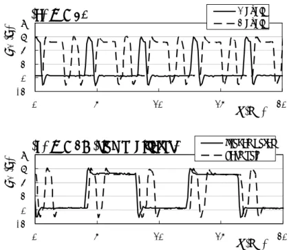
The values of parameters were: L = 100mH, R = 1kΩ, C = 0.1μF, and DC resistance of the inductor is 65Ω max. The value of inertia was then about unity (m ≈ 1.0) and the time constant was 0.1ms. A circuit with thirty elements (N = 30) was made. Stable oscillations were easily obtained by adding periodic signals of appropriate frequency to one element or even with switching noise. Figure 11(a) shows observed time series of the voltage V1 at the
first element, in which asymmetric one cycle pattern (a solid line) and two cycle patterns (a dashed line) are plotted. The periods of the oscillations are about 4.2ms and the velocity vb0 of the traveling boundary per neuron is 30/(4.2/0.1) ≈ 0.71 per time constant. This agrees about with vb0 (≈ 0.77) in Fig. 5(b).
The reason for using not buffers but inverters is that circuits with buffers (TC4050) had not shown expected stable oscillations when the number of elements increases (e.g. N > 15) in a preliminary experiment. It is due probably to asymmetry in high, threshold and low voltage values of the buffer IC, which makes the output functions of neurons asymmetric. In fact, it has been shown that small offset voltages in operational amplifiers in analog circuits of the ring neural networks without inertia degrade exponential increases in the duration of transient oscillations [18]. Average asymmetry in the output functions of neurons due to variations in the elements causes constant velocities in the kinematical equation of the traveling boundaries of the blocks [47]. These constant velocities can overtake changes in the velocities due to inertia so that the velocities of two boundaries are never the same and the networks remain globally bistable. By using inverters the asymmetry is about canceled out on average and the constant velocities are reduced.
It is known that the occurrence of multiple modes of oscillations happens in ring oscillators, which consist of odd numbers of inverters and show stable oscillations [13]. In the ring neural network of ring oscillator type, in which couplings are negative and the number of neurons is odd, there is one inconsistency in the states of neurons, i.e. the same signs of the states of two successive neurons as (+, -, +, +, -, +, -). The inconsistency rotates in the direction of couplings so that the states of neurons change their signs when the inconsistency passes them. They then oscillate once when the inconsistency rotates twice in the network, which is like the Möbius band. More than one inconsistencies of odd numbers can exist and rotate in the network, which correspond to oscillations of higher harmonics. The kinematics of the traveling waves in the ring neural networks without inertia (Eq. (2)) shows that these higher harmonics are unstable [18]. However, they may be stabilized owing to effective/equivalent series inductance in actual circuits of ring oscillators, in which usually inverters are directly connected without any passive elements. Figure 11(b) shows time series of the voltage V1
observed in the analog circuit with an odd number of elements (N = 29). The circuit shows stable oscillations of ring oscillator type. In addition to an oscillation of fundamental frequency (a solid line), in which one inconsistency is rotating in the network, an asymmetric oscillation of higher harmonics is observed (a dashed line), in which three inconsistencies are stably rotating.
6. Conclusion and future work
It was shown that inertia (inductive couplings) changes properties of bistable ring neural networks qualitatively. It is known that the networks without inertia show transient oscillations, in which neurons divided in even blocks with the signs of their states, and the boundaries of the blocks rotate in the networks. These traveling waves are unstable and eventually the boundaries collide so that the oscillations cease. Difference between the velocities of the boundaries decreases exponentially with the numbers of neurons in the blocks, however, so that the transient oscillations last exponentially long. The kinematical model of the traveling boundaries between two blocks of neurons was generalized in the presence of inertia. The recovery process of each neuron becomes from over damped (monotonic) to under damped (oscillatory) as inertia increases. In an over damping mode, difference between the velocities of two boundaries becomes small as inertia increases up to critical damping since the convergence of the state of a single neuron to its steady state becomes fast. The convergence of the network to one of the steady states then becomes slow and the increasing rate of the logarithm of the duration of the transient oscillations becomes more than twice as large as that without inertia. Thus inertia enforces exponential increases in transient time with system size. In an under damping mode, the velocities of the boundaries change nonmonotonically with the number of neurons in the forward blocks. The symmetric periodic solution, which is the traveling wave with two blocks of the same numbers of neurons, is then stabilized through the pitchfork bifurcation as inertia increases. A succession of the pitchfork bifurcations occur as inertia increases further, so that the symmetric and asymmetric periodic solutions and the steady states coexist in the networks with large inertia. Further, the bifurcations and stabilization of the periodic solutions of higher harmonics also occur and oscillations of various patterns coexist in the networks of large numbers of neurons.
As mentioned in Sect. 4.3, not only periodic oscillations but also aperiodic oscillations can be generated through the Neimark-Sacker bifurcations as inertia increases. It is probable that the networks show chaotic behaviors in the presence of external forces or interaction between networks. The structure of global bifurcations and basins of attractors in the high-dimensional spaces of the networks are of interest. (The dimension is equal to twice the number of neurons.) Kinematical description of the traveling waves in the networks might be useful for studies on them. Further, it is known that spatial variations and spatiotemporal noise in the ring neural networks without inertia degrade exponential increases in the duration of the oscillations as mentioned in Sect. 5. In fact, stable oscillations had been hard to observe in circuits with positive couplings owing to asymmetry in a buffer IC. Effects of variations and noise on the bifurcations of periodic solutions and the stability of oscillations in the networks with inertia are also of interest.
References
[1] J. J. Collins and I. Stewart, A group-theoretic approach to rings of coupled biological oscillators, Biol. Cybern. 71 (1994) pp. 95-103.
[2] E. Marder and R. L. Calabrese, Principles of rhythmic motor pattern production. Physiol. Rev. 76 (1996) pp. 687–717.
[3] S. Amari, Mathematics of Neural Networks (in Japanese), Sangyo-Tosho, Tokyo (1978). [4] M. H. Hirsh, Convergent activation dynamics in continuous time networks, Neural Networks 2 (1989) pp. 331-340.
exploration of the labeling hypothesis, Int. J. Neural Systems 1 (1989) pp. 103-124.
[6] T. Gedeon, Cyclic Feedback Systems, Memoirs of the American Mathematical Society, American Mathematical Society (1998).
[7] F. Pasemann, Characterization of periodic attractors in neural ring networks, Neural Networks 8 (1995) pp. 421-429.
[8] S. Guo and L. Huang, Pattern formation and continuation in a trineuron ring with delays, Acta Mathematica Sinica 23 (2007) pp. 799-818.
[9] X. Xu, Complicated dynamics of a ring neural network with time delays, J. Phys. A 41 (2008) 035102 (23pp).
[10] K. L. Babcock and R. M. Westervelt, Dynamics of simple electronic neural networks, Physica D 28 (1987) pp. 305-316.
[11] P. Baldi and A. F. Atiya, How delays affect neural dynamics and learning, IEEE Trans. Neural Networks 5 (1994) pp. 612-621.
[12] K. Pakdaman, C. P. Malta, C. Grotta-Ragazzo, O. Arino and J.-F. Vibert, Transient oscillations in continuous-time excitatory ring neural networks with delay, Phys. Rev. E 55 (1997) pp. 3234-3248.
[13] J. G. Webster (Ed.), Wiley Encyclopedia of Electrical and Electronics Engineering 23, John Wiley, 1999, pp. 79-80.
[14] T. Ishii and H. Kitajima, Oscillation in cyclic coupled neurons, Proc. 2006 RISP Int. Workshop on Nonlinear Circuits and Signal Processing (NCSP2006), 2006, pp. 97-100. [15] H. Kitajima, T. Ishii and T. Hattori, Oscillation mechanism in cyclic coupled neurons, Proc. 2006 Int. Symp. on Nonlinear Theory and its Applications (NOLTA 2006), 2006, pp. 623-626.
[16] H. Kitajima and Y. Horikawa, Oscillation in cyclic coupled systems, Proc. 2007 Int. Symp. on Nonlinear Theory and its Applications (NOLTA 2007), 2007, pp. 453-456.
[17] Y. Horikawa and H. Kitajima, Experiments on transient oscillations in a circuit of diffusively coupled inverting amplifiers, Proc. 19th Int. Conf. on Noise and Fluctuations (ICNF2007), in M. Tacano, et al. (Eds.), Noise and Fluctuations: 19th International Conference on Noise and Fluctuations; ICNF 2007 (Conference Proceedings Series 922), AIP, 2007, pp. 569-572.
[18] Y. Horikawa and H. Kitajima, Duration of transient oscillations in ring networks of unidirectionally coupled neurons, Physica D 238 (2009) pp. 216-225.
[19] H. Kitajima and Y. Horikawa, Mechanism of long transient oscillations in cyclic coupled systems, Chaos, Solitons and Fractals (2009) pp. 1854-1859.
[20] K. Kawasaki and T. Ohta, Kink dynamics in one-dimensional nonlinear systems, Physica 116A (1982) pp. 573-593.
[21] J. Carr and R. L. Pego, Metastable patterns in solutions of u = εu - f(u), Commun. Pure Appl. Math. 42 (1989) pp. 523-576.
[22] S. Ei and T. Ohta, Equation of motion for interacting pulses, Phys. Rev. E 50 (1994) pp. 4672 - 4678.
[23] Y. Horikawa, Duration of transient fronts in a bistable reaction-diffusion equation in a one-dimensional bounded domain, Phy. Rev. E 78 (2008) pp. 066108/1-10.
[24] M. J. Ward, Metastable bubble solutions for the Allen-Cahn equation with mass conservation, SIAM J. Appl. Math. 56 (1996) pp. 1247-1279.
[25] M. J. Ward, Dynamic metastability and singular perturbations, in M. C. Delfour (Ed.), Boundaries, Interfaces, and Transitions (CRM Proceedings and Lecture Notes 13), AMS, 1998, pp. 237-263.
[26] K. Kaneko, Supertransients, spatiotemporal intermittency and stability of fully developed spatiotemporal chaos, Phys. Lett. A 149 (1990) pp. 105-112.
[27] A. Wacker, S. Bose and E. Schöll, Transient spatio-temporal chaos in a reaction-diffusion model, Europhysics Letters 31 (1995) pp. 257-262.
[28] R. Zillmera, R. Livib, A. Politic and A. Torcini, Desynchronized stable states in diluted neural networks, Neurocomputing 70 (2007) pp. 1960-1965.
[29] U. Bastolla and G. Parisi, Relaxation, closing probabilities and transition from oscillatory to chaotic attractors in asymmetric neural networks, J. Phys. A 31 (1998) pp. 4583-4602. [30] J. Šíma and P. Orponen, Exponential transients in continuous-time Liapunov systems, Theoretical Computer Science 306 (2003) pp. 353-372.
[31] K. L. Babcock and R. M. Westervelt, Stability and dynamics of simple electronic neural networks with added inertia, Physica D 23 (1986) pp. 464-469.
[32] D. W. Wheeler and W. C. Schieve, Stability and chaos in an inertial two-neuron system, Physica D 105 (1997) pp. 267-284.
[33] J. Hertz, A. Krogh and R. G. Palmer, Introduction to the Theory of Neural Computation, Addison-Wesley (1991).
[34] K. S. Cole, Membranes, Ions and Impulses: A Chapter of Classical Biophysics, University of California Press (1968).
[35] R. FitzHugh, Impulse and physiological states in theoretical models of nerve membrane, Biophys. J. 1 (1961) pp. 445-466.
[36] J. Nagumo, S. Arimoto and S. Yoshizawa, An active pulse transmission line simulating nerve axon, Proc. IRE 50 (1962) pp. 2061-2070.
[37] H. Tanaka, A. J. Lichtenberg and S. Oishi, Self-synchronization of coupled oscillators with hysteretic responses, Physica D 100 (1997) pp. 279-300.
[38] H Hong, et al., Noise effects on synchronization in systems of coupled oscillators, J. Phys. A 32 (1999) pp. L9-L15.
[39] J. A. Acebrón, L. L. Bonilla and R. Spigler, Synchronization in populations of globally coupled oscillators with inertial effects, Phys. Rev. E 62 (2000) pp. 3437-3454.
[40] G.. B. Ermentrout, An adaptive model for synchrony in the firefly Pteroptyx malaccae, J. Math. Biol. 29 (1991) pp. 571–585.
[41] K. Dolana, M. Majtanika and P. A. Tass, Phase resetting and transient desynchronization in networks of globally coupled phase oscillators with inertia, Physica D 211 (2005) pp. 128-138.
[42] H. Haken, Brain Dynamics, Springer-Verlag, Berlin (2002).
[43] T. Endo and S. Mori, Mode analysis of a multimode ladder oscillator Circuits and Systems, IEEE Trans. Circuits & Syst. 23 (1976) pp. 100-113.
[44] S. Datardina and D. Linkens, Multimode oscillations in mutually coupled van der Pol type oscillators with fifth-power nonlinear characteristics, IEEE Trans. Circuits & Syst. 25 (1978) pp. 308-315.
[45] M. Yamauchi, Y. Nishio and A. Ushida, Phase-waves in a ladder of oscillators, IEICE Trans. E86 (2003) pp. 891-899.
[46] S. Wiggins, Introduction to Applied Nonlinear Dynamical Systems and Chaos, Springer (1990).
[47] Y. Horikawa and H. Kitajima, Effects of noise and variations on the duration of transient oscillations in unidirectionally coupled bistable ring networks, Phys. Rev. E 80 (2009) pp. 021934/1-15.
Figure captions
Fig. 1. Spatiotemporal patterns of the states of neurons in Eq. (1) with N = 10 and g = 10. Upper panels: time series x1(t) of the state of the first neuron. Lower panels: the states of
neurons (positive: black, negative: white). Periodic oscillation with m = 0.2 and l0 = N/2 = 5
(a), transient oscillation with m = 0.2 and l0 = 4 (b) and persistent oscillation with m = 0.5 and l0 = 2 (c).
Fig. 2. Schematic diagram of changes in the states of the n-1st and nth neurons (a) and a spatial pattern of the states of neurons (b).
Fig. 3. Velocity vb(l) of the boundary vs the length l of the forward block (m = 0.1). Computer simulation of Eq. (1) (solid circles), Eq. (11) (a solid line), and Eq. (19) (a dashed line). Eq. (13) for m = 0 is also plotted with a dotted line.
Fig. 4. Semi-log plot of the duration T of transient oscillations vs m (0 ≤ m ≤ 0.25) for N = 20 and l0 = 10. Computer simulation of Eq. (1) under Eq. (4) (solid circles), Eq. (23b) with
|λ+| in Eq. (17) and tp0 in Eq. (10) (a solid line), Eq. (23c) with |λ+| and A+ in Eq. (17) (a dashed line), and the relaxation time Tu in Eq. (24) of the periodic solution of Eq. (1) with N = 20 (l0 = 10) (a dotted line).
Fig. 5. Velocity vb(l) of the boundary vs the length l of the forward block with m = 0.3 (a) and m = 1.0 (b). Averages of vb(l0) in 1000 rotations in computer simulation of Eq. (1) with N
= 2l0 (solid circles) and vb(l) in Eq. (11) (solid lines).
Fig. 6. vl(l’; N, m, g) in Eq. (15) with N = 10 for m = 0.1 (a solid line), m = 0.3 (a dashed line) and m = 1.0 (a dotted line).
Fig. 7. Bifurcation diagram of the periodic solution l with m in the network of N = 10 (a) and N = 30 (b). Sums /2 /2 1 L x L n n −
∑
=in the periodic solutions of Eq. (1) (solid lines) in an upper half region (l ≥ N/2 = 5) in (a) and lengths l at which ∂vl(l’)/∂l’ = 0 (l’ = l - N/2) in Eq. (15) (small dots) in a lower half region (l < 5) in (a) and in (b).
Fig. 8. Bifurcation diagram of the symmetric periodic solution l(t) = N/2 in the (m, N) plane. Bifurcation points at which ∂vl(l’)/∂l’ = 0 in Eq. (15) (small dots) and the bifurcation points of the periodic solutions of Eq. (1) (open and solid circles).
Fig. 9. Spatiotemporal patterns of the periodic solutions of Eq. (1) with m = 1.0 and N = 10 (a), N = 30 (b) (c).
Fig. 10. Analog circuit of the ring neural network with inertia.
Fig. 11. Time series of the voltage V1 in the analog circuit with N = 30 (a) and N = 29 (ring
Figures
Fig. 1. Spatiotemporal patterns of the states of neurons in Eq. (1) with N = 10 and g = 10. Upper panels: time series x1(t) of the state of the first neuron. Lower panels: the states of
neurons (positive: black, negative: white). Periodic oscillation with m = 0.2 and l0 = N/2 = 5
(a), transient oscillation with m = 0.2 and l0 = 4 (b) and persistent oscillation with m = 0.5 and l0 = 2 (c).
Fig. 2. Schematic diagram of changes in the states of the n-1st and nth neurons (a) and a spatial pattern of the states of neurons (b).
Fig. 3. Velocity vb(l) of the boundary vs the length l of the forward block (m = 0.1). Computer simulation of Eq. (1) (solid circles), Eq. (11) (a solid line), and Eq. (19) (a dashed line). Eq. (13) for m = 0 is also plotted with a dotted line.
Fig. 4. Semi-log plot of the duration T of transient oscillations vs m (0 ≤ m ≤ 0.25) for N = 20 and l0 = 10. Computer simulation of Eq. (1) under Eq. (4) (solid circles), Eq. (23b) with
|λ+| in Eq. (17) and tp0 in Eq. (10) (a solid line), Eq. (23c) with |λ+| and A+ in Eq. (17) (a
dashed line), and the relaxation time Tu in Eq. (24) of the periodic solution of Eq. (1) with N = 20 (l0 = 10) (a dotted line). 0 5 10 15 0.00 0.05 0.10 0.15 0.20 0.25
m
lo
g(
T
(
l
0=
10)
)
simulation Eq. (23b) Eq. (23c) Tμ (Eq. (24)) 0.0 0.5 1.0 1.5 2.0 2.5 0 5 10 15l
v
b simulation (Eq. (1)) Eq. (11) Eq. (19) m = 0 (Eq. (13))Fig. 5. Velocity vb(l) of the boundary vs the length l of the forward block with m = 0.3 (a) and m = 1.0 (b). Averages of vb(l0) in 1000 rotations in computer simulation of Eq. (1) with N
= 2l0 (solid circles) and vb(l) in Eq. (11) (solid lines).
Fig. 6. vl(l’; N, m, g) in Eq. (15) with N = 10 for m = 0.1 (a solid line), m = 0.3 (a dashed line) and m = 1.0 (a dotted line).
-0.10 -0.05 0.00 0.05 0.10 -5 -4 -3 -2 -1 0 1 2 3 4 5
l
'
v
l m = 0.1 m = 0.3 m = 1.0 (a) m = 0.3 0.0 0.5 1.0 1.5 2.0 0 5 10l
v
b simulation (Eq. (1)) Eq. (11) 1.130 1.135 1.140 1.145 1.150 1.155 0 5 10l
v
b simulation (Eq. (1)) simulation (sign(x)) Eq. (11) (b) m = 1.0 0.0 0.2 0.4 0.6 0.8 1.0 0 5 10 15l
v
b simulation (Eq. (1)) Eq. (11) 0.73 0.75 0.77 0.79 0.81 0 5 10 15l
v
b simulation (Eq. (1)) Eq. (11)Fig. 7. Bifurcation diagram of the periodic solution l with m in the network of N = 10 (a) and N = 30 (b). Sums /2 /2 1 L x L n n −
∑
=in the periodic solutions of Eq. (1) (solid lines) in an upper half region (l ≥ N/2 = 5) in (a) and lengths l at which ∂vl(l’)/∂l’ = 0 (l’ = l - N/2) in Eq. (15) (small dots) in a lower half region (l < 5) in (a) and in (b).
(a)
N
= 10
0 1 2 3 4 5 6 7 8 9 10 0.0 0.2 0.4 0.6 0.8 1.0 ml
(b)
N
= 30
0 5 10 15 20 25 30 0.0 0.2 0.4 0.6 0.8 1.0 ml
Fig. 8. Bifurcation diagram of the symmetric periodic solution l(t) = N/2 in the (m, N) plane. Bifurcation points at which ∂vl(l’)/∂l’ = 0 in Eq. (15) (small dots) and the bifurcation points of the periodic solutions of Eq. (1) (open and solid circles).
Fig. 9. Spatiotemporal patterns of the periodic solutions of Eq. (1) with m = 1.0 and N = 10 (a), N = 30 (b) (c). 0 10 20 30 40 0.0 0.2 0.4 0.6 0.8 1.0
m
N
Fig. 10. Analog circuit of the ring neural network with inertia.
Fig. 11. Time series of the voltage V1 in the analog circuit with N = 30 (a) and N = 29 (ring
oscillator type) (b). (b) N = 29 (ring oscillator) -2 0 2 4 6 8 0 5 10 15 20 t (ms) V1 ( V ) fundamental harmonics (a) N = 30 -2 0 2 4 6 8 0 5 10 15 20 t (ms) V1 (V ) 1 cycle 2 cycle