Panel Data Research Center at Keio University
DISCUSSION PAPER SERIES
DP2013-001 July, 2013
Well-being effects of a major negative externality: The case of Fukushima
Katrin Rehdanza,b Heinz Welschc
Daiju Naritaa Toshihiro Okubod
【Abstract】
Following a major earthquake off the Pacific coast of Japan, a tsunami disabled the power supply and cooling of three reactors in Fukushima, causing a major nuclear accident on 11 March 2011. Based on a quasi-experimental difference-in-differences approach we use panel data for 5,979 individuals interviewed in Japan before and after the accident to analyze the effect of the accident on people’s subjective well-being. Our main hypotheses are that this effect declines with distance to the place of the event but also with distance to other nuclear power plants. To test these hypotheses, we use Geographical Information Systems to merge the well-being data with information on respondents’ distance to the Fukushima nuclear plant and on their proximity to nuclear power stations in general. Our empirical results suggest the existence of significant well-being effects of the combined event of the earthquake, tsunami and nuclear accident that are proportional to proximity to the Fukushima site being equivalent to up to 72 percent of annual household income. We find no evidence for increased nation-wide worry about the presence of nuclear power plants near people’s place of residence.
a Kiel Institute for the World Economy, Kiel, Germany b Kiel University, Department of Economics, Kiel, Germany
c University of Oldenburg, Department of Economics, Oldenburg, Germany d Keio University, Faculty of Economics, Tokyo, Japan
Panel Data Research Center at Keio University Keio University
1
Well-being effects of a major negative externality: The case of Fukushima
Katrin Rehdanza,b,*, Heinz Welschc , Daiju Naritaa and Toshihiro Okubod
a
Kiel Institute for the World Economy, Kiel, Germany
b
Kiel University, Department of Economics, Kiel, Germany
c
University of Oldenburg, Department of Economics, Oldenburg, Germany
d
Keio University, Faculty of Economics, Tokyo, Japan
Abstract
Following a major earthquake off the Pacific coast of Japan, a tsunami disabled the power supply and cooling of three reactors in Fukushima, causing a major nuclear accident on 11 March 2011. Based on a quasi-experimental difference-in-differences approach we use panel data for 5,979 individuals interviewed in Japan before and after the accident to analyze the effect of the accident on people’s subjective well-being. Our main hypotheses are that this effect declines with distance to the place of the event but also with distance to other nuclear power plants. To test these hypotheses, we use Geographical Information Systems to merge the well-being data with information on respondents’ distance to the Fukushima nuclear plant and on their proximity to nuclear power stations in general. Our empirical results suggest the existence of significant well-being effects of the combined event of the earthquake, tsunami and nuclear accident that are proportional to proximity to the Fukushima site being equivalent to up to 72 percent of annual household income. We find no evidence for increased nation-wide worry about the presence of nuclear power plants near people’s place of residence.
Keywords: Fukushima, subjective well-being, nuclear disaster, difference-in-differences, willingness to pay
JEL codes: D62; Q51; Q54; I31
2 1. Introduction
Following a major earthquake off the Pacific coast of Japan, a tsunami disabled the power supply and cooling of three reactors in Fukushima, causing a nuclear accident on 11 March 2011. The accident led to massive releases of radioactive materials and resulted in one of the worst nuclear disasters along with the Chernobyl disaster in 1986. The combined event of the earthquake, tsunami, and the nuclear accident caused nearly 16,000 deaths; over 1.2 million destroyed or damaged buildings, and temporary evacuation of over 380,000 people from their home.1 It also disrupted water supply, power distribution, and train, highway and air transport systems in a wide area of eastern Japan.
While some costs of natural disasters are direct and relatively easy to measure, such as the reduction in national output, etc., others are indirect and much more difficult to quantify, such as increased fear and anxiety and, more generally, mental distress. These intangible effects need not be restricted to persons directly affected by the event. Rather, due to media coverage, they may spill over to people at distant places.2 In particular, in the case of a major nuclear accident, people may become worried about nuclear power in general, especially if living close to nuclear facilities themselves.
Based on a quasi-experimental difference-in-differences (DD) approach we use panel data for 5,979 individuals interviewed in Japan before and after the accident to analyze, , the effect of the disasters on people’s subjective well-being (SWB) and compare it with the situation before the accident.3 Our main hypotheses are that this effect declines with distance to the place of the event but also with distance to nuclear power plants in general – due a decay of physical effects or of perceptions of the effect or due to a nation-wide worry about the presence of nuclear power plants. To conduct our analysis, we use Geographical Information Systems to merge the well-being data with information on respondents’ distance to the Fukushima Dai-ichi nuclear power plant, on their proximity to nuclear power stations in general and the spatial distribution of radioactive fallout after the accident. We further consider that people might be differently affected by the nuclear accident and the tsunami by including information on which regions were affected by the tsunami.
1
http://www.reconstruction.go.jp/topics/000046.html, last accessed on April 5, 2013.
2
For instance, Kimball et al. (2006) found that after hurricane Katrina happiness of American citizens remote from the event dropped. Metcalfe et al. (2011) found that the terrorist attacks of 11 September 2001 caused considerable mental distress on British citizens.
3
Please note that we use the terms life-satisfaction, happiness and well-being interchangeably throughout the paper.
3
Our paper is the first study that uses a quasi-experimental DD framework to measure the effect of the disaster on SWB and the implicit monetary value of the disaster. Regarding nuclear accidents, Almond et al. (2009) have investigated the impacts of the Chernobyl disaster on health and school outcomes, but not the effect on SWB and its monetary equivalent. Berger (2010) found an increase in German citizens’ concern about the environment after Chernobyl, but no change in their life satisfaction. Other SWB studies of single disasters are Kimball et al. (2006) and Metcalfe et al. (2011). While the former paper analyzed the impact of hurricane Katrina on the happiness of Americans, the latter studied mental distress in British citizens following the 9/11 attacks on the World Trade Center. In addition, Luechinger and Raschky (2009) and Carroll et al. (2009), using a correlational design, studied the relationship between floods and droughts, respectively, and SWB. To our knowledge, no quasi-experimental SWB study of a nuclear accident that takes into account the spatial dimension has been conducted as yet.4
Our well-being data come from the Keio Household Panel Survey (KHPS), 2011 and 2012. Our main measure of SWB is the answer to a happiness question in which individuals are asked about their happiness in the previous year. Since the interviews in the KHPS are conducted in January of the respective years, the answers from the 2011 survey refer to the “pre-Fukushima” period while those from the 2012 survey refer to the “post-Fukushima” period. In addition to happiness with life in the previous year, people are asked about happiness with their entire life. In our econometric analysis we try different specifications using one or the other as dependent variable testing if people’s assessment of the quality of their life changed temporarily and/or entirely.
Our results suggest the following: after the disaster (1) SWB dropped in places affected by the tsunami but not elsewhere, (2) SWB is higher in places more distant from the Fukushima site, respectively, (3) SWB is unaffected by the level of air dose rate suggesting an absence of short-term radiation-related impairments and (4) no nation-wide worry about nuclear power of people living close to nuclear facilities can be detected. While our main indicator of SWB is “happiness with one’s life in the previous year”, an alternative measure is “happiness with one’s whole life up to the present”. When we replace the former dependent variable with the latter, we do not find any significant effect. The combined event of the earthquake, tsunami
4
Keio University published two books in Japanese containing a collection of papers based on KHPS data on SWB and the accident (Seko et al. 2012 and 2013). But none of these papers discuss the Fukushima nuclear accident taking into account the spatial dimension. For a general discussion of the use of SWB data in economics see subsection 2.1.
4
and nuclear accident thus does not seem to have changed people’s assessment of the quality of their entire life.
The paper is organized as follows. Section 2 provides a review of the literature on economics and subjective well-being, and some information on the Fukushima nuclear accident. Section 3 presents the empirical approach and data. Section 4 reports the results. Section 5 provides a discussion and conclusions.
2. Background
2.1 Literature Review: Economics and Subjective Well-Being
In economics, the interest in subjective well-being (often measured using “happiness” or “life satisfaction” questions) has increased rapidly over the last decade (for overviews see, e.g., Frey and Stutzer, 2002; Dolan et al., 2008; van Praag and Ferrer-i-Carbonell, 2008; MacKerron, 2012). The rationale for using data on subjective well-being in economic analysis is that they are considered to be an empirical approximation to what Kahneman et al. (1997) have labeled “experienced utility”.
Data on individuals’ subjective well-being are elicited in large-scale surveys in many countries, such as the General Social Surveys in the U.S., the British Household Panel Survey, the German Socio-Economic Panel or, more recently, the Keio Household Panel Survey in Japan. A precondition for using such data as a proxy for utility (or individual welfare) is that they satisfy appropriate quality requirements. In particular, they need to be at least ordinal in character and to satisfy conventional standards of consistency, validity and reliability. Whether these conditions are being satisfied has been assessed in extensive validation research (see, e.g., Frey and Stutzer 2002 for references). In these studies measures of subjective well-being (SWB) are generally found to have a sufficient degree of internal consistency, validity, reliability, and a high degree of stability over time (Diener et al. 1999). Different measures of SWB – especially measures of happiness and of life satisfaction - correlate well with each other and, according to factor analyses, represent a single unitary construct. Well-being responses are correlated with physical reactions that can be thought of as describing true, internal happiness: People reporting to be happy tend to smile more and show lower levels of stress responses (heart rate, blood pressure), and they are less likely to commit suicide. Overall, measures of reported SWB can be viewed as valid and reliable empirical approximations to individual utility.
Research on SWB has identified a number of personal, demographic and socio-economic covariates that explain observed SWB. Important personal and demographic characteristics
5
which affect happiness are health, age, gender, marital status, the size and structure of the household, the education level, and the degree of urbanization (Dolan et al. 2008).
Among the socio-economic determinants of SWB, important factors are personal income (or household income) and the employment status. With respect to personal income, a robust finding is that increasing personal income raises happiness (Clark et al. 2008). Regarding the employment status, being unemployed has a strong negative association with SWB; this is true even when controlling for income. Personal unemployment is the strongest individual-level factor for low SWB (Frey and Stutzer 2002).
Important factors at the societal level are macroeconomic conditions (unemployment rate, inflation rate), institutional conditions (political freedom, democracy, the rule of law), public bads (terrorism, civil war, corruption), and environmental amenities. The unemployment rate and the inflation rate affect SWB negatively (Di Tella et al. 2001) whereas good institutional quality yields greater SWB (Frey and Stutzer 2000). Public bads, such as terrorism, civil war, and corruption have sizeable negative effects on happiness (Frey et al. 2009, Welsch 2008a, Welsch 2008b, respectively). With regard to terrorism, Metcalfe et al. (2011) have shown that the 9/11 attacks on the World Trade Center had sizeable and statistically significant effects on well-being even in a place remote from the event, the U.K. Kimball et al. (2006) investigated changes in happiness of US adults after hurricane Katrina. Results of their descriptive analysis point to a temporary effect of the event.
With regard to environmental (dis)amenities, the issues addressed so far relate to a considerable range of environmental problems and several forms of environment-related extreme events. They comprise air pollution (Welsch 2002, 2006; Luechinger 2009; MacKerron and Mourato 2009; Ferreira and Moro 2010; Levinson 2012), airport noise (van Praag and Baarsma 2005), climate parameters (Rehdanz and Maddison 2005; Maddison and Rehdanz 2011; Murray et al. 2013), flood events (Luechinger and Raschky 2009) and drought events (Carroll et al. 2009). All of these studies found that SWB is positively related to environmental quality and negatively related to environmental extreme events.
Since well-being regressions involving non-market goods or extreme events include income among the explanatory variables, they have been used to calculate the monetary equivalents of those goods or events, that is, marginal rates of substitution or the compensating variation (see Welsch and Kühling 2009 for a discussion and review).
6
The 2011 earthquake off the Pacific coast of Tohoku, which had magnitude 9.0 and was the fourth largest earthquake in the world since 1990, occurred on March 11, 2011, off the coast of Miyagi prefecture, a prefecture in the northeastern region of Japan. Soon after the earthquake, the Fukushima Dai-ichi nuclear power plant, which is sited next to the Pacific Ocean and 180 km off the epicenter, experienced failures in the cooling systems of the reactors due to a large tsunami, and four of its six reactors had massive releases of radioactive materials after meltdowns and gas explosions. Those releases brought more than 500,000 TBq (terabecquerel) of highly toxic radioactive materials (iodine-131, 134, and cesium-137) into the atmosphere and the ocean (TEPCO, 2012), and the accident resulted in one of the worst nuclear disasters along with the Chernobyl disaster in 1986.5
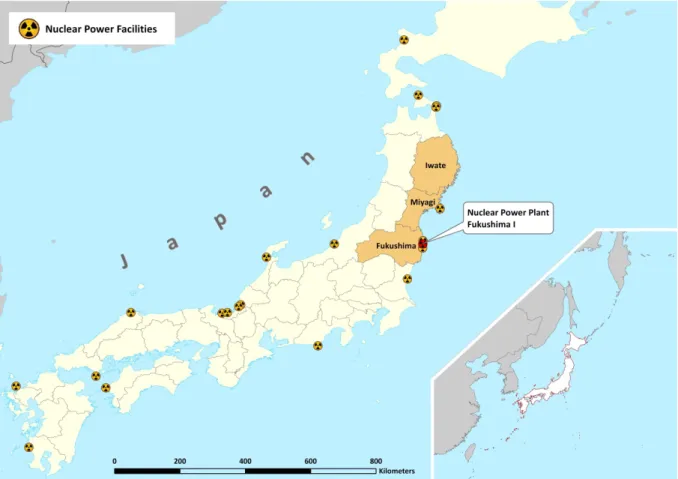
According to the Reconstruction Agency,6 the combined disaster of the earthquake, tsunami, and the nuclear accident caused nearly 16,000 deaths, over 1.2 million destroyed or damaged buildings, temporary evacuation of over 380,000 people from their home, most of whom were residents of Iwate, Miyagi, and Fukushima prefectures on the northeast coast of the Pacific Ocean (see Figure 1). It also disrupted water supply, power distribution, and train, highway and air transport systems in a wide area of eastern Japan. Reconstruction of infrastructures has been partly hindered by radioactive contamination around the nuclear power plant, and as of spring 2013, some key infrastructures, such as a major train line and a major highway (Joban Line and Joban Expressway), have not been recovered yet.
After the nuclear accident, no deaths from radiation exposure have been reported, and long-term radioactivity-related health risks for the Fukushima residents are considered to be low (WHO, 2013). Still, radioactivity added a special dimension to the problem.7 To reduce radiation exposure, all residents approximately within a 20 km radius of the Fukushima Dai-ichi power plant were forced to leave their home.8 Although the surroundings of the Fukushima plant had hardly been a population center or a popular touristic destination, extended periods of evacuation placed severe stress on the evacuees. Due to contamination of radioactive iodine, many local health authorities, including that of Tokyo, 220 km off the Fukushima site, issued recommendations not to give tap water to infants, although most of those warnings were lifted within a month after the disaster. Also, radioactive contamination of farming products was widely detected in Fukushima and the neighboring prefectures.
5
The numbers for Chernobyl are about 10 times larger.
6
http://www.reconstruction.go.jp/topics/000046.html, last accessed on April 5, 2013.
7
Facts presented in the following are according to the Nuclear Emergency Response Headquarters (2011).
8
The number of evacuees from the evacuation zone amounted to approximately 113,000 (estimated by the Cabinet Office in February 2012).
7
Although those products did not enter the market, such cases of contamination economically hurt farmers and also provoked public anxieties about food safety.
Before March 2011, nuclear power had provided about 30% of electricity in Japan, and all the nuclear power plants in the country were gradually suspended after the Fukushima disaster to be given a comprehensive safety test. Supply of electricity was particularly tightened in the summer 2011, a peak season of electricity demand due to the use of air conditioning. Rationing of electricity was placed on large industrial customers (> 500kW), and also the government mounted a large-scale public campaign on conservation of electricity by individual consumers.
Figure 1 displays the distribution and location of the 21 nuclear power stations in Japan, highlighting Fukushima Dai-ichi. The power plants are distributed across the whole country all located at the coast with some clustering.
Figure 1 about here
Social consequences of the disaster, especially those of the nuclear accident, are substantial for the country: for example, there have already been some major changes in energy policy following the event. The Fukushima disaster served as a major impetus to the introduction of a feed-in-tariff scheme for renewable energy, which started in July 2012. The Cabinet also decided in September 2012 that it would not allow any new constructions of nuclear power plants and would phase out all the existing plants by 2030.9
3. Methodology and Data
3.1 General Approach and Empirical Strategy
We use a quasi-experimental difference-in differences (DD) approach to measure the effect of the disaster on SWB, whilst controlling for a range of other factors. The DD design allows us to isolate the effect attributable to the disaster from other contemporaneous variables (e.g. macroeconomic changes), since the control group experiences some or all of the contemporaneous influences that affect SWB in the treatment group without being affected by the event.
9
Although the new government since December 2012 led by the Liberal Democratic Party repeatedly expresses intentions to reconsider the decision (for example, Asahi Shimbun, January 31, 2013, “genpatsu zero, shushou minaosu, shuin daihyou shitsumon”: in Japanese, “the zero nuclear power plants target should be reconsidered, said PM in a Diet interpellation”).
8 The general model employed for this purpose is:
β β β ∗ 1
where SWBijt is the stated subjective well-being of respondent i in location j at time t, Iit is respondent i’s income, Hit represents other socioeconomic and demographic characteristics,
Gjt are region specific information. Ei denotes event variables that indicate whether or to what extent an individual has been affected (treated) by the disaster, Yt is a dummy variable representing the year of the interview. For reasons of data availability (see below), our analysis is restricted to two years, and we set Yt = 1 if the interview took place in the year after the disaster, Yt = 0 otherwise. The symbol ε represents the error term.
The interaction term between the event (treatment) variable and the year of the interview tells us how the disaster might have changed SWB of persons affected by the disaster. It should be noted, however, that we are unable to check common trends in SWB before the event, a key identifying assumption of DD, since we have SWB data only for one year before the event. Within this general framework we estimate a set of different specifications which differ by the way treatment is captured. Among others this includes a measure that identifies which areas were directly affected by the disaster and measures that take into account distance or proximity to the Fukushima site. To identify how severely a region was affected by the disaster we collected information on the number of missing, injured or dead people as well as the number of buildings completely or partly destroyed. This information is available at the level of the municipality.10 While this latter measure (equation 2 below) is more likely to capture the impact of the tsunami caused by the earthquake the distance measures are meant to capture the impact of the nuclear accident (equations 3 and 4 below).
To estimate the impact of the tsunami on SWB we use the following equation:
β β β ∗ 2
10
Data was available from the National Research Institute for Earth Science and Disaster Prevention, http://www.j-risq.bosai.go.jp/ndis, last accessed 20-05-2013)
9
where the key variable of interest, Tj, represents a dummy variable denoting 1 if the individual was living in a municipality being affected by the tsunami and 0 otherwise (Ei = Tj).11 The parameter 4 represents the difference in SWB in the municipalities affected by the tsunami with respect to unaffected municipalities, whilst 5 indicates the difference in SWB in the year after and before the accident. The parameter 6 measures the change (after/before) in SWB in the tsunami regions relative to unaffected regions. Since those regions differ with respect to their location relative to the (unaffected) reference region, 6 is expected to be negative.
Measuring distance we mapped in a first step the location of existing nuclear power stations using GIS (see Figure 1 above).12 Next, we measured the distance of each existing nuclear power station to each municipality.13 Distance to the Fukushima Dai-ichi power station varies between 57 and 1,771 km, being 487 km on average. 14
To estimate the impact of the accident on SWB based on distance measures we use the following equation:
β β β ∗ 3
where the key variable of interest, Dj, represents the distance to the Fukushima Dai-ichi power plant (Ei = Dj). The coefficient of the interaction term of the post-Fukushima dummy with distance to the Fukushima power plant,6, is expected to be positive.
An alternative functional form to capture proximity to the Fukushima site is given by:
β β β β 1 ∗ 4
11
The value is one if dead or injured persons were reported or if destroyed or damaged buildings were reported for the respective municipality.
12
Information on location of existing nuclear power plants was obtained from the National Land Numerical Information Download Service (http://nlftp.mlit.go.jp/ksj-e/gml/gml_datalist.html, last accessed, 29-04-2013).
13
We used the centroid of each municipality.
14
10
This functional form presumes that the effect declines with distance in a hyperbolic fashion (Ei = 1/Dj), whereas the previous formulation involves a linear decay with distance. In this formulation 6 is expected to be negative.
In addition to affecting SWB through its physical consequences, the Fukushima accident may have led to increased worry about nuclear power in general, which may have affected the SWB especially of people living close to nuclear power plants. The corresponding specifications directly follow equations (3) and (4) now measuring distance to the closest existing nuclear power plant instead of Fukushima. Another functional form for the SWB function is the use of count variables to identify the number of nuclear power stations, Z, located in a specific concentric circle with the municipality at the centre e.g. 0-25 km; 0-50 km etc. (Ei = Zj).
In our sample the minimum distance to the closest nuclear power station varies between 18 and 675 km with an average of 124 km. Within a radius of 100 km 68% of the households have at least one nuclear power station, some have up to four.
In estimating these models, SWB will be measured by “happiness with one’s life in the previous year”, which in 2012 refers to the time after the disaster. However, it may be the case that consequences of the tsunami and the nuclear accident influenced people’s assessment not only of their well-being in the year following the event but also of their entire life. To test this hypothesis, we re-estimated some of the above models with “happiness with one’s whole life” as the dependent variable.
3.2 Data
Most of the data used to investigate the well-being effect of the disaster is taken from the KHPS. The KHPS is a representative Japanese household panel conducted by Keio University based on a set of pre-tested questionnaires for both households and individuals. The first wave of KHPS was assembled in 2004 and covered 4,005 households; the most recent one in 2012. The usual sample size ranges between 3,000 and 3,500 households.15 Interviews are always carried out in January.
KHPS provides information on various aspects of the participating individual and the respective households. The questionnaires comprehensively cover information on household
15
For aspects on representativeness of the data see Kimura (2005). For sample attrition in KHPS see Miyauchi et al. (2006), McKenzie et al. (2007), and Naoi (2008).
11
composition, income, occupation, employment history, school attendance, lifestyle and location. In addition to a stable set of core questions, each year the survey focuses on special topics. In 2011 and 2012 the questionnaire included for the first time questions on different aspects of SWB. In order to take advantage of this information and because we are interested in the well-being effects of the accident in March 2011, the analysis relies exclusively on the surveys of 2011 and 2012 (fielded in January of the respective years). Taken together our dataset contains a total number of 5,979 observations. Table A1 in the Appendix provides information on the variables included and the summary statistics.
SWB is measured on an integer scale of 0–10 with an average SWB of 6.24 for our sample when individuals are asked about their happiness referring to the previous year.16 SWB understood as happiness with one’s whole life up to the present, the average of this variable is 6.46.17 Comparing the two SWB measures over time, average SWB decreased from 2011 to 2012 (from 6.25 to 6.23) for the first measure but increased for the second (from 6.45 to 6.47). Explanatory variables, generally found significant in models explaining differences in SWB, are individual characteristics such as age, gender, employment status, education level, and income, number of children, physical condition or marital status. Income enters the regression equation in its natural logarithm to account for declining marginal utility of income.
Controls at the municipality level include population density, the elevation of the municipality as well as latitude and longitude to control for differences in climate.18 At the prefecture level we include information on the rate of unemployment.19 Note that in a macroeconomic sense, the effect of the March 2011 disasters on employment is generally minor.20 To capture further regional differences dummy variables indicate in which of the 47 prefectures the individual is living. A further dummy variable indicates whether observations are drawn from the 2011 or 2012 survey.
16
The exact wording of the question is: Please choose a number on a scale of 0 to 10, where “0” means having no feeling of happiness at all and “10” means fully having a feeling of happiness over the last one year
17
The corresponding question in the KHPS is: Please choose a number on a scale of 0 to 10, for which “0” means having no feeling of happiness at all and “10” means fully having a feeling of happiness for the whole life up to the present.
18
Information on population density was taken from the Population Census. Information on elevation was provided by the National Land Numerical Information Download Service
(http://nlftp.mlit.go.jp/ksj-e/gml/gml_datalist.html, last accessed, 29-04-2013). Elevation, latitude and longitude refer to the centroid of a municipality. There are 1,719 municipalities in total as of January 2013. For 2011 and 2012 KHPS covers 455 municipalities. In our sample the average municipality has a size of about 200 square kilometer.
19
Data was taken from the Labor Force Survey (Ministry of Internal Affairs and Communications of Japan).
20
The number of job seekers in the three most affected prefectures (Fukushima, Miyagi, Iwate: the total population is about 5.7 million) peaked at about 164,000 in June 2011 but declined afterwards (Ministry of Health, Labor and Welfare, http://www.mhlw.go.jp/stf/houdou/2r9852000001z9f4.html, last accessed on May 24, 2013).,
12 4. Results
Based on the results by Ferrer-i-Carbonell and Frijters (2004) our empirical analysis uses OLS. In order to account for the possible correlation of residuals when observations are taken from the same individual over time, we report robust standard errors. The effect is to increase the standard errors of the parameter coefficients. This procedure also leads to robust variance estimates in the face of heteroskedasticity.
4.1 Basic Results
Table 1 presents the results of the first two model specifications using SWB as referring to the previous year as the dependent variable. Model 1 is a truncated version of equation (1) which omits the event variables, variables Ei and Ei * Yi..
Table 1 about here
Results of Model 1 confirm those of earlier studies using data from other countries (see, e.g., Dolan et al. 2008). Consistent with earlier analyses we find a U-shaped relationship with age21 and a positive and diminishing marginal utility of income. Unemployed, sick and single individuals are significantly less happy than their counterparts. Individuals with higher levels of education or those currently being in education are happier as well as those being in retirement or those doing housekeeping or taking care of the kids. The presence of children has no significant effect on SWB but the size of the household has. It is negative. Being a male effects SWB negatively. Turning to the geographical variables; people living in Kanagawa, a highly populated prefecture close to Tokyo, seem to be happier than those in the reference region (Iwate, Miyagi and Fukushima). The coefficient is significant only at the 10 percent level of confidence (results for prefectures are not presented individually). All other variables are statistically not significant. Comparing observations from the 2011 survey to the 2012 survey reveals no significant difference.
The results of Model 2 (equation 2), also presented in Table 1, indicate that before the accident SWB in the areas affected by the tsunami was not significantly different from those
21
13
in other areas. The interaction effect, however, is negative, as expected and statistically significant. Post-Fukushima location mattered: individuals located in areas not directly affected by the tsunami experienced higher SWB. The F-statistic of joint significance of T and Y*T, however, results in a P-value of 0.1003 only. The other results are comparable to those of Model 1.
Turning to the results of the Models capturing distance to the Fukushima site, results of Model 3 (equation 3) suggest that before the accident distance to the Fukushima site had no statistically significant effect on people’s SWB. The interaction effect, however, is positive, as expected, and statistically significant. Post-Fukushima the distance to the power plant mattered: individuals experienced higher SWB the more distant from the place of the accident they lived. Looking at results for Model 4, the inverse distance specification (equation 4), we find a statistically significant effect on SWB before and after the accident. The estimated coefficient is positive before the accident and, as expected, negative after the accident. The other results are comparable to those of Model 1. The positive coefficient could be a reflection of strong economic standings of the areas around the Fukushima site before the accident, which seems to be better captured by the hyperbolic than by the linear specification.22
4.2 Valuing the treatment effect
To investigate the treatment effect (parameter 6 in equations (1) to (4)), the DD-estimator can be written as (Meyer 1995):
, , , , 5
The parameter 6 would be statistically not different from zero, if we assume that in the absence of the disaster SWB would have changed identically in the treatment group T and the control group C. Our results suggest otherwise
22
In Japan, surrounding areas of nuclear power plants enjoy various economic benefits, such as the subsidies based on the Power Source Siting Laws (dengen san pou) and large property tax revenues from the siting power company. Also, the power company and related businesses tend to constitute a dominant proportion of the local economy around a nuclear power plant. For example, before the Fukushima accident, more than 60% of the economic output in the Futaba county (where the Fukushima Dai-ichi power plant is located) was electricity related (source: the Reconstruction Agency website,
14
We now use our results to compute the amount a person would be willing to pay to avoid being treated. To this purpose we convert the treatment effect in equation (5), which is measured in units of SWB, into monetary units by dividing it by / , where M denotes income (with I = lnM).23
Results of Model 2 suggest that the monetary equivalent for a household with average income is about ¥ 3,700,000 to avoid living in a municipality affected by the tsunami. This corresponds to 72 percent of annual average income. Post-Fukushima the treatment effect for a one kilometer increase in distance from the Fukushima site is ¥ 6,800 for the average household (Model 3).24 Applying results of Model 4 numbers are about ¥ 5,000 for mean distance (487 km); about ¥ 340,000 for minimum (57 km) and about ¥ 350 for maximum (1771 km) distance. The figure of ¥ 340,000 for a move from 57 km (minimum distance) to 58 km from the Fukushima site corresponds to 6.6 percent of average income. For a non-marginal change in distance, e.g. from minimum distance to a distance of 100 km, the compensating surplus for the same household is about ¥ 1,015,000 or 20 percent of income. The results are comparable, although at the higher end, to those of others investigating other single events. Lüchinger and Raschky (2009), for example, calculate an average WTP of one sure flood event in the region of residence corresponding to 24 percent of an average household income. Caroll et al. (2009) calculated that a drought in Australia is equivalent to an income loss of 38 percent for a household with mean household income.
4.3 Extensions
The first extension relates to the hypothesis that, in addition to being affected by the physical consequences of the disaster, well-being is influenced by increased worry about nuclear power among those living close to nuclear power plants or by the number of nuclear power stations in the vicinity. According to Models 5 to 10 (Table 2), distance to or presence of nuclear power stations in general is mostly insignificant. An exception is Model 9 where the number of nuclear power stations within a distance of 75 km has a significant effect on SWB, but the coefficient is significant only at the 10 percent level and the F-statistic of joint significance of Y and Z*Y results in a P-value of 0.1633.
23
Formally, this way we compute the marginal rate of substitution of income for treatment.
24
The average net household income in our sample is ¥ 5,100,000 (evaluated with the average exchange rate of January 2012, ¥ 100 is worth US$ 1.30).
15
Table 2 about here
The second extension relates to our dependent variable, which up to this point was people’s happiness in the year before the respective interview. In the following we analyze if the accident has an effect on SWB understood as happiness with one’s whole life up to the present. Table 3 presents results of specifications equivalent to Models 1 to 4, where the replacement of the dependent variable is the only difference. Comparing the results to those presented in Table 1 we find no change in sign and significance of most variables previously included. An important exception is the pre-Fukushima effect. In all three models, Models 2a to 4a, we find no statistically significant effect for the respective variables.25 In Model 4a the F-statistic on joint significance of Y and (1/D)*Y results in a P-value of 0.0181. Another difference is the insignificant effect of unemployment. Though the accident seems to have affected people’s evaluation of the quality of their lives after the event, it has not influenced their assessment of their life as a whole.
Table 3 about here
4.4 Robustness Checks
Finally, we test whether our results are robust to alternative specifications (results are not presented). Replacing the distance measures by a variable measuring the distribution of radioactive substances across municipalities, we analyze the effect of air dose rate on SWB. By doing so, we account for the fact that the prevailing wind direction after the accident affected regions close to Fukushima very differently. A distance measure would not be able to pick this up. The new variables are not individually nor jointly significant at the 10% level of confidence (F (2,5902)=0.25, P=0.7824).26
Further, when replacing the tsunami dummy, T in equation (2), by a dummy with value one if dead persons were reported in the respective municipality, the results are comparable to those
25
This is true for the other model specifications as well which are not presented here.
26
Information is taken from the Database on the Research of Radioactive Substances Distribution provided by the Ministry of Education, Culture, Sports, Science and Technology (http://radb.jaea.go.jp/mapdb/en/). The average of total cesium-134 and -137 depositions per municipality on April 29, 2011 was used. This is the earliest day after the accident for which data of wide-scale airborne measurements are available.
16
of Model 2 with a slightly higher 6-coefficient (-0.4101). When replacing the tsunami dummy with a dummy indicating if buildings were completely destroyed in the respective municipality, the coefficient 6 is smaller (-0.0001). In both cases, the new variables are individually and jointly significant. So far, we have not considered the possibility of selection bias, that is, people most seriously suffering from the event refused to participate in the 2012 round of the survey. In addition, given that all residents within a certain radius from the Fukushima Dai-ichi power plant were evacuated to more distant places after the event, it is likely that the location of some of the interviewees as of 2012 was more distant than it was at the time of the disaster. This relocation effect may introduce a downward bias into the relationship between distance and the change in SWB. Both the selection and the relocation effect, if present, will lead to a downward bias in our estimates of the well-being effect of the Fukushima disaster. Further, people that lived in the affected areas or closer to Fukushima before the disaster are perhaps more likely to get unemployed or to have health related problems.
When omitting the variables measuring income, health and presence of unemployment from Model 4, results of the remaining variables are robust. The variables measuring the inverse distance to the Fukushima site (Prox_Fukushima) are still highly significant, the coefficient of the interaction term 2012*Prox_Fukushima gets a bit smaller (-73.66 compared to -80.41 in Model 4). 27 Similar results are obtained when restricting the sample to those individuals that participated in both years in the KEIO panel. Restricting the sample further by excluding those that moved does not change the results.28 Next, including a term interacting unemployment and inverse distance to the Fukushima site to test if unemployed persons closer to Fukushima show lower levels of SWB, the term has the expected negative sign and is significant at the 5% level.29 Finally, including a term interacting health status and inverse distance to the Fukushima site we test if individuals that report lower levels of health status are unhappier if they live closer to the Fukushima site. The term is positive, as expected, and significant at the 5% level confirming the hypothesis. 30 Other results are unchanged.
27
F(2, 5907)=7.18, P=0.0008.
28
In general, few individuals moved between the two survey years (only 30) and no regional pattern is observable. The drop-out rate between the 2011 and 2012 samples shows no bias towards locations that were more heavily affected. It reduces our sample to 5,008 observations. Also, the 2011 KEIO samples include no households located in the evacuation zone.
29
F-Text on joint significance of Unemployed + Unemployed*Prox_Fukushima results in F(2,4860)=5.20, P=0.0056.
30
We tried both; health measured as categorical variables as in Model 5 and as a continuous variable. The F-test for the specification with the continuous variable (Health + Health* Prox_Fukushima) resulted in F(2,
17
Combined, irrespective of the robustness checks we perform the interaction term of post-Fukushima dummy and inverse distance is negative and highly significant.
5. Discussion and Conclusion
Using data from KHSP, we conducted for the first time a quasi-experimental SWB study of the combined disaster of an earthquake, tsunami and a nuclear accident near Fukushima on March 11, 2011 taking into account the spatial dimension.
With regard to the factors of SWB we found evidence highly consistent with findings from Western countries in spite of differences in the cultural background.31 The plausibility of those results enhances our confidence in the suitability of the KHSP database for studying the main issue of this paper, the effects of the Fukushima events on SWB. Possible SWB effects of Fukushima relate, in the first place, to the physical consequences of the disaster (in particular fatalities to relatives and friends, destruction of buildings and infrastructures, release of radiation, evacuation of residents, shortage of basic necessities such as electricity and water). In the second place, it is conceivable that people’s well-being dropped even if not directly affected due to increased worry about nuclear power. Finally, for those most seriously affected by the disaster it could be that not only the assessment of their happiness after the event deteriorated, but also their assessment of their entire life.
One main finding from our empirical analysis is a significant drop in SWB after the disaster in places affected by the tsunami but not elsewhere. Another one is a significant drop in SWB proportional to proximity to the place of the nuclear accident, the Fukushima Dai-ichi nuclear power plant. This result is robust to a number of robustness checks. In particular, it is not affected by selection bias or relocation bias. Given that the physical effects of the nuclear accident decay with distance, we take this as evidence of an effect of the nuclear disaster on SWB. In our preferred specification we assume that the effect size decreases with distance in a hyperbolic fashion. Based on this model, we find the monetary equivalent of a 1-km increase in distance to the Fukushima site to be about ¥ 6,800 for a household with average income at mean distance. For a household at minimum distance to the Fukushima nuclear plant, which is 57 km, the monetary equivalent of a 1-km increase in distance is about ¥ 340,000 or 6.6 percent of average annual income. The monetary equivalent goes to up to 72
31
Culture-specific and unique characteristics to Japan or East Asia, originating from either prevailing
philosophical traditions (e.g., Buddhism) or traits of collectivism are still present in Japan despite ongoing shifts towards individualism due to globalization. For a review see Tov and Diener (2007) and Uchida and Ogihara (2012).
18
percent of annual average income for those living in affected regions. These numbers are comparable at the higher end to those of others analyzing other single events, like floods and droughts.
In interpreting these results it should be noted that the underlying regressions control for income, the employment status, and the health status. Therefore, the above figures represent the intangible effects in the strictest sense, that is, disregarding effects from lost jobs, reduced income, and sickness, all of which contribute to SWB in a statistically and substantively significant way.
In contrast to the physically-based effects on SWB we find no evidence of a psychological effect in terms of increased worry about nuclear power for those living close to nuclear power plants. However, this lack of an effect is plausible because all the nuclear power plants in the country were suspended after the Fukushima disaster. Therefore, this finding lends additional credibility to our approach and findings rather than discrediting them.32
Finally, in spite of the significant and sizeable effects on SWB after the disasters, people’s assessments of the quality of their entire life do not seem to have been affected by them. This might be explained by the philosophical traditions influential in East Asia (e.g., Buddhism and Daoism) emphasizing the dialectic nature of things, and East Asians in fact have relatively accepting attitudes towards negative emotions and events. This also relates to how East Asians regard happiness. For example, Uchida and Kitayama (2009) find that the Japanese participants in their experiment tend to associate happiness even with some negative features, such as jealousy from others and inattention to one’s surroundings, and that this result is in contrast to that of the American participants of the experiment, whose view of happiness tends to be entirely positive.
As to the limitations of this study, we are able to measure short-run effects only. This may explain why we found no effects of the level of radiation, as these effects may be of a more long-term character.
Acknowledgement
We would like to thank Swantje Sundt and Tim Hartmann for outstanding research assistance and Susana Ferreira and Arik Levinson for insightful comments. The data analysis in this
32
As of May 2013, 48 out of 50 commercial nuclear reactors in Japan are still suspended or are to be decommissioned.
19
paper utilizes Keio Household Panel Survey (KHPS) data provided by the Panel Data Research Center at Keio University. The Excellence Initiative Future Ocean provided welcome financial support. The usual disclaimer applies.
References
Almond, D., Edlund, L., Palme, M. (2009), Chernobyl’s subclinical legacy: Prenatal exposure to radioactive fallout and school outcomes in Sweden, Quarterly Journal of Economics, 1729-1772.
Berger, E.M. (2010), The Chernobyl Disaster, Concern about the Environment, and Life Satisfaction, Kyklos 63, 1-8.
Carroll, N., Frijters, P., Shields, M.A. (2009), Quantifying the Costs of Drought: New Evidence from Life Satisfaction Data, Journal of Population Economics 22, 445-461. Clark, A.E., Frijters, P., Shields, M.A. (2008), Relative Income, Happiness and Utility: An
Explanation for the Easterlin Paradox and Other Puzzles, Journal of Economic Literature 46, 95-144.
Diener, E., Suh, E.M., Lucas, R.E., Smith, H.L. (1999), Subjective Well-Being: Three Decades of Progress, Psychological Bulletin 125, 276-302.
Di Tella, R., MacCulloch, R., Oswald, A. (2001), Preferences over Inflation and Unemployment: Evidence from Surveys of Happiness, American Economic Review 91, 335-341.
Dolan, P., Peasgood, T., White, M. (2008). “Do we really know what makes us happy? A review of the economic literature on the factors associated with subjective well-being”,
Journal of Economic Psychology 29, 94-122.
Ferreira, S., Moro, M. (2010), On the Use of Subjective Well-Being Data for Environmental Valuation, Environmental and Resource Economics, 46 249-273.
Ferrer-i-Carbonell, A., Frijters, P. (2004), How Important is Methodology for the Estimates of the Determinants of Happiness?, Economic Journal 114, 641-659.
Frey, B.S., Stutzer, A (2000), Happiness, Economy and Institutions, Economic Journal 110, 918-938.
20
Frey, B.S., Stutzer, A. (2002), What Can Economists Learn from Happiness Research?,
Journal of Economic Literature 40, 402-435.
Frey, B.S., Luechinger, S., Stutzer, A. (2009), The Life Satisfaction Approach to Valuing Public Goods: The Case of Terrorism, Public Choice 138, 317-345.
Kahneman, D. Wakker, P.P., Sarin, R. (1997), Back to Bentham? Explorations of Experienced Utility, Quarterly Journal of Economics 112, 375-405.
Kimball, M.,Levy, H., Ohtake, F., Tsutsui, Y (2006) Unhappiness after hurricane Katrina, NBER Working Paper 12062, Cambridge.
Kimura, M. (2005), The Sample Characteristics of the 2004 Keio Household Panel Survey (2004nen Keio Gijuku Kakei Paneru Chosa no Hyohon Tokusei), chapter 1 in Y. Higuchi (ed.), Dynamism of Household Behavior in Japan [I] (Nihon no Kakei Kodo no Dainamizumu [I]), Keio University Press, Tokyo, 13-41 (in Japanese).
Levinson, A. (2012), Valuing public goods using happiness data: The case of air quality,
Journal of Public Economics 96(9-10), 869-880.
Luechinger, S. (2009), Valuing Air Quality Using the Life Satisfaction Approach, Economic
Journal 119, 482-515
Luechinger, S., Raschky, P.A. (2009), Valuing Flood Disasters Using the Life Satisfaction Approach, Journal of Public Economics 93, 620-633.
McKenzie, C.R., Miyauchi, T., Naoi, M., Kiso, K. (2007), Individual Behaviour and the Attrition Problem in the Labour Market (Rodo Shijo ni okeru Kojin Kodo to Datsuraku Mondai), chapter 1 in Y. Higuchi and M. Seko (eds), Dynamism of Household Behavior in Japan[II] (Nihon no Kakei Kodo no Dainamizumu [III]), Keio University Press, Tokyo, 13-75 (in Japanese).
MacKerron, G. (2012), Happiness economics from 35 000 feet, Journal of Economic Surveys 26, 705-735.
MacKerron, G., Mourato, S. (2009), Life Satisfaction and Air Quality in London, Ecological
Economics 68, 1441-1453.
Maddison, D., Rehdanz, K. (2011), The Impact of Climate on Life Satisfaction, Ecological
21
Metcalfe, R., Powdthavee, N., Dolan, P. (2011), Destruction and Distress: Using a Quasi-Experiment to Show the Effects of the September 11 Attacks on Mental Well-Being in the United Kingdom, Economic Journal 121, F81-F103.
Meyer, B.D. (1995), Natural and Quasi-Experiments in Economics, Journal of Business ans
Economic Statistics 13, 151-161.
Miyauchi, T., McKenzie, C.R., Kimura, M. (2006), An Analysis of Panel Data Continuation and Responses (Paneru Deta Keizoku to Kaito Bunseki), chapter 1 in Y. Higuchi (ed.), Dynamism of Household Behavior in Japan [II] (Nihon no Kakei Kodo no Dainamizumu [II]), Keio University Press, Tokyo, 9-52 (in Japanese).
Murray, T., Maddison, D., Rehdanz, R. (2013), Do Geographical Variations in Climate Influence Life Satisfaction? Climate Change Economics 4 (1), DOI: 10.1142/S2010007813500048.
Naoi, M. (2008), Residential Mobility and Panel Attrition: Using the Interview Process As Identifying Instruments, Keio Economic Studies 44(1), 37-47.
Rehdanz, K., Maddison, D. (2005), Climate and Happiness, Ecological Economics 52, 111-125.
Seko, M., Teruyama, H., Yamamoto, I., Higuchi, Y. and Keio/Kyoto Joint Global Center of Excellence Program (eds.) (2012), Higashi Nihon Daishinsai ga kakei ni Ataeta Eikyo (The Impacts of East Japan Earthquake on Household) , Tokyo: Keio University Press.
Seko, M., Teruyama, H., Yamamoto, I., Higuchi, Y. and Keio/Kyoto Joint Global Center of Excellence Program (eds.) (2013), Kakei Paneru deta kara mita shijou no shitu (Market Quality in Household Panel Survey Data), Tokyo: Keio University Press.
Tov, W. and Diener, E. (2007), Culture and Subjective Well-Weing, in S. Kitayama and Cohen, D. (Eds.), Handbook of Cultural Psychology, pp. 691-713, New York, Guilford. Uchida, Y. and Kitayama, S. (2009), Happiness and Unhappiness in East and West: Themes
and Variations, Emotion 9, 441-456.
Uchida, Y. and Ogihara, Y. (2012), Personal or Interpersonal Construal of Happiness: A Cultural Psychological Perspective, International Journal of Wellbeing 2(4), 354-369. Van Praag, B., Baarsma, B. (2005) Using Happiness Surveys to Value Intangibles: The Case
22
Van Praag, B.M.S., Ferrer-i-Carbonell, A., 2008. Happiness Quantified: A Satisfaction Calculus Approach, Oxford University Press.
Welsch, H. (2002), Preferences over Prosperity and Pollution: Environmental Valuation Based on Happiness Surveys, Kyklos 55, 473-494.
Welsch, H. (2006), Environment and Happiness: Valuation of Air Pollution Using Life Satisfaction Data, Ecological Economics 58, 801-813.
Welsch, H. (2008a), The Social Costs of Civil Conflict: Evidence from Surveys of Happiness,
Kyklos 61, 320-340.
Welsch, H. (2008b), The Welfare Costs of Corruption, Applied Economics 40, 1839-1849. Welsch, H., Kühling, J. (2009), Using Happiness Data for Environmental Valuation: Issues
23 Table 1: Regression results
Model 1 Model 2 Model 3 Model 4
Coefficient Standard Error Coefficient Standard Error Coefficient Standard Error Coefficient Standard Error
Individual Information Income 0.3699 0.0477 *** 0.3707 0.0476 *** 0.3725 0.0476 *** 0.3724 0.0476 *** Age -0.0701 0.0176 *** -0.0710 0.0176 *** -0.0712 0.0176 *** -0.0700 0.0176 *** Age (squared) 0.0008 0.0002 *** 0.0008 0.0002 *** 0.0008 0.0002 *** 0.0008 0.0002 *** Male -0.2994 0.0621 *** -0.2938 0.0620 *** -0.2969 0.0620 *** -0.2923 0.0620 *** Size -0.1257 0.0279 *** -0.1245 0.0279 *** -0.1242 0.0279 *** -0.1229 0.0279 ***
Single (reference category) (reference category) (reference category) (reference category)
Married 0.8526 0.0879 *** 0.8508 0.0879 *** 0.8504 0.0879 *** 0.8523 0.0878 ***
Other 0.0035 0.2028 0.0035 0.2019 0.0014 0.2012 0.0075 0.2012
Children 0.0531 0.0378 0.0531 0.0378 0.0536 0.0378 0.0521 0.0378
Edulevel 1 (reference category) (reference category) (reference category) (reference category)
Edulevel 2 0.1992 0.1206 * 0.1988 0.1206 * 0.1955 0.1207 0.1950 0.1199 Edulevel 3 0.2674 0.1438 * 0.2663 0.1437 * 0.2610 0.1436 * 0.2652 0.1431 * Edulevel 4 0.3976 0.1324 *** 0.3911 0.1324 *** 0.3876 0.1324 *** 0.3897 0.1318 *** Edulevel 5 -0.0286 0.2746 -0.0396 0.2752 -0.0417 0.2747 -0.0367 0.2743 Edulevel 6 0.4634 0.1355 *** 0.4611 0.1356 *** 0.4590 0.1355 *** 0.4638 0.1350 *** Edulevel 7 -0.2257 0.2329 -0.2341 0.2319 -0.2373 0.2323 -0.2339 0.2326
Employed (reference category) (reference category) (reference category) (reference category)
Student 0.8526 0.3268 *** 0.8518 0.3273 *** 0.8490 0.3280 *** 0.8527 0.3281 ***
Retired 0.2227 0.1167 ** 0.2109 0.1163 * 0.2095 0.1165 * 0.2033 0.1162 *
Unemployed -0.6305 0.2241 *** -0.6230 0.2251 *** -0.6161 0.2257 *** -0.6144 0.2253 ***
Home 0.1910 0.0812 ** 0.1945 0.0810 ** 0.1892 0.0811 ** 0.1905 0.0811 **
Health 1 (reference category) (reference category) (reference category) (reference category)
Health 2 -0.6767 0.0918 *** -0.6720 0.0918 *** -0.6748 0.0917 *** -0.6721 0.0917 ***
Health 3 -1.4563 0.0897 *** -1.4529 0.0898 *** -1.4572 0.0898 *** -1.4539 0.0896 ***
24
Health 5 -3.4212 0.3520 *** -3.4052 0.3501 *** -3.4063 0.3509 *** -3.3846 0.3513 ***
Geographical and other information
Tsunami 0.1123 0.1292 2012*Tsunami -0.2682 0.1267 ** Fukushima -0.0008 0.0010 2012*Fukushima 0.0005 0.0002 *** FukushimaInv 178.2727 58.2195 *** 2012*FukushimaInv -80.4063 23.1874 *** Unemployment -0.1104 0.1966 -0.1068 0.2237 -0.0015 0.2189 -0.1857 0.2242
Popdens 0.0000 0.0000 1.40E-06 9.30E-06 3.54E-07 9.39E-06 -3.85E-07 9.32E-06
Elevation 0.0000 0.0002 -0.0001 0.0002 -0.0001 0.0002 -0.0001 0.0002 Longitude -0.0803 0.1034 -0.0930 0.1036 -0.0952 0.1041 -0.1278 0.1046 Latitude 0.0769 0.1132 0.2510 0.1262 ** 0.2736 0.1316 ** 0.2706 0.1263 ** 2012 11.3031 13.0449 0.0158 0.0822 -0.2676 0.1156 ** 0.1769 0.0995 * Constant -0.1104 0.1966 9.3430 12.2892 9.4249 12.4856 13.5903 12.3956
Region YES YES YES YES
R2 0.1804 0.1821 0.1827 0.1839
F-Test (P>F) 0.1008* 0.0155** 0.0002***
N 5979 5979 5979 5979
Note: Significance at the ten-percent level is indicated by *, significance at the five-percent level is indicated by ** and significance at the one-percent level is indicated by ***.
a
Reported are robust standard errors.
b
25 Table 2: Alternative specifications
Model 5 Model 6 Model 7 Model 8 Model 9 Model 10
Coefficient Coefficient Coefficient Coefficient Coefficient Coefficient Individual Information Income 0.3707 *** 0.3687 *** 0.3686 *** 0.3690 *** 0.3704 *** 0.3696 *** Age -0.0709 *** -0.0705 *** -0.0708 *** -0.0716 *** -0.0702 *** -0.0713 *** Age (squared) 0.0008 *** 0.0008 *** 0.0008 *** 0.0008 *** 0.0008 *** 0.0008 *** Male -0.2951 *** -0.2932 *** -0.2925 *** -0.2945 *** -0.2949 *** -0.2951 *** Size -0.1236 *** -0.1237 *** -0.1237 *** -0.1239 *** -0.1235 *** -0.1246 ***
Single (reference category)
Married 0.8525 *** 0.8500 *** 0.8488 *** 0.8492 *** 0.8528 *** 0.8495 ***
Other -0.0037 -0.0039 -0.0008 0.0021 -0.0044 -0.0023
Children 0.0532 0.0530 0.0532 0.0532 0.0518 0.0539
Edulevel 1 (reference category)
Edulevel 2 0.1897 0.1952 0.1986 0.2006 * 0.1902 0.1966 Edulevel 3 0.2570 * 0.2630 * 0.2671 * 0.2685 * 0.2531 * 0.2636 * Edulevel 4 0.3797 *** 0.3875 *** 0.3923 *** 0.3960 *** 0.3784 *** 0.3866 *** Edulevel 5 -0.0410 -0.0318 -0.0320 -0.0399 -0.0349 -0.0327 Edulevel 6 0.4530 *** 0.4584 *** 0.4611 *** 0.4634 *** 0.4528 *** 0.4589 *** Edulevel 7 -0.2360 -0.2353 -0.2318 -0.2236 -0.2532 -0.2384
Employed (reference category)
Student 0.8546 *** 0.8579 *** 0.8561 *** 0.8551 *** 0.8647 *** 0.8599 *** Retired 0.2146 * 0.2152 * 0.2153 * 0.2130 * 0.2159 * 0.2138 * Unemployed -0.6143 *** -0.6190 *** -0.6228 *** -0.6226 *** -0.6140 *** -0.6162 *** Home 0.1931 ** 0.1942 ** 0.1956 ** 0.1931 ** 0.1922 ** 0.1922 **
Health 1 (reference category)
26
Health 3 -1.4539 *** -1.4517 *** -1.4534 *** -1.4570 *** -1.4536 *** -1.4563 *** Health 4 -2.2904 *** -2.2885 *** -2.2911 *** -2.2949 *** -2.2876 *** -2.2930 *** Health 5 -3.4010 *** -3.3937 *** -3.3986 *** -3.4100 *** -3.3950 *** -3.3997 *** geographical and other information
Nuclear -0.0024 2012*Nuclear 0.0002 NuclearInv 8.2069 2012*NuclearInv -1.8816 Nuclear 25 0.2618 2012*Nuclear25 -0.1170 Nuclear 50 -0.1410 2012*Nuclear50 0.0055 Nuclear 75 0.1435 * 2012*Nuclear75 -0.0085 Nuclear 100 0.0152 2012*Nuclear100 0.0529 Unemployment -0.0114 -0.0012 0.0041 -0.0004 0.0020 -0.0071
Popdens 1.90E-06 1.36E-06 1.43E-06 7.53E-07 1.02E-06 6.55E-08
Elevation -0.0001 -0.0001 -0.0001 -0.0001 -0.0001 -0.0001
Longitude 0.0174 -0.0645 -0.0849 -0.1058 -0.0678 -0.0864
Latitude 0.2453 * 0.2481 * 0.2494 * 0.2631 * 0.2519 * 0.2505 *
2012 -0.0554 -0.0061 -0.0230 -0.0263 -0.0218 -0.0634
Constant -3.7719 5.0483 7.6133 9.9877 5.3442 7.8924
Region YES YES YES YES YES YES
R2 0.1818 0.1816 0.1816 0.1817 0.1819 0.1817
F-Test (P>) 0.3121 0.5472 0.7224 0.5087 0.1633 0.3889
N 5,979 5,979 5,979 5,979 5,979 5,979
Note: Significance at the ten-percent level is indicated by *, significance at the five-percent level is indicated by ** and significance at the one-percent level is indicated by ***.
a
27 Table 3: Alternative dependent variable
Model 1a Model 2a Model 3a Model 4a Coefficient Coefficient Coefficient Coefficient Individual Information Income 0.3868 *** 0.3876 *** 0.3873 *** 0.3884 *** Age -0.0563 *** -0.0563 *** -0.0563 *** -0.0549 *** Age (squared) 0.0006 *** 0.0006 *** 0.0006 *** 0.0006 *** Male -0.2510 *** -0.2510 *** -0.2514 *** -0.2481 *** Size -0.0978 *** -0.0980 *** -0.0978 *** -0.0964 ***
Single (reference category)
Married 0.7418 *** 0.7423 *** 0.7419 *** 0.7440 *** Other 0.1108 0.1131 0.1110 0.1150 Children 0.0662 * 0.0660 * 0.0663 * 0.0651 * Edulevel 1 (reference category)
Edulevel 2 0.2699 ** 0.2691 ** 0.2693 ** 0.2649 ** Edulevel 3 0.4643 *** 0.4628 *** 0.4633 *** 0.4619 *** Edulevel 4 0.6704 *** 0.6687 *** 0.6695 *** 0.6667 *** Edulevel 5 0.5581 ** 0.5550 ** 0.5568 *** 0.5533 ** Edulevel 6 0.6366 *** 0.6349 *** 0.6360 *** 0.6368 *** Edulevel 7 -0.0753 -0.0753 -0.0762 -0.0751
Employed (reference category)
Student 0.8922 *** 0.8878 *** 0.8911 *** 0.8904 *** Retired 0.1413 0.1407 0.1408 0.1356 Unemployed -0.2368 -0.2384 -0.2363 -0.2317 Home 0.1469 ** 0.1472 ** 0.1463 ** 0.1454 ** Health 1 (reference category)
Health 2 -0.4748 *** -0.4748 *** -0.4753 *** -0.4727 *** Health 3 -1.1340 *** -1.1334 *** -1.1344 *** -1.1319 *** Health 4 -1.6156 *** -1.6150 *** -1.6166 *** -1.6160 *** Health 5 -2.4292 *** -2.4279 *** -2.4300 *** -2.4146 *** Geographical and other information
Tsunami 0.0015 2012*Tsunami -0.0802 Fukushima -0.0001 2012*Fukushima 0.0001 FukushimaInv 144.0957 *** 2012*FukushimaInv -12.0343 Unemployment -0.0694 -0.1023 -0.0701 -0.1070 Popdens 1.11E-05 1.13E-05 1.10E-05 9.48E-06 Elevation 4.54E-05 4.34E-05 4.41E-05 5.82E-05 Longitude -0.0806 -0.0790 -0.0807 -0.1147 Latitude 0.1977 * 0.1957 * 0.2004 * 0.2205 * 2012 -0.0205 -0.0082 -0.0589 0.0077 Constant 6.0541 7.9859 8.0456 11.7842
Region YES YES YES YES
28
F-Test (P>F) 0.7214 0.8810 0.0181 **
N 5979 5979 5979 5979
Note: Significance at the ten-percent level is indicated by *, significance at the five-percent level is indicated by ** and significance at the one-percent level is indicated by ***.
a
29
Figure 1: Distribution and location of nuclear power plants in Japan
30
Appendix Table A1: Definition of variables and summary statistics
Variable Definition Mean Std. Dev. Min Max
Individual information Happy (last
year)
Average score of self-reported happiness on a 0-10 scale
6.2429 2.2487 0 10
Happy (whole life)
Average score of self-reported happiness on a 0-10 scale
6.4593 2.0234 0 10
Income Logarithm of annual household net income (in 10,000 ¥)
15.2556 0.6546 11.16 18.04
Age Age of the individual 52.1500 13.2683 20 78 Male Unity if individual is a male, zero
otherwise
0.4902 0.4999 0 1
Size Size of household 3.2838 1.4489 1 10 Single Unity of individual is a single, zero
otherwise
0.1980 0.3985 0 1
Married Unity if individual is married, zero otherwise
0.7764 0.4167 0 1
Other Unity if individual is divorced or married, zero otherwise
0.0256 0.1579 0 1
Children number of children living in household 1.1387 1.1223 0 7 Edulevel 1 Unity if individual has a jr. high school
degree, zero otherwise
0.0674 0.2507 0 1
Edulevel 2 Unity if individual has a high school degree, zero otherwise
0.4073 0.4914 0 1
Edulevel 3 Unity if individual has a jr. college or technical college degree, zero otherwise
0.1193 0.3241 0 1
Edulevel 4 Unity if individual has an university degree, zero otherwise
0.1845 0.3879 0 1
Edulevel 5 Unity if individual has a graduate school degree, zero otherwise
0.0134 0.1149 0 1
Edulevel 6 Unity if individual has another degree, zero otherwise
0.1800 0.3842 0 1
Edulevel 7 Unity if individual has no degree, zero otherwise
0.0202 0.1408 0 1
Employed Unity if individual is employed (including self-employment), zero otherwise
0.7461 0 1
Student Unity if individual is a in education, zero otherwise
0.0080 0.0892 0 1
Retired Unity if individual is retired, zero otherwise
0.0641 0.2449 0 1
Unemployed Unity if individual is unemployed, zero otherwise
0.0187 0.1356 0 1
Home Unity if individual is
housekeeping/childraising, zero otherwise
0.1631 0.3695 0 1
Health 1 Unity if individual has a good health status, zero otherwise
0.1253 0.3311 0 1
Health 2 Unity if individual has a pretty good health status, zero otherwise
0.2893 0.4535 0 1
Health 3 Unity if individual has a normal health status, zero otherwise
0.4385 0.4962 0 1
Health 4 Unity if individual has a not so good health status, zero otherwise
0.1351 0.3419 0 1
Health 5 Unity if individual has a bad health status, zero otherwise
0.0117 0.1076 0 1
31
Unemployment Rate of unemployment (%) 4.6283 0.7678 2.2 7.6 Popdens Population density in persons per square
kilometer
4198.6820 4927.4170 5.9 21881.5
Elevation in m 106.7725 177.8110 0 1374 Longitude in ° 137.0974 3.3778 127.69 144.28 Latitude in ° 35.5988 2.3850 26.15 44.31 Tsunami Unity if individual is living in a
municipality affected by the tsunami, zero otherwise
0.2587 0.4380 0 1
Nuclear Minimum distance to next operating nucelar power plant (km)
124.1223 75.0379 18 675
NuclearInv Inverse minimum distance to next operating nucelar power plant (km)
0.0107 0.0069 0.0015 0.0564
Dist_Fukushima Distance to Fukushima I (km) 487.1440 308.9464 57 1771 Prox_Fukushima Inverse Distance to Fukushima I (km-1) 0.0031 0.0023 0.0006 0.0174 Nuclear 25 25 km radius (Number of nuclear power
plants in a radius of 25 km)
0.0144 0.1191 0 1
Nuclear 50 50 km radius (Number of nuclear power plants in a radius of 50 km)
0.0754 0.2997 0 4
Nuclear 75 75 km radius (Number of nuclear power plants in a radius of 75 km)
0.3049 0.6226 0 4
Nuclear 100 100 km radius (Number of nuclear power plants in a radius of 100 km)
0.6802 0.9830 0 4
Nuclear 150 150 km radius (Number of nuclear power plants in a radius of 150 km)
1.7516 1.6611 0 5
2012 Unity if observations are drawn from the 2012 survey, zero otherwise
0.5543 0.4971 0 1