An Efficient Algorithm for Location-Aware Query Autocompletion

(1)

PAPER

An Efficient Algorithm for Location-Aware Query Autocompletion

Sheng HU^†a), Chuan XIAO^††b),Nonmembers,andYoshiharu ISHIKAWA^†††c),Senior Member

SUMMARY Query autocompletion is an important and practical technique when users want to search for desirable information. As mobile devices become more and more popular, one of the main applications is location-aware service, such as Web mapping. In this paper, we propose a new solution to location-aware query autocompletion. We devise a trie- based index structure and integrate spatial information into trie nodes. Our method is able to answer both range and top-kqueries. In addition, we discuss the extension of our method to support the error tolerant feature in case user’s queries contain typographical errors. Experiments on real datasets show that the proposed method outperforms existing methods in terms of query processing performance.

key words: query autocompletion, spatial databases, top-k queries

1. Introduction

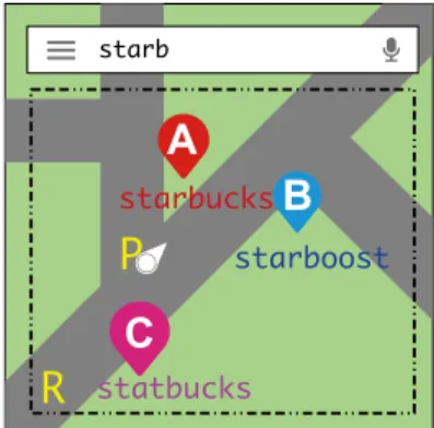
Query autocompletion is an important feature in search en- gines, command shells, desktop search, software develop- ment environments, and mobile applications. It reduces the number of keystrokes input by the users and helps improve the throughput of the system as query or intermediate results can be effectively cached and reused. With the growing popularity of mobile devices, a recent trend is to integrate query autocompletion into location-based services. One of the main applications is to complete the queries with the textual descriptions of nearby points of interest in a Web mapping service as illustrated in Example 1.

Example 1: In Fig. 1, a user at point P wants to search for nearby Starbucks. He zooms in the region around and types in the first few characters such as “starb”, and then the system automatically suggests “starbucks” and “starboost”.

The two results are also marked as points on the map asA andB.

We call this problem location-aware query autocom- pletion. A query of this problem includes a location, such as the pointPor the areaRin Fig. 1. The query also includes a string prefix, a point of interest will be returned if it is close

Manuscript received May 10, 2017.

Manuscript revised September 3, 2017.

Manuscript publicized October 5, 2017.

†The author is with Graduate School of Informatics, Nagoya University, Nagoya-shi, 464–8601 Japan.

††The author is with Institute for Advanced Research, Nagoya University, Nagoya-shi, 464–8601 Japan.

†††The author is with Graduate School of Informatics, Nagoya University, Nagoya-shi, 464–8601 Japan.

a) E-mail: [email protected] b) E-mail: [email protected] c) E-mail: [email protected]

DOI: 10.1587/transinf.2017EDP7152

Fig. 1 Location-aware error-tolerant autocompletion.

to the spatial location and its textual contents begin with the given string prefix.

In addition, the error-tolerant autocompletion also becomes very popular, because misspellings may occur due to typos in the queries or data uploaded by users, especially when users are typing with the error-prone keyboards of mobile devices. Error-tolerant feature can help to suggest correct results even when there are typos on both query prefix and data sides as showed in Example 2.

Example 2: In Fig. 1, suppose the user types in characters such as “sdarb”, and then the system with error-tolerant feature suggests “starbucks”, “starboost” and “statbucks”. The three results are marked as points on the map asA,BandC.

There have been several solutions to location-aware query autocompletion. All of them are based on a combination of spatial and textual indexes to process queries. They can be categorized into text-first[1], space-first[2],[3], and tightly-combined[4] methods, according to the ways in which the indexes are combined. For text-first methods, string descriptions of data objects are indexed in a trie, where objects as well as their locations can be retrieved on leaf nodes of the trie. For space-first methods, data objects are indexed in an R-tree or quadtree by their locations, and textual filters are applied when processing queries. For tightly-combined methods, textual and spatial information are both considered to build the index. However, all of the existing approaches suffer from inefficiency when the dataset is large, and the performance is deteriorated when large amount of simultaneous queries occur.

In this paper, we investigate the problem of location- aware query autocompletion and aim at answering range and top-k queries. We discuss the advantages of text-first Copyright c2018 The Institute of Electronics, Information and Communication Engineers

(2)

indexes over space-first and tightly-combined indexes, and propose a novel trie-based text-first method to efficiently process the two types of queries. The existing text-first ap- proachMT [1]is only applicable to top-kqueries and computes score upper bounds by enumerating query locations.

Hence the space overhead is huge, and it has to materialize score upper bounds for regions with coarse granularity and only a subset of trie nodes. UnlikeMTwhich stores on trie nodes the spatial information of queries, we choose to store the spatial information of data objects instead. Sev- eral pruning techniques are developed on top of our index.

We propose to use pointers to quickly locate data objects, in contrast toMTwhich traverses subtrees to find data objects.

In addition, the error-tolerant feature is also taken into con- sideration. We extend our method to handle this feature and suggest correct queries. Finally, we demonstrate the superiority of our solution through extensive experimental evalua- tions on real datasets.

Our contributions can be summarized as follows:

• We propose a novel location-aware query autocompletion method to efficiently answer range and top-kqueries with an acceptable index size. We are able to index a dataset with 13 million points of interest in 32GB main memory on a commodity machine, and answer both range queries and top-kqueries in microseconds or even faster.

• We integrate the error-tolerant feature into our method so as to handle the case when users input queries with error- prone devices.

• We conduct experiments to evaluate the efficiency of the proposed methods with comparisons to existing solutions.

The rest of this paper is organized as follows. Section 2 defines the problems. Section 3 surveys related work. Sec- tion 4 presents our index structure for location-aware query autocompletion. Section 5 introduces the query processing algorithms. Section 6 reports experiment results and analysis. Section 7 concludes this paper.

2. Preliminaries

2.1 Problem Definition

LetO be a set of data objects in a spatial database. Each objecto∈Ois represented by a tuple{o.str,o.loc,o.scr}. o.str is the string description. o.loc= (x,y)and describes the location in 2-dimensional space.o.scris the static score which can be used to reflect the popularity of the object.

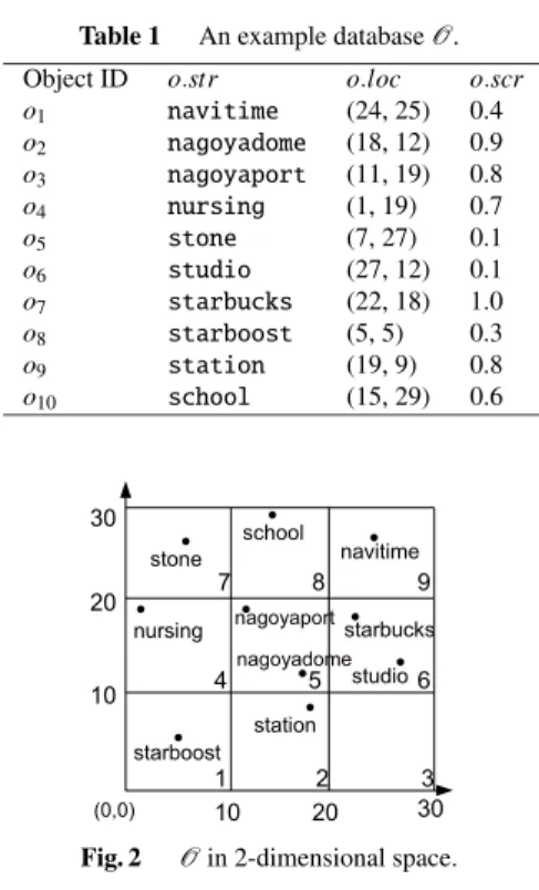
global max scrdenotes the maximum static score of the objects. global max dist denotes the maximum distance between two objects inO. An example is shown in Table 1 and Fig. 2.

Given two stringssands, “ss” denotes thatsis a prefix ofs; i.e., s=s[1..|s|]. In this paper, we focus on supporting two types of queries:

Range Query. The queryqconsists of a query stringq.str which the user is typing in and a rangeq.rngdefined by a rectangle. The answer to the queryqconsists of the objects o∈Osuch thatq.stro.strando.locis in the rangeq.rng.

Table 1 An example databaseO. Object ID o.str o.loc o.scr o1 navitime (24, 25) 0.4 o2 nagoyadome (18, 12) 0.9 o3 nagoyaport (11, 19) 0.8 o4 nursing (1, 19) 0.7

o5 stone (7, 27) 0.1

o6 studio (27, 12) 0.1 o7 starbucks (22, 18) 1.0 o8 starboost (5, 5) 0.3 o9 station (19, 9) 0.8 o10 school (15, 29) 0.6

Fig. 2 Oin 2-dimensional space.

Top-kQuery. The queryqconsists of a query stringq.str which the user is typing in and a locationq.loc. The answer to the queryqconsists of the top-kobjectso∈O such that q.stro.str, sorted by a ranking functionF(o,q). We focus on the following ranking function that gives an overall score of an object with respect to the queryq, but our method can be extended to support other monotonic functions.

F(o,q) =α· o.scr global max scr + (1−α)·

1−dist(o.loc,q.loc) global max dist

. (1)

The first component global max scr^o.scr in the ranking function measures the popularity with the object’s static score normalized into the range of [0, 1]. The second component (1−dist(o.loc,q.loc)

global max dist)measures the spatial proximity by sub- tracting from 1 the normalized Euclidean distance between the object and the query. The two components are balanced by a weight variableα. It is determined by application. A higherαindicates that the user is more towards popularity.

Whenα=0, the user only cares about proximity, and hence the query becomesknearest neighbors. When α=1, the user only cares about popularity, and hence the results are the top-kobjects ranked by static score.

Example 3: Figure 3 shows an example of a range query.

The query range is defined by the red rectangle. Suppose the query string is “sta”. The results areo7ando9. Figure 4 shows an example of a top-kquery. The query location is shown by the red cross. Suppose the query string is “na”, k=2, andα=0. The results areo2ando3.

In some applications, especially for mobile devices, the user’s input tends to contain typographical errors. In

(3)

Fig. 3 A range query.

Fig. 4 A top-kquery.

this case, we also support the error-tolerant feature so that a number of errors are allowed in the query. We choose to use edit distance to measure the input errors.ed(s,t)returns the edit distance between two stringssandt, which measures the minimum number of edit operations, including insertion, deletion, and substitution of a character, to transformstot, or vice versa. Given a thresholdτ, we return the results such that∃o.stro.str,ed(o.str,q.str)≤τ; i.e., the edit distance between the query string and a prefix of the object string is withinτ^.

In this paper, we compute the results incrementally as the user types in characters. In addition, we focus on the in- memory and stand-alone implementation of the algorithms.

3. Related Work

Location-aware Query Autocompletion. There have been several existing studies to support location-aware query autocompletion. These methods combine spatial and textual indexes. They can be divided into three categories according to the way the two indexes are combined: text- first, space-first, and tightly-combined.

Materialized Trie (MT) is a text-first method proposed by Roy and Chakrabarti[1]to find top-kresults ranked by a linear combination of static score and physical distance.

The strings of data objects are indexed in a trie, where objects as well as their locations can be retrieved on leaf nodes.

Spatial information is stored on trie nodes to speed up query processing. For each node, it divides the whole space into a grid, and stores for each region the score upper bound if the query location is in the region. MT suffers from the consumption of large amount of memory. Although a remedy was proposed to materialize a subset ofM trie nodes and

storeRbounds in each of them, it is at the expense of runtime performance.

Filtering-Effective Hybrid Indexing (FEH) is a space- first method proposed by Ji et al. [2] to answer range queries andkNN queries. The method builds an R-tree to index data objects by their locations. Textual filters are used in each R-tree node to check whether the query string is a prefix of the objects in the subtree.INSPIRE [3]is a space-first method developed for a variety of spatial-textual queries.

Data objects are indexed in a quadtree and the nodes are encoded by Hilbert curve. When traversing the quadtree, textual filtering is carried out with the help of an inverted index on theq-grams of object strings. The inverted index is partitioned as per the Hilbert curve for fast lookup. The major drawback of the space-first methods is that when the query string is short or frequent, the pruning power of the textual filters becomes very poor and thus the runtime overhead drastically increases.

Prefix Region Tree (PR-Tree)[4]is a tightly-combined method that considers textual and spatial partitioning simul- taneously to build the index. Data objects are indexed in a trie, and then each node is divided into four nodes, each representing a region in a quadtree, with centroids selected as the center for partitioning. The major problem ofPR-Tree is that although spatial conditions can be checked with the quadtree, more nodes have to be accessed for query processing due to the division of trie nodes.

Error-tolerant Query Autocompletion. Query auto- completions with edit distance to tolerate errors were first studied in[5]and[6]. Liet al. [7]improved the method proposed in[5]for space and runtime performance. More efficient methods were proposed in[8]and[9]. Apart from edit distance, cosine similarity[10]and Markov n-gram transfor- mation model[11]are also adopted for error tolerance in the autocompletion task.

Spatial Keyword Search. Given a database of points of interest (POIs) and a query composed of keywords and a location, the spatial keyword search problem is to return the relevant POIs considering both spatial proximity and textual relevance. This problem has been extensively studied in the database community. Existing solutions are based on R- tree[12]–[16], grid[17],[18], and space filling curve[19].

We also refer users to an experimental evaluation[20]that compares these methods.

4. Index Structure

In this section, we introduce our indexing method for location-aware query autocompletion.

Our index belongs to the text-first category. The rea- sons why we resort to a text-first index are:

• For location-aware query autocompletion, a common sce- nario is that the query string is short, hence rendering the text filter of space-first indexes unselective. E.g., the fre- quency of the q-gram “an” is 0.18 in the FSQ dataset, which consists of 1 million worldwide points of inter-

(4)

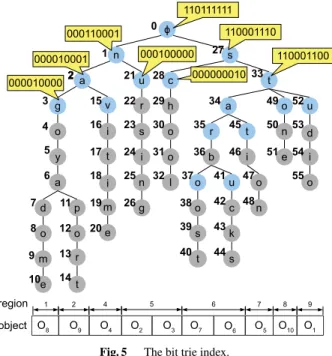
Fig. 5 The bit trie index.

est collected from Foursquare, meaning that on average at least 18% objects under a tree node will be fetched for verification if the query string contains a character pair “an”. In contrast, text-first indexes are based on a trie. We only need to traverse the trie to match the query string, and thus good query processing performance can be achieved.

• Tightly-combined indexes exhaustively divide nodes in the tree using spatial information, thus resulting in redundant node access when processing queries. For text- first indexes, because a trie is compact (given a query string, there is only one matching path), node access can be saved.

• To verify spatial information in text-first indexes, we may equip trie nodes with spatial filters and verify spatial conditions efficiently when fetching data objects under a trie node.

• It is easy to implement and flexible to choose data structures for spatial access, e.g., R-tree, quadtree, grids, etc.

Note that a brief explanation of choosing text-first index also appears in[1], which also adopts the text-first method, but from different perspectives: (1) text-first method is able to support any ranking function, and (2) text-first method is optimum in space requirement.

The basic structure of our index is a trie built on the set of object strings. Each node is uniquely identified by a string corresponding to the labeled path from the root to the node, so that search can be easily performed by identifying the node that matches the query string. Given a node in the trie, we say a data object is anunderlying objectof this node if the path from the root to the node is a prefix of the object string. If we run a pre-order traversal in the trie, each node can be assigned a number by the order in which they are accessed. Consider the objects in Table 1. Figure 5 shows the trie in which the object strings are indexed. Nodes are

numbered by the pre-order traversal. o1 is an underlying object of node 2, becausenais a prefix ofnavitime.

Next we introduce how to integrate spatial data structure into the trie. First, the global space is partitioned into a set of spatial regions. This step can be done using common data structures for spatial objects, such as grid, R-tree, quadtree, etc. The partitions can be either overlapping (e.g., by an R-tree) or non-overlapping (by a grid). A region represents a cell if we use a grid to partition the space, and a leaf node if we use a tree-based data structure. For ease of illustration, we describe our method by assuming the space is partitioned by a grid, although experimental evaluation shows that partitioning by a quadtree yields better query processing performance.

Each object belongs to a region with respect to the spatial partitioning. We equip each node in the trie with a bit array, each bit representing a region. A bit is set to 1 if the node has an underlying object in this region; or 0, otherwise. We call itregion bit array. With this bit array, when searching in the trie, we are able to check whether there is an underlying object in the region that intersects the query range.

Example 4: Assume that the space is partitioned as per the grid in Fig. 2. We show in Fig. 5 the region bit arrays of the nodes in the first three levels. Then-th bit represents the cell numberednin Fig. 2.

We observe that some nodes share the same region bit arrays as their parents in the trie. In this case, the child nodes’ bit arrays are redundant and have no pruning power for query processing, and hence we only keep the bit array of the parents to save space and search time. We also use a flag SameAsParenton these child nodes so that when we need to retrieve their bit arrays, their parents are referred to.

For example, in Fig. 5, all the nodes under 3 have the same bit array 000010000 as node 3. We only keep the bit array 000010000 at the node 3, and remove those at its descendant nodes. In Fig. 5, a node is colored grey if it shares the same bit array as its parent.

Data objects are stored in an array called data ob- ject array, which is partitioned into spatial regions as well.

Since an object string corresponds to a leaf node in the trie, within each region in the data object array, we sort objects in the order of their corresponding leaf nodes in the trie. To quickly identify underlying objects in the array, each node in the trie is equipped with a list calledregion list, whose entries are in the form ofregion ID,maximum static score, starting pointer,ending pointer . The maximum static score of an entry is the maximum static score of the node’s underlying objects in this region, and it is used to efficiently answer top-kqueries. The starting and ending pointers are used to fetch results in the data object array. They are linked to the starting and ending positions in the partial array that contains the underlying objects of the node in this region, respectively. Entries in the list are sorted by descending maximum static score order.

(5)

Example 5: Consider node 2 in Fig. 5. Its region list is [5,0.9,4,5 ,9,0.4,10,10 ]. The maximum static score of this node is 0.9.

For index construction, one may notice that if siblings in the trie are arranged in alphabetical order, the objects in each region in the data object array follow the lexicographical order. This property facilitates the index construction:

Given the set of data objectsO, we divide it with the partitioning first, and then sort the objects in each region by lexicographical order. The trie is initialized as empty. For each region, the objects are scanned one by one, and their strings are inserted into the trie. Once a string is inserted, we update the region bit arrays and the region lists of the nodes on the path, as well as the maximum static scores of the nodes. The time complexity of the index construction is O(OlogO+S), whereS is the sum of string lengths of the objects.

5. Query Processing Algorithms

The query processing algorithms are introduced in this section. We first present the algorithms for answering range queries and top-kqueries, respectively, and then show how to extend them to cope with the error-tolerant case.

5.1 Processing Range Queries

The query processing is divided into two phases: (1) searching phase, in which the query string is looked up in the trie and the spatial condition is checked; and (2) result fetching phase, in which the data object array is accessed to fetch and return results.

We begin with the searching phase. To process a query q.str,q.rng , we first compareq.rngwith the spatial partitioning and obtain the regions occupied byq.rng. We ini- tialize a bit array, where a bit is set to 1 ifq.rngintersects a region; or 0, otherwise. The bit array is calledregion status.

For example, the initial region status for the query in Fig. 3 is 011011000 because the query range intersects regions 2, 3, 5, and 6 in the grid.

Then we start to traverse the trie with the query string.

As the user types in the query, we follow the path that matches the query string. For each node, the region status is updated by a bitwiseANDoperation with the region bit array of the node. Since the region bit array keeps track of whether there is an underlying object in a region, if a bit becomes 0 after the bitwiseANDoperation, it means that there is no underlying object in this region for the query. We say a node is anactive nodeif its path matches the query string and the region status is not all zero. The traversal in the trie is essentially to check if there is an active node for the next keystroke input by the user. Whenever there is no path matching the query string or the region status becomes all zero, we can stop the traversal of the trie and return no results.

The above process is shown in Algorithm 1. It takes

as input the query and the trie. First, a region status is initialized (Line 1). Then it traverses the trie to match the next keystroke (Line 4) and update the region status (Line 5). If this is no match for the keystroke or the region status becomes all zero, it exits the traversal. It returns the active node and the region status for result fetching, or null to in- dicate there is no result (Line 14). The time complexity is O(|q.str|), where||denotes the length of a string.

We also observe that if a bit in the region status becomes 0 during the traversal, it will never return 1. Hence a blocking technique can be devised to save bitwise operations. We divide region bit arrays and the region status into equi-width blocks (e.g., 64-bit blocks), and only keep the blocks with at least a 1 in the region status.

The result fetching phase of range query is as follows.

We obtain the bits equal to 1 in the region status, and scan the corresponding regions in the region list. With the starting and ending pointers, the objects in the data object array are located. Each object between the two pointers is verified with the query for the spatial constraint; i.e., if the location of the object is within the query range. The object is returned as a result if it passes this verification. The pseudocode of the result fetching phase is shown in Algo- rithm 2, which reads in the active node n and the region statusb, and returns the result setR. The time complexity isO(Σ^|_i=1^L^|ei−si+1), whereLdenotes the region list,siand eidenote the starting and ending pointers of thei-th entry in the list, respectively.

(6)

Example 6: Consider the query range in Fig. 3 and a query strings. The region status is initialized as 011011000. We start with the root and traverse the trie. Since there is an edge s, we follow this edge and reach node 27. Its region bit array is 110001110. By bitwiseAND operation, the region status becomes 010001000. The node’s region list is[1,0.3,1,1 ,2,0.8,2,2 ,6,1.0,6,7 ,7,0.1,8,8 , 8,0.6,9,9 ]. With the region status, regions 2 and 6 in the list are accessed. For region 2, the pointers are 2 and 2.

So we scan the 2nd objecto9in the data object array, and verifies it as a result. For region 6, the pointers are 6 and 7. So we scan the 6th and 7th objects in the array. o7is in the query range and becomes a result, whileo6fails the verification. The final results areo7ando9.

5.2 Processing Top-kQueries 5.2.1 Basic Algorithm

The algorithm framework of processing top-kqueries is similar to processing range queries, except that the region status is not involved as there is no spatial constraint. The pseudocode of the searching phase is given in Algorithm 3. It matches the input keystrokes and follows the path in the trie to find the active node.

Algorithm 4 captures the basic result fetching algorithm for top-kqueries. It initializes a priority queue of size kto store temporary results (Line 2). Then it iterates through the region list of the active node (Line 3), retrieves objects in the data object array (Line 4), and computes the overall score by Eq. (1) (Line 5). If the priority queue has less than kresults or the score is greater than thek-th temporary result, we insert into the queue the object accompanied with its score. The queue containing the top-kresults is returned

eventually as the final results (Line 8). The time complexity isO(Σ^|L|_i₌₁ei−si+1), whereLdenotes the region list,siand eidenote the ending and starting pointers of thei-th entry in the list, respectively.

The basic result fetching has to scan all the entries in the active node’s region list and all the objects bounded by the pointers. If we scan less number of elements in the two processes, the query processing performance can be improved. Next we present two major optimizations for the purpose of early termination.

5.2.2 Region Level Pruning

The first optimization is to scan only part of entries in the region list. Recall that the entries in the list are sorted by descending order of maximum static score. Given the score of thek-th temporary result and the maximum static score of the i-th entry in the list L, a distance threshold can be computed:

dt=global max dist·

⎛

⎝1− ·R[k].scr−α·global max scr^L[i].m

1−α

⎞

⎠. (2) R[k].scrandL[i].mrepresents the score of thek-th temporary result and the maximum static score of thei-th entry in the listL, respectively. Then, a distance thresholddt can be computed from Eq. (1). It means that if any unseen object is better than thek-th temporary result, its distance to the query must be smaller than the distance threshold dt. With the location of the query, we can compute the regions that are close enough to the query to meet this condition, and record these regions in a bit array. A bit is set to 1 if the distance from the region to the query is less thandt; or 0, otherwise. We may invoke a bitwiseANDoperation between this bit array and the active node’s region bit array. If the result is all zero, all the regions are beyond the distance threshold, and hence all the entries in the region list can be pruned.

With the above property, a pruning algorithm is developed. Its pseudocode is given in Algorithm 5, and we use it to replace Lines 3 – 7 of Algorithm 4. A bit arraybis initialized as the active node’s region bit array (Line 1). When processing each regionrin the region list, the distance threshold is computed first (Line 6) by Eq. (2). With the threshold, we generate the bounded regions (Line 7) that are close enough to the query. The regions are represented by a bit arrayb. We take a bitwiseANDoperation betweenband b, and write the result tob(Line 8). Ifbbecomes all zero, it is guaranteed that no regions in the remaining list contain an object better than thek-th temporary result, and thus we stop scanning the region list (Line 10). Otherwise, (1) if the bit that representsrinbis zero,ris skipped; (2) otherwise, we fetch results inrand update the temporary results (Lines 13 – 16). Because this pruning technique is applied on the region level, we name itregion level pruning.

(7)

Table 2 Bounded regions with varying distance thresholds.

Distance Threshold Bit Array

t=0 000000000

0<t≤0.082 001000000 0.082<t≤0.164 011000000 0.164<t≤0.183 011001000 0.183<t≤0.318 011011000 0.318<t≤0.358 111011000 0.358<t≤0.400 111111000 0.400<t≤0.408 111111001 0.408<t≤0.511 111111011 t≥0.511 111111111

Example 7: Consider the objects in Table 1. The query string is na. Its location is shown in Fig. 4. k=2, and α=0.5. Supposeglobal max dist=1. The distances from the query too2, o3, and region 9 are 0.3, 0.5, and 0.4, respectively.

We follow the pathna, the active node is node 2 in the trie. Its region bit array is 000010001, and its region list is[5,0.9,4,5 ,9,0.4,10,10 ]. We first process region 5.

After that, the top-ktemporary results as well as their scores areo2,0.8 ando3,0.65 . The bit arraybis 000010001.

Next we process region 9. By Eq. (2), the distance threshold is 0.1. The bounded regions are 2 and 3. Sobis 011000000.

A bitwiseANDoperation onbandbyields all zero. So we can prune region 9 and returno2ando3as the final results.

There are two minor optimizations on the region level pruning. First, since the bounded regions only depend on the query location and the distance threshold, we can pre- compute all the possible bounded regions once the query location is received. We do not have to enumerate all the distance thresholds but only consider the values at which the bounded regions change. For example, for the query whose location is shown in Fig. 4, Table 2 lists the bit arrays for the bounded regions under different distance thresholds.

Second, due to the bitwiseANDoperation, a bit inbnever returns 1 if it becomes 0. So we may use the blocking tech-

nique to dividebinto equi-width blocks, and only keep those with at least a 1 to save bitwise operations.

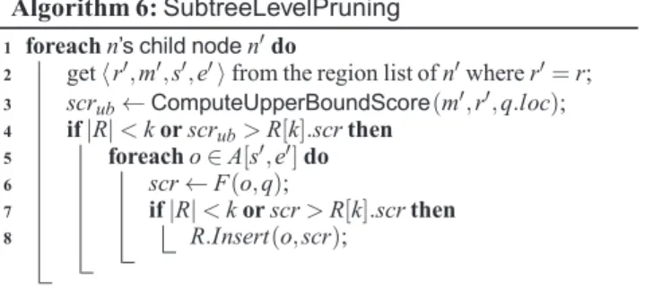
5.2.3 Subtree Level Pruning

The second optimization is to reduce the number of objects to access in the data object array. Recall that in the basic result fetching algorithm we directly go through the objects between the two pointers. On the other hand, it can be observed that for a nodenand a regionr, if we fetch objects of rfrom alln’s children, they exactly constitute the underlying objects ofninr. Since the maximum static scores have been recorded in the region lists of the child nodes, we may compute a score upper bound from Eq. (1):

scrub=α· m global max scr + (1−α)·

1− dist(r,q.loc) global max dist

, (3)

wheremdenotes the maximum static score of regionrinn’s child node, anddist(r,q.loc)denotes the distance between region rand the query location. If the upper bound is no better than thek-th temporary result, we can skip all the objects between the starting and ending pointers of the child node in this region; i.e., all the objects specified by the subtree rooted as this child node. We leverage this property and devise a pruning algorithm (calledsubtree level pruning) as follows.

Algorithm 6 provides the pseudocode of the subtree level pruning. It replaces Lines 13 – 16 in Algorithm 5.

Consider we are fetching objects in regionrfor noden. In- stead of directly fetching from node n, we iterate through all its child nodes (denoted byn). The entry with region ID equals torin the region list ofnis identified (Line 2).

We retrieve the corresponding maximum static scorem, and compute a score upper bound (Line 3). If the upper bound is no greater than the score of thek-th temporary result, we skip noden. Otherwise, we access the data object array and fetch the objects between the corresponding pointerssand eto update the temporary results (Lines 5 – 8).

Example 8: Consider the objects in Table 1. The query string isnagoya. Its location is shown in Fig. 4. Suppose thatk=1, andα=0.5. Supposeglobal max dist=1. The distances from the query too2ando3are 0.3, 0.5, respectively.

(8)

We follow the pathnagoya, the active node is node 6 in the trie. There is only region 5 in the node’s region list. By subtree level pruning, we first process the first child – node 7 and find one temporary resulto2, whose score is 0.8. Then we process the second child – node 11. By Eq. (3), the score upper bound is 0.65. It is smaller than thek-th temporary result’s score. So node 11 is pruned, and we returno2as the final result.

To apply subtree level pruning, one subtlety is to find the entry with region ID equals torfrom the region list ofn. We first test the corresponding bit in the region bit array of n. If the bit is 0,nis skipped, meaning there is no regionr in the region list. Otherwise, we scan its region list until the region IDrappears. The following optimization is applied while we scan the region list. Since the list has been sorted by descending order of maximum static score, for eachm we see in the list, no matter which region it corresponds to, we may compute a score upper bound by Eq. (3) as if m was the maximum static score of regionr. If the upper bound is no greater than thek-th temporary result’s score, we can stop the scan and skip noden even if we have not seen regionryet.

One may notice that subtree level pruning can be carried out recursively; i.e., to go deeper in the trie and prune more objects using the region lists of noden’s grand descen- dants. We choose not to do so because probing the region lists poses overhead, and our experiments show that con- ducting subtree level pruning only onn’s children achieves a balance between pruning objects and list entry access.

5.3 Supporting Error-Tolerant Features

Our method can be easily integrated into the existing solutions to error-tolerant query autocompletion; such as[5], [6],[8],[9]. We choose the trie-based method proposed in [6]for ease of illustration.

The basic idea of the method in [6] is to process the keystrokes in the query and compute a set of active nodes in the trie. The trie is exactly the same as ours except that we store spatial information on it. The path from the root to an active node is a string whose edit distance to the query is within the thresholdτ. For example, supposeτ=1. Given a query string “ni” and the trie in Fig. 5, nodes 1, 2, and 21 are active nodes, becausen,na, andnuare the strings whose edit distances toniare 1. Therefore, we need to extend our method from single active node to the multiple active node case.

For range queries, we replace Line 4 in Algorithm 1 with the active node propagating method in[6]. In Algo- rithm 4, we change its input by replacingn with a set of active nodes, and fetch result for every active node inside the algorithm.

For top-kqueries, we do the same replacement in Al- gorithms 3 and 4. In addition, an optimization technique is applied for faster result fetching. Since the region list of a node is sorted by descending maximum static score order,

the first entry gives the maximum static score among all the underlying objects of the node. We choose to sort the nodes by the descending order of this value, and then process them one by one using Algorithm 4. For an active node n, we can compute an upper bound of its underlying objects from Eq. (1):

scrub=α· max scr(n)

global max scr+1−α, (4) wheremax scr(n)denotes the maximum static score among the underlying objects ofn. The upper bound is compared with thek-th temporary result. If it is no greater than thek-th temporary result’s score, we can terminate the result fetching phase and output final results, because the remaining active nodes cannot produce any underlying object better than the current top-kobjects. We call this optimizationactive node level pruning.

Before reporting experiment results, we briefly discuss the differences between our method and theMTmethod[1]:

• Although both methods use trie-based text-first indexes, we use region bit array for pruning to speed up query processing, while there is no such data structure or pruning technique inMT.

• In the indexing step, MTenumerates the query location across all the regions and stores the corresponding score upper bounds in the trie nodes. This drastically increases memory consumption, and thusMThas to materialize the score upper bounds for regions with coarser granularity and only a subset of trie nodes. Although this technique makes MTmeet the space requirement, it compromises query processing performance. In contrast, our method materializes region lists without any compromise because the regions under most trie nodes are sparse (see Exam- ple 5).

• For query processing, we use pointers to locate the objects in the data object array to fetch results, while MT traverses the subtree rooted at the active node.

6. Experiments

We report the experiment results in this section.

6.1 Experiment Setup

The following algorithms are compared in the experiment.

• Tregion is our proposed method. It is based on atrie integrated withregioninformation. Space is partitioned by a quadtree, and each leaf node is regarded as a region.

• MT is a trie-based text-first method for top-kqueries[1].

• PR-Tree is a tightly-combined method that merges trie and quadtree into a single index[4]. It was designed for processingknn queries.

• INSPIRE is a quadtree-based space-first method[3].

It was proposed for the spatial-textual query relaxation problem. It answers range queries in an error-tolerant manner.

(9)

Fig. 6 Performance on range queries.

Table 3 Dataset statistics.

Dataset |O| size avg. string length

FSQ 1,021,447 31 MB 9.4

GNIS 2,193,355 67 MB 10.9

SGP 12,705,409 394 MB 11.5

For our method, we adjust the capacity in the quadtree node, and the number of resulting regions is no more than 64, which gives best query processing performance. We use the method proposed in[6]to process error-tolerant queries. For the other competitors, we make minor modifications so they can answer both range queries and top-kqueries as well as error-tolerant queries. ForMT, we use the same region set- ting as forTregion, and materialize score upper bounds for all trie nodes. We do not compare with theFEHmethod[2]

as it has been shown to be significantly outperformed by PR-TreeandINSPIRE [3],[4].

We select three publicly available datasets:

• FSQis a dataset collected from Foursquare, which contains 1M worldwide points of interest.

• GNIS is a dataset of 2M geographic names collected from the U.S. Government Geographic Names Informa- tion System.

• SGPis a dataset of 13M records obtained from Simple- Geo’s Places.

Table 3 shows statistics about the datasets.

For each type of query, we generate 1,000 random queries by choosing strings that appear in the dataset. Lon- gitude and latitude are normalized to [0, 1]. The default query range is a 0.08×0.08 square. The default value ofk is 10.

We measure (1) average query response time, including both searching time and result fetching time, (2) index construction time, and (3) index size.

The experiments were carried out on a PC with an In- tel i5 2.6GHz Processor and 32GB RAM, running Ubuntu 14.04.3. The algorithms were implemented in C++ and in a main memory fashion.

6.2 Range Queries

The performance of processing range queries is evaluated first. Figure 6 (a) – 6 (c) show the query processing times of the four algorithms on the three datasets, varying query string length. Because the number of results decreases when the query becomes longer, the general trend is that the query

processing times decrease with the query string length, thoughPR-TreeandINSPIREshow some rebounds due to more traversal cost when the query is longer than 5 characters. Thanks to the region bit array,Tregionis always faster than the other competitors. The speedup can be up to one to two orders of magnitude.PR-Treeis the second fasters, and the INSPIREis the third. We observe that the number of node access ofPR-Treeis significantly higher thanTregion.

E.g., on FSQ dataset, when the query string length is 4, the average numbers of node access of PR-Tree andTregion are 154.3 and 3.3, respectively. The reason whyINSPIREis slow is that most query processing time is spent (e.g., 87.9%

on the SGP dataset when the query string length is 2) on the text filter based onq-grams, whose frequencies are high for short strings (e.g., “an”) and thus not selective. These results show the drawbacks of the tightly-combined method and the space-first method, hence justifying our analysis on the three types of methods in the beginning of Sect. 4. MT is the slowest in most cases, because it does not have any spatial filter in the searching phase and the spatial condition is checked when we fetch results.

6.3 Top-kQueries

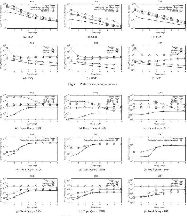
For top-kqueries, we first evaluate the effects of the pruning techniques. Figure 7 (a) – 7 (c) show the result fetching times on the three datasets for the four algorithms:Tregion, Tregion with region level pruning only, Tregionwith subtree level pruning only, andTregionwithout the two pruning techniques. It can be observed that both pruning techniques effectively decrease the query processing time ofTregionby 2 to 28 times, and they are more effective for short queries.

The comparison with the other methods on the three datasets are shown in Fig. 7 (d) – 7 (f). Due to the algorithm design for top-kqueries and the effects of two pruning techniques, Tregionis the fastest of the four algorithms, and it is up to 4 times faster than the runner-upMT.PR-Treeis the third and INSPIREis the slowest method. Both are slower thanTre- gionby one to two orders of magnitude. The drawbacks of the tightly-combined method and the space-first method are also seen on top-kqueries. E.g., on FSQ dataset, when the query string length is 4,PR-Treeaccesses 289.3 nodes on average whileTregionaccesses 14.2 nodes. ForINSPIRE, when query string length is 2 on the SGP dataset, 90.5%

query processing time is spent on the text filter, and thus the query processing speed becomes slow.

(10)

Fig. 7 Performance on top-kqueries.

Fig. 8 Performance with error-tolerant feature.

6.4 Error-Tolerant Queries

We enable the error-tolerant feature and show the query processing times of range queries in Figs. 8 (a) – 8 (c). The edit distance threshold is 3. The query processing time ofTre- gionincreases when more characters are input. The reason is that we have more traversal in the trie to tolerate errors,

and it increases the overall cost when the query becomes longer. Nonetheless,Tregion is the fastest among the four algorithms, and the speedup can be up to two orders of magnitude.

For error-tolerant top-kqueries, we first evaluate the effect of active node level pruning and show the results in Figs. 8 (d) – 8 (f). The active node level pruning is more effective for short queries, because there are more active nodes

(11)

Fig. 9 Performance when varying dataset size.

Fig. 10 Performance when varying range ork.

for the first few characters and hence more chance to prune.

The comparison with the competitors on error-tolerant top-k queries is shown in Figs. 8 (g) – 8 (i). Tregionis the fastest algorithm, and the runner-up isMT. Both are faster thanPR- TreeandINSPIREby a remarkable margin (up to 9 times).

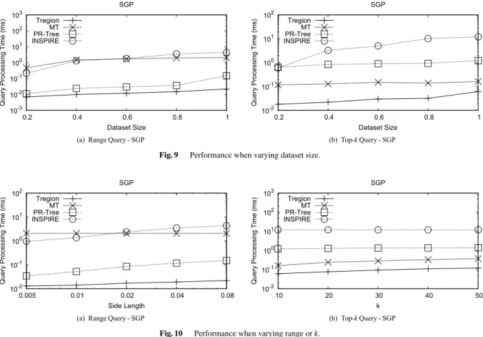
6.5 Scalability

We evaluate the scalability of the algorithms with varying dataset size. Figures 9 (a) and 9 (b) show the range query and top-kquery performances on the SGP dataset, respectively. The query processing times increase with the dataset size for the four algorithms. Tregionis always the fastest, and it has slower growth rate than the other three competitors.

We also test the performances of the four algorithms when varying range for range queries orkfor top-kqueries.

Figure 10 (a) shows the query processing times for the following range queries: 0.005×0.005, 0.01×0.01, 0.02× 0.02, 0.04×0.04, and 0.08×0.08. MT’s query processing time is regardless of the query range because it does not have any spatial filter for range queries. The other three algorithms exhibit increasing query processing time when the query range expands. This is expected as there are more tree nodes satisfying the spatial condition and the number of results also increases. Figure 10 (b) shows the query processing times for the followingkvalues: 10, 20, 30, 40, and 50.

Table 4 Index size (GB).

Dataset Tregion MT PR-Tree INSPIRE

FSQ 1.4 8.6 0.5 0.5

GNIS 1.6 8.9 1.0 0.9

SGP 13.4 32.0 5.3 6.3

Table 5 Index construction time (seconds).

Dataset Tregion MT PR-Tree INSPIRE

FSQ 11.3 81.4 4.7 12.7

GNIS 17.5 141.1 9.0 23.2

SGP 178.5 958.1 54.4 190.6

INSPIREhas almost constant query processing time when kvaries because it was designed for range queries, lacking specific filters for top-kqueries. For the other three algorithms, the running times slightly increase when kmoves towards larger values. Tregionis always the fastest among the four competitors.

6.6 Index Construction

Table 4 shows the index sizes of the four algorithms on the three datasets. Table 5 shows the corresponding index construction times.MThas the largest index size due to its enu- meration of query locations.Tregion’s index size is the second among the four, but is much smaller thanMT.PR-Tree andINSPIREhave similar index sizes. All of the four algo-

(12)

rithms are able to build index in reasonable amount of time.

MTis the slowest of the four.Tregionspends less time than INSPIREbut more time thanPR-Tree.

7. Conclusion

In this paper, we proposed a novel method for location- aware query autocompletion. We aimed at answering range and top-kqueries on a large scale. We proposed a method by which data objects are indexed in a trie integrated spatial information. Several pruning techniques were proposed to further improve the query processing performance. We also discussed how to extend our method to support the error tolerant feature. The experiment results demonstrate the efficiency of the proposed method and its superiority over existing methods.

Acknowledgements

This research was partly supported by the Grant-in-Aid for Scientific Research (16H01722) from JSPS.

References

[1] S.B. Roy and K. Chakrabarti, “Location-aware type ahead search on spatial databases: semantics and efficiency,” ACM SIGMOD 2011, pp.361–372, 2011.

[2] S. Ji and C. Li, “Location-based instant search,” Int’l Conf. Scientific and Statistical Database Management (SSDBM 2011), vol.6809, pp.17–36, 2011.

[3] Y. Zheng, Z. Bao, L. Shou, and A.K.H. Tung, “INSPIRE: A framework for incremental spatial prefix query relaxation,” IEEE TKDE, vol.27, no.7, pp.1949–1963, 2015.

[4] R. Zhong, J. Fan, G. Li, K.-L. Tan, and L. Zhou, “Location-aware instant search,” ACM CIKM 2012, pp.385–394, 2012.

[5] S. Ji, G. Li, C. Li, and J. Feng, “Efficient interactive fuzzy keyword search,” WWW 2009, pp.371–380, 2009.

[6] S. Chaudhuri and R. Kaushik, “Extending autocompletion to tolerate errors,” ACM SIGMOD 2009, pp.707–718, 2009.

[7] G. Li, S. Ji, C. Li, and J. Feng, “Efficient fuzzy full-text type-ahead search,” VLDB J., vol.20, no.4, pp.617–640, 2011.

[8] C. Xiao, J. Qin, W. Wang, Y. Ishikawa, K. Tsuda, and K. Sadakane,

“Efficient error-tolerant query autocompletion,” PVLDB, vol.6, no.6, pp.373–384, 2013.

[9] D. Deng, G. Li, H. Wen, H.V. Jagadish, and J. Feng, “META: an efficient matching-based method for error-tolerant autocompletion,”

PVLDB, vol.9, no.10, pp.828–839, 2016.

[10] Z. Bar-Yossef and N. Kraus, “Context-sensitive query autocompletion,” WWW 2011, pp.107–116, 2011.

[11] H. Duan and B.J.P. Hsu, “Online spelling correction for query completion,” WWW 2011, pp.117–126, 2011.

[12] I.D. Felipe, V. Hristidis, and N. Rishe, “Keyword search on spatial databases,” ICDE 2008, pp.656–665, 2008.

[13] A. Cary, O. Wolfson, and N. Rishe, “Efficient and scalable method for processing top-k spatial boolean queries,” Int’l. Conf. Scientific and Statistical Database Management (SSDBM 2010), vol.6187, pp.87–95, 2010.

[14] Z. Li, K.C.K. Lee, B. Zheng, W.-C. Lee, D. Lee, and X. Wang,

“Ir-tree: An efficient index for geographic document search,” IEEE TKDE, vol.23, no.4, pp.585–599, 2011.

[15] D. Wu, G. Cong, and C.S. Jensen, “A framework for efficient spatial web object retrieval,” VLDB J., vol.21, no.6, pp.797–822, 2012.

[16] D. Wu, M.L. Yiu, G. Cong, and C.S. Jensen, “Joint top-k spatial keyword query processing,” IEEE TKDE, vol.24, no.10, pp.1889–1903, 2012.

[17] S. Vaid, C.B. Jones, H. Joho, and M. Sanderson, “Spatio-textual indexing for geographical search on the web,” Int’l. Symp. Spatial and Temporal Databases (SSTD 2005), pp.218–235, 2005.

[18] A. Khodaei, C. Shahabi, and C. Li, “Hybrid indexing and seamless ranking of spatial and textual features of web documents,” DEXA 2010, vol.6261, pp.450–466, 2010.

[19] M. Christoforaki, J. He, C. Dimopoulos, A. Markowetz, and T. Suel,

“Text vs. space: efficient geo-search query processing,” ACM CIKM 2011, pp.423–432, 2011.

[20] L. Chen, G. Cong, C.S. Jensen, and D. Wu, “Spatial keyword query processing: An experimental evaluation,” PVLDB, vol.6, no.3, pp.217–228, 2013.

Sheng Hu is a Ph.D. candidate in Graduate School of Information Science, Nagoya Univer- sity. He received B.E. degree from North China Electric Power University in 2013. His research interests include textual databases and spatio- temporal databases.

Chuan Xiao is an assistant professor in Graduate School of Information Science, Nagoya University. He received B.E. degree from Northeastern University, China in 2005, and Ph.D. degree from The University of New South Wales in 2010. His research interests include data cleaning, data integration, textual databases, and graph databases. He is a member of DBSJ.

Yoshiharu Ishikawa is a professor in Graduate School of Informatics, Nagoya Uni- versity. He received B.S., M.E., and Dr. Eng.

degrees from University of Tsukuba in 1989, 1991, and 1995, respectively. His research interests include spatio-temporal databases, mobile databases, sensor databases, data mining, information retrieval, and e-science. He is a member of ACM, DBSJ, IEEE, IEICE, IPSJ, and JSAI.