Development of a Small-spin-axis Controller and Its Application to a Solar Sail Subpayload Satellite

Development of a Small-spin-axis Controller and Its Application to a

Solar Sail Subpayload Satellite

By Takanao SAIKI, Koji NAKAYA, Takayuki YAMAMOTO, Yuichi TSUDA,

Osamu MORI and Jun’ichiro KAWAGUCHI

The Institute of Space and Astronautical Science / Japan Aerospace Exploration Agency, Sagamihara, Japan

(Received January 13th, 2009)

The instruments and actuators in the attitude control system of small spacecraft are restricted in weight and space, and need to be reduced in weight and size. The rhumb line control strategy is one of the most popular schemes in reorientation of spin-stabilized spacecraft, since it requires only a spin sun sensor and a single axis reaction control system. By being combined with active nutation control, rhumb line control can reorient the spin axis of the spacecraft to any direction. To verify the control strategy, we manufactured an attitude controller and demonstration experiments were conducted using a motion table at ISAS/JAXA. This paper reviews the configuration of the controller and the outlines of the experiments, and evaluates the control performance. The same type of controller was installed in the Solar Sail Subpayload Satellite (SSSAT) launched in September 2006. An attitude control experiment in orbit was not conducted because of trouble with the satellite, but new control logic for the SSSAT was implemented for the attitude controller. This paper also reviews the control logic of the SSSAT.

Key words: Spin-axis-control, Rhumb Line Control, Active Nutation Control, Solar Sail Subpayload Satellite

1. Introduction

Recently, there has been substantial interest in compact satellite technologies. Small satellites can be developed in two years or less, and there are many more opportunities for launches by utilizing the remaining space and capabilities of the rockets. Small satellites are now indispensable for the demonstration of new space technologies. However, the size and weight of the satellite are strictly restricted. Therefore, it is very meaningful to develop simple small attitude control systems for small satellites.

Spin stabilization is the simplest means of satellite attitude control and it can be applied for many space missions, such as for lunar probes 1),2) _{and small rockets.}

A reaction jet system is required for the up/down spin control and spin axis reorientation. As the common hydrazine thruster system is heavy and complicated, it is difficult to apply to small satellites. But the gas-liquid

equilibrium thruster3) _{system developed at ISAS/JAXAis}

very useful for small satellites. The gas-liquid equilibrium thruster utilizes gas-liquid equilibrium pressure for propulsion. The pressure of the gas is small, but it becomes possible to reduce the weight of the tank and pipeline. Small spin-stabilized satellites become feasible using this gas-liquid equilibrium thruster system.

The rhumb line control is one of the most popular

schemes in the reorientation of spin-stabilized spacecraft because it requires only a spin type sun sensor. As the rhumb line control cause nutation motion, active nutation control after rhumb line control is necessary for precise spin-axis control.

In order to verify the control logic of rhumb line control and active nutation control, we manufactured a test model of the controller and demonstration experiments were conducted using a motion table at ISAS/JAXA. The motion table is a 3-dimensional attitude motion simulator, and it can realize any 3-dimensional attitude of a spacecraft. Using this motion table, it becomes possible to verify the performance of the control laws and sensors.

The control system developed was applied to the attitude controller of the Solar Sail Subpayload Satellite (SSSAT). ISAS/JAXA has been studying a solar sail mission concept for future applications to deep space exploration. One of the key technologies of the solar sail mission is how to deploy/maintain the large flexible membrane. Several kinds of solar sail deployment/ maintenance methods have been investigated. The spin-type solar sail has been studied at ISAS/JAXA, and demonstration experiments with a sounding rocket and balloon have been conducted4),5)_{. For the next step of solar}

sail research, the SSSAT was launched using the 7th M-V rocket as the subpayload in September 2006. The main goal of the SSSAT was to demonstrate sail deployment and attitude control for satellite with large membrane. The following missions were assigned;

• Electric power supply with a thin-film solar cell.

• Orbit determination with a small GPS receiver. • Demonstrate the distributed heater control system. • Measure particle density in orbit using a dust

counter.

Separation from the rocket was confirmed by pictures from the rocket telemetry, but telemetry data was not received because of trouble with the telemetry system.

In this paper, the control logic of the rhumb line control and active nutation control is described and the system configuration of the attitude controller is shown. This paper then reviews an outline of the experiment and evaluates the control performance. Finally, the new attitude control logic of the SSSAT is shown.

2. Control Logic 2.1. Rhumb line control

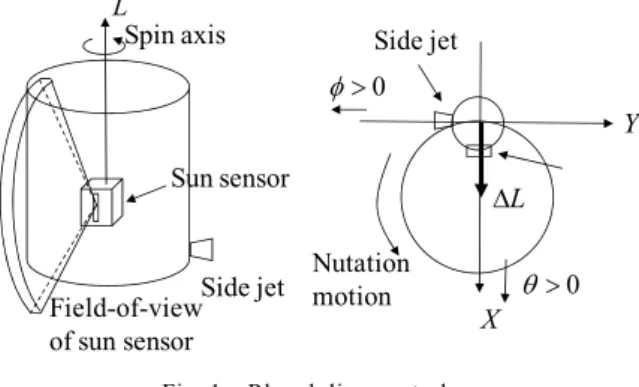
The rhumb line control is the simplest method for reorientating the direction of angular momentum of the spinning spacecraft. The spinning spacecraft depicted in Fig. 1 is considered here. This spacecraft is equipped with a spin-type sun sensor and a side jet. This sun sensor has a slit and the field-of-view is shown in the left-hand figure. It can sense the sun pulse and measure the angle between the sun direction and spin axis. Although one or more attitude sensors are necessary to determine the spin axis direction, they are omitted here.

Y X 0  0  L  Nutation motion Spin axis L Field-of-view of sun sensor Sun sensor Side jet Side jet

Fig. 1 Rhumb line control.

The side jet is equipped to give external torque. When the external pulse torque is given as the right-hand figure, the equation of motion can be written as follows:

0 ( ) 0 x y y x I J N t I J           _{  }    , (1) where , , ( ) .T x y z x y I I I J I 　ω    The solution

when xy0 can be written as follows;

0 0 0 0 / cos( / ) / cos ' / sin( / ) / sin ' x y N I J I t N I t N I J I t N I t          _{  }  . (2)

Then the attitude angles become;

0 2 2 2 0 0 0 sin ' ' ' ' (1 cos ' ) ' N t N N I N I I t I    _{ }        _          _ _ _ _     . (3)

This equation means that the angular momentum vector is reoriented by the thruster torque and nutation motion around the new angular momentum vector occurs. It is possible to reorient the angular momentum vector to any direction by choosing the appropriate thruster firing times.

When the target attitude is given, the direction of the

control torque  , L which should be added by the controller, can be calculated beforehand. Then the thruster firing angle after sun pulsing is determined by the sun direction and mounting direction of the sun sensor and side jet. For example, in Fig.1, the thruster firing angles are determined as follows:

• 0 deg after sun pulse (Sun direction: X)

• 270 deg after sun pulse (Sun direction: Y).

The control algorithm of the rhumb line control software is shown in Fig. 2.

1) The sun sensor measures the spin period T and sp0

the thrust firing time T is calculated as follows: rs0

0 0 / 360 0/ 2

rs sp pj

T T  T

: determined as mentioned above

0 pj

T : firing duration

2) The hruster is driven at the time of Trs0 until

0 0

rs pj

T T .

Under present circumstances, thruster delay exists and it causes reorientation error. Figure 3 shows the time history of thrust command and thruster pressure of the developed gas-liquid equilibrium thruster. For accurate control, delay compensation is necessary.

The delay compensation logic is shown in Fig. 4. The pressure sensor monitors the thrust pressure, estimates the delay (Tob) and the command timing is shifted. For example, the threshold of the delay compensator pressure sensor is 240 [kPa] in Fig. 3.

Fig. 2 Thrust timing of the rhumb line control.

ob T Time[sec] No zz le P re ssu re A [kP a] In p u t A [5V :O N , 0V :O F F ] 0 120 60 180 240 300 360 0 0.2 0.4 0.6 0.8 10 1 2 3 4 5 6 Nozzle Pressure A Input A

Command Action of thruster Tob Sun pulse Tpjon Trs0 Tpj0

Fig. 4 Delay compensation of the thruster control. 2.2. Active nutation control

After rhumb line control, the spin axis moves around the angular momentum vector (nutation motion). So, active nutation control should be performed after rhumb line control.

To orient the spin axis to the angular momentum vector, the nutation should be suppressed without altering the direction of the angular momentum. The simplest strategy is to determine the thruster torque for a spinning period. However, nutation does not always converge. Here, the conditions that suppress the nutation motion are shown.

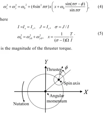
Here, we consider that the external torque is given for a spin period under the initial condition shown in Fig. 5. The angle between the position vector of the spin axis and the thruster direction is .

Nutation motion after thruster firing for one spin period can be written as follows:

2 2 2 2 0 0 sin( ) (4sin ) sin x y x x               _  _  , (4) where 2 2 2 0 0 0 , , / 1 , ( 1) x y z x y I I I J I J I T x I               . (5)

T is the magnitude of the thruster torque.

X

Y

X



Fig. 5 The initial condition of active nutation control.

As Eq. (4) shows, nutation motion is suppressed only when the second term on the right side is negative. From this equation, the nutation convergence condition can be driven as follows: 0 0 sin( ) 0 ( 1) sin( ) sin( ) 0 ( 1) sin( ) x x                   . (6)

Optimal jet timing exists when  , 1

* * sin( ) 1 2       . (7) When 1 * * if sin( ) 0 sin( ) 1 if sin( ) 0 sin( ) 1                . (8)

When thruster firing is began at _{ } *_{, nutation motion}

can be reduced most effectively. The  can be estimated

using the gyro outputs and _* _{is determined by the}

satellite inertia moment.

The control algorithm of the active nutation control software is shown in Fig. 6. The angular velocities perpendicular to the spin axis are measured by the gyro. The outputs of gyros are filtered by a band-path filter (BPF) and the coordinate is rotated to meet the optimal nutation control timing shown in Eq. (7) or Eq. (8). By this conversion, the optimal timing is sensed as the zero cross point of the BPF output.

1) If the BPF output exceeds the threshold, that is, nutation is large, the control flag is activated.

2) When the control flag is activated and the BPF output crosses the zero, the thrust command is activated. 3) After one spin period, put down the control flag and

thruster command. The spin period (Tsp0)is measured by the spin-type sun sensor.

Tsp0 Ancflag Thruster command BPF output *  

Fig. 6 The thrust timing of active nutation control.

3. Control System

In this section, the configuration of the attitude

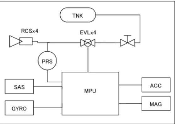
controller is shown. Figure 7 shows a block diagram of the attitude controller. This controller consists of a MPU, a 3D motion sensor (gyro, accelerometer, magnetometer), sun angle sensors and pressure sensors. Figure 8 shows the engineering model of the attitude controller for the SSSAT.

SAS GYRO RCSx4 PRS EVLx4 TNK MPU ACC MAG

Fig. 7 A block diagram of attitude control system. Table 1 Abbreviations for sub-components.

SAS Sun angle sensor

GYRO Gyro

ACC Accelerometer MAG Magnetometers

PRS Pressure sensor

EVL Electromagnetic valve

TNK Tank

Gyro Acc Mag

MPU

Fig. 8 The EM of the attitude controller.

MPU

PIC18F4580 (Microchip Technology Inc.) Multifunctional (ADC, DIO, CAN) 3D motion sensor

MAG3 (MEMSense)

Gyro+accelerometer+ magnetometer (3D)

Range (Gyro):400[deg/s]

Range (Acc): [G] 2

4. Hardware Simulation

4.1. Dynamics simulator and motion table

The motion table at ISAS/JAXA can simulate the 3D motion of a spacecraft. Using this motion table, we can check the validity of a control system with actual sensors. A block diagram of the hardware simulation system is shown in Fig. 10. A real-time computer (ARTLinux) calculates the attitude motion of the spacecraft, and motion table controller realizes the calculated attitude. The attitude controller calculates the control command.

The controller is attached on the motion table top (Fig. 11).

Fig. 9 The motion table.

ARTLinux Attitude Controller M/T M/T Controller Attitude data Sensor data Thruster command Attitude command M/T: Motion table Fig. 10 The hardware simulation system.

Fig. 11 The attitude controller attached on motion table.

4.2. Simulation Results

In this section, we show the results of the motion table experiment. The conditions of the experiment are shown in Eq.(9). 2 0.02267, 0.0120[kgm ] 0.539 1, 0.5 or 1.0[Hz] X Y Z I I I J I           . (9)

For simplicity, the experiments for rhumb line control and active nutation control were performed separately in this paper. In practice, the sequence of spin axis control is as follows:

1) Rhumb line control,

2) When nutation motion becomes large, active nutation control is performed,

4.2.1. Rhumb line control

Figure 12 and 13 show the time histories of the attitude

angles (pitch angle and yaw angle) for rhumb line

control. Figure 12 is the result of software simulation, and Figure 13 is the result of hardware simulation. Thruster delay is not considered in these simulations. These two cases have the same result. This proves that the sensors, the other hardware and control logic run properly.

0 5 10 15 20 -2 0 2 4 6 8 10 12 t [sec] ,  [d eg ]   Time[sec]

Fig.12 The pitch and yaw angles (sowtware simulation).

0 5 10 15 20 -2 0 2 4 6 8 10 12 t [sec]  ,  [d eg ]   Time[sec]

Fig.13 The pitch and yaw angles (hardware simulation).

-0.1 -0.05 0 0.05 0.1 -0.16 -0.14 -0.12 -0.1 -0.08 -0.06 -0.04 -0.02 0 X Y -0.2 -0.15 -0.1 -0.05 0 0.05 0.1 0.15 0.2 -0.3 -0.25 -0.2 -0.15 -0.1 -0.05 0 X Y

Fig. 14 The trajectory of angular momentum vector.

Figure 14 shows the results of hardware simulation when thrust delay exists. The left-hand figure shows the x and y components of the normalized angular momentum vector without delay compensation, and the right-hand figure shows the trajectory with delay compensation. The goal of this control is to shift the angular momentum vector along the Y axis. As these figures show, the angular momentum vector moves in the X direction without the delay compensator. On the other hand, the influence of delay is suppressed by the delay compensator. When the spin rate is large, the thrust delay causes serious control error. So delay compensation logic is very important for the spin-type spacecraft.

4.2.2. Active nutation control

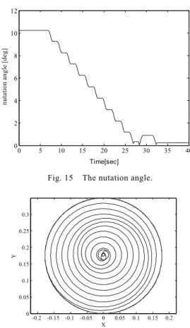
Here, we show the results of active nutation control hardware simulation. Figure 15 shows the time history of the nutation angle. The nutation angle is reduced by the control. Figure 16 shows the trajectory of the normalized spin axis vector. The spin axis approaches the center of the nutation motion. These results correspond with the results of the software simulations.

0 5 10 15 20 25 30 35 40 0 2 4 6 8 10 12 t [sec] nut at ion angl e [d eg] Time[sec]

Fig. 15 The nutation angle.

Fig. 16 The trajectory of spin axis vector.

5. Solar Sail Subpayload Satellite

The goals of the SSSAT were to demonstrate sail deployment and the attitude control. The attitude control logic before sail deployment is the same as the logic in section 2. However, after deployment, it becomes difficult

to control the attitude because of the large flexible

membrane. In this section, the new rhumb line control logic for the SSSAT is shown.

5.1. Specifications

Here, we show the specifications of the SSSAT. Figure 17 shows the pictures of the SSSAT. This satellite has a small cylindrical body and large membrane. The specifications of the SSSAT are:

Body: Cylinder (200h100[mm])

Membrane: 3.5[m]

Weight: 6[kg]

Thruster: Gas-liquid equilibrium thruster (800[mN]) x 4

(propellant: isobutene)

Solar cells: Thin a-Si(25[um])

-0.2 -0.15 -0.1 -0.05 0 0.05 0.1 0.15 0.2 0 0.05 0.1 0.15 0.2 0.25 0.3 X Y

Figure 18 shows a system block diagram of the SSSAT.

Fig. 17 The SSSAT.

Analog

Sensors

・Dust counter ・Membrane temp.

Camera

Analog & Digital

Digital MPU SAS × Gyro ACC, MAG TANK Thruster ACU CAN I/F MPU Memory DHU CAN I/F CAN bus JPEG coder Serial BAT PCU EPS + Latching valve SW S-TX S-RX COMM Digital MPU CAN I/F Serial Serial GPSR HCE 2 PRS

Fig. 18 A system block diagram of the SSSAT. Table 2 Abbreviations for the SSSAT system.

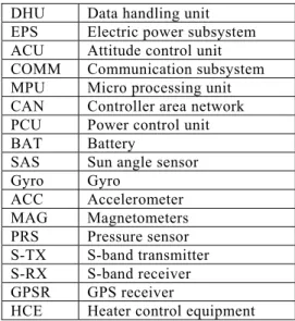
DHU Data handling unit

EPS Electric power subsystem

ACU Attitude control unit

COMM Communication subsystem

MPU Micro processing unit

CAN Controller area network

PCU Power control unit

BAT Battery

SAS Sun angle sensor

Gyro Gyro ACC Accelerometer MAG Magnetometers PRS Pressure sensor S-TX S-band transmitter S-RX S-band receiver GPSR GPS receiver

HCE Heater control equipment

5.2. Rhumb line control with membrane

In this section, we consider a simple satellite, as shown in Fig. 19. A jet is attached on oneside and it can give the

X-axis torque.

X

Y Z

Fig. 19 A simple solar sail satellite.

The rhumb line control of a satellite with membrane is the basically equal to the rhumb line control for a rigid body. The control torque can change the direction of the angular momentum of the satellite. However, nutation control of a satellite with membrane is very difficult. When the satellite is rigid, the active nutation control shown in section 2.2 is useful to attenuate the nutation motion. However, this active nutation control is difficult to apply to a satellite with membrane because the nutation motion is complicated due to the flexibility of the

membrane. The dumping of membrane can remove the

nutation passively, but it takes a long time to remove the nutation. Therefore, it is very important to prevent nutation from increasing.

In the case of a rigid satellite case, the nutation motion of the satellite can be easily estimated with the gyro output. However, it is very difficult to estimate the nutation motion of a solar sail satellite because the body motion is coupled with membrane motion. Many sensors on the membrane and complicated calculations are required to estimate the attitude motion completely. However, we can estimate the magnitude of nutation motion approximately with the body-mounted gyros.

When nutation motion is completely removed, 0



 _y

x 

 . In this case, the satellite body and membrane

rotate together around the Z-axis. If there is nutation,

0

, _y 

x 

 . As mentioned above, it is difficult to estimate

the nutation motion precisely, but we can assume that the larger the nutation become, the larger 2_x2_y is. In this paper, we propose the new rhumb line control method with gyro output.

In order to control nutation motion, the thrust firing timing is important. In the case of Fig. 19, thrust firing

when 0_x increases nutation motion. Here, we show

an example. Figure 20 shows the attitude motions of a solar sail satellite. Two cases are compared here. In both cases, the first pulse torque gives the nutation motion. The second torque timings are different. In case 1, the second

torque is given when _x0. In this case, second torque

increases the nutation motion. In case 2, the second torque

is given when _x0 and nutation motion is

successfully removed. The magnitude of _x is not

always an accurate index of nutaion motion. However, it is very useful information for suppressing nutation.

0 100 200 300 400 500 -0.02 -0.015 -0.01 -0.005 0 0.005 0.01 0.015 0.02 Time [sec] x [rad /s] 1st pulse 2nd pulse (case 2) 2nd pulse (case 1) Case 1 Case 2

Fig. 20 The angular velocity of the solar sail satellite.

Here, we summarize the new rhumb line control logic. Figure 21 shows the control logic. The point of this new control is that rhumb line control and nutation control are conducted at the same time.

1) The thruster firing time is calculated with the output of the spinning sun sensor. (normal rhumb line control logic).

2) If the control torque is expected to increase nutation motion, the command is canceled (Fig. 21(A)). Whether the command should be canceled or not is determined from the gyro output.

This logic is very simple, but it is useful for controlling the attitude of the solar sail satellite.

Angular velocity Rhumb line control window Thruster command (A) (B) (A) (B) x 

Fig. 21 The new rhumb line control logic for solar sail satellites.

Simulation results are shown in order to verify the advantage of this new control law. The following two cases are considered here.

Case1: Rhumb line control for a rigid satellite. Case2: New control law proposed in Fig. 21.

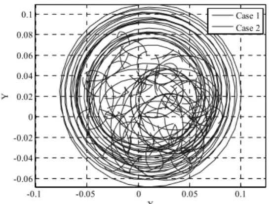
Figure 22 shows the histories of _x and Figure 23

shows the history of the thrust command. Figure 24 shows the total energy of the attitude motion. This energy indicates the magnitude of nutation motion and coupling of the body and membrane. (But it is impossible to observe the energy). In the case if flat spin, this energy becomes minimum. As these figures show, the proposed control logic effectively suppresses the nutation motion of the solar sail satellite. Figure 25 shows the trajectories of the normalized angular momentum vectors and Fig. 26 shows the spin axis trajectories. The angular momentum vectors can change in both cases, but attitude motions differ significantly. 0 200 400 600 800 1000 -0.02 -0.015 -0.01 -0.005 0 0.005 0.01 0.015 0.02 Time [sec] x [r ad/ s] Case 1 Case 2

Fig. 22 The histories of angular velocity.

0 200 400 600 800 1000 0 0.05 0.1 0.15 0.2 0.25 0.3 0.35 0.4 Time [sec] Nx [ N m ] Case 1 Case 2

Fig. 23 The histories of thrust command.

0 200 400 600 800 1000 4.39 4.395 4.4 4.405 4.41 Time [sec] E nergy [ J] Case 1 Case 2

Fig. 24 The histories of energy in attitude motion.

-5 0 5 10 15 x 10-3 0 0.005 0.01 0.015 0.02 X Y Case 1 Case 2

-0.1 -0.05 0 0.05 0.1 -0.06 -0.04 -0.02 0 0.02 0.04 0.06 0.08 0.1 X Y Case 1 Case 2

Fig. 26 The trajectories of spin axis.

6. Conclusion

This paper described the results of simulating the hardware of a small-spin-axis controller. The rhumb line control law and active nutation control law are implemented in the controller, and both controls achieve the desired performance. Furthermore, the new rhumb line control law for the SSSAT is discussed and its effectiveness is confirmed.

References

1) Kawaguchi, J., Morita, Y., Nakajima, T., Ishii, N., Hashimoto, T., Yamakawa, H., Hirokawa, E., Yasuda, S. and Balloon Group: Flight Test of the Rhumb Line Control System via Balloon, Proceedings of the 3rd Workshop on Astrodynamics and Flight Mechanics, 1993, pp.156-161.

2) Kawaguchi, J.: On the Simplified Recursive Formula of Rhumb Line Maneuvers with its Application to Identification of Directional Dispersion, Proceedings of the 3rd Workshop on Astrodynamics and Flight Mechanics, 1993, pp.194-199. 3) Yamamoto, T., Mori, O., Shida, M. and Kawaguchi, J.:

Development of Gas-Liquid Equilibrium Thruster for Small Satellite, International Symposium on Space Technology and Science, ISTS 2006-k-32, 2006.

4) Tsuda, Y., Mori, O., Nishimura. Y. and Kawaguchi,J.: Deployment Experiment of Thin Flexible Membrane Using Sounding Rocket for Future Solar Sail Mission, International Symposium on Space Technology and Science, ISTS 2004-c-11, 2004.

5) Nishimura, Y., Tsuda, Y., Mori, O. and Kawaguchi, J.: The Deployment Experiment of Solar Sail with Sounding Rocket, 55th International Astronautical Congress, IAC-04-A.5.10, 2004.