DYNAMICS OF MULTIPARAMETER SYSTEMS
ZIN ARAI∗, WILLIAM KALIES†, HIROSHI KOKUBU‡, KONSTANTIN MISCHAIKOW§, HIROE OKA¶, AND PAWE L PILARCZYKk
Abstract. A generally applicable, automatic method for the efficient computation of a database of global dynamics of a multiparameter dynamical system is introduced. An outer approximation of the dynamics for each subset of the parameter range is computed using rigorous numerical meth- ods and is represented by means of a directed graph. The dynamics is then decomposed into the recurrent and gradient-like parts by fast combinatorial algorithms and is classified via Morse decom- positions. These Morse decompositions are compared at adjacent parameter sets via continuation to detect possible changes in the dynamics. The Conley index is used to study the structure of isolated invariant sets associated with the computed Morse decompositions and to detect the ex- istence of certain types of dynamics. The power of the developed method is illustrated with an application to the two-dimensional, density-dependent, Leslie population model. An interactive vi- sualization of the results of computations discussed in the paper can be accessed at the website http://chomp.rutgers.edu/database/, and the source code of the software used to obtain these results has also been made freely available.
Key words.database, dynamical system, Conley index, Morse decomposition, Leslie population models, combinatorial dynamics, multiparameter system
AMS subject classifications. Primary: 37B35. Secondary: 37B30, 37M99, 37N25, 92-08.
1. Introduction. The global dynamics of a nonlinear system can exhibit struc- tures at all spatial scales, for example, the fractal structures associated to chaotic dynamics. The same phenomenon can occur with respect to the parameters, that is, global dynamical structures can change on Cantor sets in parameter space. From the point of view of scientific computation, only a finite amount of information can be computed, and therefore, any computational characterization of global dynamics of a multiparameter system can be expected to represent a dramatic reduction of informa- tion. Nevertheless, the computation of global dynamical information is an important
∗PRESTO, Japan Science and Technology Agency / Hokkaido University, Creative Research Initiative ”Sousei”, Sapporo 001-0021, Japan (email address: [email protected]). Partially supported by Grant-in-Aid for Scientific Research (No. 17740054), Ministry of Education, Science, Technology, Culture and Sports, Japan.
†Department of Mathematical Sciences, Florida Atlantic University, 777 Glades Rd, Boca Raton, FL 33431 (email address: [email protected]). Partially supported by NSF grant DMS-0511208 and DOE grant DE-FG02-05ER25713.
‡Department of Mathematics, Kyoto University, Kyoto 606-8502, Japan (email address:
[email protected]). Partially supported by Grant-in-Aid for Scientific Research (No.
17340045), Ministry of Education, Science, Technology, Culture and Sports, Japan.
§Department of Mathematics and BioMaPS, Hill Center-Busch Campus, Rutgers, The State University of New Jersey, 110 Frelinghusen Rd, Piscataway, NJ 08854-8019, USA (email address:
[email protected]). Partially supported by NSF grant DMS-0511115, by DARPA, and by DOE grant DE-FG02-05ER25711.
¶Department of Applied Mathematics and Informatics, Faculty of Science and Technology, Ryukoku University, Seta, Otsu 520-2194, Japan (email address: [email protected]). Par- tially supported by Grant-in-Aid for Scientific Research (No. 17540206), Ministry of Education, Science, Technology, Culture and Sports, Japan.
kCentre of Mathematics, University of Minho, Campus de Gualtar, 4710-057 Braga, Por- tugal and Department of Mathematics, Kyoto University, Kyoto 606-8502, Japan (website:
http://www.pawelpilarczyk.com/). Partially supported by the JSPS Postdoctoral Fellowship No.
P06039 and by Grant-in-Aid for Scientific Research (No. 1806039), Ministry of Education, Science, Technology, Culture and Sports, Japan.
1
problem for applications, which leads to the questions of how to characterize global dynamical structures and how to identify changes in these structures in practice. The fact that this is a nontrivial task has been made clear by the work of the dynamical systems community over the last century.
Identifying and classifying the qualitative properties of models over wide ranges of parameter values is of fundamental importance in many disciplines, and in particular it is of primary interest to many computational biologists [10]. The fact that most topics of interest in systems biology are dynamic in nature suggests the need for a comprehensive, yet efficient method for cataloging the global dynamics of nonlinear systems. In other words, a method is desired which computationally constructs a database of global dynamical behavior of a specific system over a range of parameters.
The starting point for our computational methods is Conley’s topological ap- proach to dynamics [2], which we review in the next section. The prior work in [1, 5, 9, 12, 24] has shown that Conley theory is an appropriate theoretical base for designing algorithms in computational dynamics. The purpose of this paper is to demonstrate that these ideas can be used to design an efficient computational frame- work for constructing databases of global dynamics of specific systems over multiple parameters. While the methods we propose are general, we illustrate them using a particular population model which we describe in Section 1.2.
1.1. Preliminary ideas. We restrict our attention to the setting of a multipa- rameter family of dynamical systems given by a continuous function
f:X×Λ3(x, λ)7→f(x, λ) =fλ(x)∈X (1.1) where the phase spaceX is a locally compact metric space and the parameter space Λ is a compact, locally contractible, connected metric space. Note that we do not assume thatfλ is a homeomorphism.
The fundamental structures in any dynamical system are the invariant sets. A setZ⊂X isinvariant atλ∈Λ iffλ(Z) =Z. Since we cannot perform computations at each parameter value independently, we are interested in considering sets which are invariant with respect to a subset of the parameter space. We use the notation F:X×Λ→X×Λ for the trivial extension of the system to include the parameters as explicit variables defined by
F(x, λ) = fλ(x), λ
= f(x, λ), λ
. (1.2)
For Λ0 ⊂ Λ we denote the restriction of F to X×Λ0 byFΛ0: X×Λ0 →X ×Λ0. Observe thatF =FΛ and thatfλ is readily identified withF{λ}. Moreover, given a setS⊂X×Λ we denote its restriction to Λ0 bySΛ0 :=S∩(X×Λ0). In particular, we often identifySλ ⊂X withS{λ}=Sλ× {λ}. In this language, a set S ⊂X×Λ isinvariant overΛ0 ifFΛ0(SΛ0) =SΛ0, which is an equivalent way to state that the setSλ is invariant at allλ∈Λ0.
We wish to identify and characterize a finite collection of invariant sets which determine the global, qualitative behavior of the dynamics. In addition, we need a method for comparing two invariant setsSλ0 andSλ1at distinct parameters. Deciding what sets to compute and how to compare them are the fundamental issues we attempt to address.
We emphasize that while the amount of information that can be computed is finite, this does not mean that we cannot detect or characterize dynamical structures that occur on arbitrarily small scales. For example, topological techniques can be
used to identify chaotic dynamics via a semiconjugacy onto a subshift of finite type, see [12]. Moreover, even though we cannot compute the dynamics at each parameter separately, this does not mean that we cannot obtain results which apply to every parameter value. Indeed, the methods we employ do compute mathematically rigorous global structures for invariant sets at all parameter values.
1.2. Model example. To provide perspective on the practicality and utility of our approach, we consider the two-dimensional version of an overcompensatory Leslie population modelg:R2×R4→R2 given by
x1
x2
7→
(θ1x1+θ2x2)e−φ(x1+x2) px1
,
where the fertility rates decay exponentially with population size. This model and its biological relevance is discussed in considerable detail in work of Ugarcovici and Weiss [25]. As indicated there, in view ofg(x, θ, p, φ) =φ−1g(φx, θ, p,1), the constant φmay be scaled arbitrarily, and thus it suffices to studyf:R2×R3→R2given by
(x, λ) =
x1
x2
,
θ1
θ2 p
7→f(x, λ) =
(θ1x1+θ2x2)e−0.1(x1+x2) px1
(1.3)
Furthermore, the detailed numerical studies of [25] indicate that this system exhibits a wide variety of different dynamical behavior, which suggests that it provides a meaningful test for the usefulness of the techniques introduced in this paper.
1.3. Outline of the paper. In the remainder of the paper we develop our method and apply it to the Leslie model. In Section 2 we introduce the dynamical structures which we utilize and review Conley theory. In Section 3 we introduce a method for building a combinatorial representation of the dynamics and a means of comparing the computed structures at different parameters. In Section 4 we address the question of efficient computational algorithms based on rectangular grids in X and Λ. In Section 5 we describe a database computed with our methods for the model example introduced in Section 1.2 withp= 0.7 andθ1, θ2varying in selected ranges, and we show how this database can be queried for various dynamical properties.
Finally, in Section 6 we briefly mention a result of similar computations where all three parameters are varied.
2. Review of Conley theory. Recall that a compact set N ⊂ X×Λ0 is an isolating neighborhoodforFΛ0 if
Inv (N, FΛ0)⊂intX×Λ0(N)
where Inv (N, FΛ0) denotes the maximal invariant set inNunderFΛ0, and intX×Λ0(N) denotes the interior ofN with respect to the subspace topology onX×Λ0. Isolating neighborhoods are computable and hence provide a means of identifying invariant sets. In particular, an invariant set SΛ0 ⊂ X ×Λ0 is an isolated invariant set if SΛ0 = Inv (N, FΛ0) for some isolating neighborhoodN.
As indicated in [2, 15], the space of isolated invariant sets is a sheaf. More precisely, ifN is an isolating neighborhood forF =FΛ andS= Inv (N, F), then for any Λ0⊂Λ,NΛ0 is an isolating neighborhood for FΛ0 andSΛ0 = Inv (NΛ0, FΛ0). In particular, for anyλ∈Λ,S{λ}⊂X× {λ}is an isolated invariant set forF{λ}:X× {λ} →X× {λ}andSλ⊂X is an isolated invariant set forfλ:X →X.
To simplify the presentation and analysis, throughout this paper we make use of the following assumption and establish the following notation.
A1: There exists a compact set B ⊂ X ×Λ which is an isolating neighborhood for F. Its maximal invariant set is denoted by S :=
Inv (B, F).
Using the sheaf property of isolated invariant sets,SΛ0 denotes the restriction of S toX×Λ0, which is an isolated invariant set forFΛ0 if Λ0is compact. As indicated above, we are interested in understanding the structure of Sλ for all λ∈ Λ, and we make use of two essential ideas due to Conley [2]: Morse decompositions and the Conley Index.
2.1. Morse decompositions. Recall that a Morse decomposition of SΛ0 is a finite collection
M(SΛ0) ={MΛ0(p)⊂SΛ0 |p∈ PΛ0}
of disjoint isolated invariant sets ofFΛ0, calledMorse sets, which are indexed by the set PΛ0 on which there exists a strict partial order>Λ0, called anadmissible order, such that for every (x, λ) ∈ SΛ0 \S
p∈PMΛ0(p) and any complete orbit γ of FΛ0
through (x, λ) inSΛ0 there exist indicesp >Λ0 qsuch that under FΛ0 ω(γ)⊂MΛ0(q) and α(γ)⊂MΛ0(p).
Morse decompositions provide a coarse but global description of the dynamics onSΛ0. Remark 2.1. With regard to the construction of a database for global dynamics, we make several important observations concerning Morse decompositions, see [2, 13].
1. Morse decompositions of SΛ0 are not unique. They can often be refined or coarsened, and many systems have no finest Morse decomposition.
2. The empty set can be a Morse set.
3. Every structure withinSΛ0 that is associated with recurrent dynamics, e.g. a fixed point, a periodic orbit, or chaotic dynamics, must lie in some Morse set.
Away from the Morse sets the dynamics is gradient-like and the direction of trajectories is captured by an admissible partial order.
4. Given a Morse decomposition, there is a unique minimal admissible partial order called theflow-defined order. Any extension of the flow-defined order which maintains a strict partial order produces an admissible order.
5. Consider a Morse decompositionM(SΛ0) ={MΛ0(p)⊂SΛ0 |p∈ PΛ0}ofSΛ0
with admissible order>Λ0. If Λ1⊂Λ0, then the collection of sets {MΛ1(p)⊂SΛ1 |p∈ PΛ0},
whereMΛ1(p) :=MΛ0(p)∩(X×Λ1), is a Morse decomposition ofSΛ1 under
FΛ1 with the same admissible order.
Observe that sincePΛ0is a strict partially ordered set, a Morse decomposition can be represented as an acyclic directed graph MG(Λ0) called theMorse graph overΛ0. The elements of the index setPΛ0, which naturally correspond to the Morse sets, are the vertices of the Morse graph over Λ0, and the edges of the Morse graph over Λ0are the minimal order relations which through transitivity generate>Λ0. In other words, forp, q∈ PΛ0 there is a directed edgep→qin MG(Λ0) ifp >Λ0 qand there doesnot existr∈ PΛ0 such thatp >Λ0 r >Λ0 q.
Computationally, we obtain Morse decompositions indirectly, and often it can be established by further computation that a Morse set is empty. In that case, such a set can be removed from the Morse decomposition as described by the following proposition whose proof follows directly from the definition of a Morse decomposition.
Proposition 2.2. Consider a Morse decompositionM(SΛ0) =
MΛ0(p)⊂SΛ0| p∈ PΛ0 of SΛ0 with admissible order>. AssumeMΛ0(p0) =∅. Then
M0(SΛ0) :={MΛ0(p)⊂SΛ0 |p∈ PΛ0\ {p0}}
is a Morse decomposition ofSΛ0 and an admissible order is given by >0 where for all p, q∈ PΛ0\ {p0}we have p >0 qif and only if p > q.
From Proposition 2.2, if MG(Λ0) is the Morse graph over Λ0 corresponding to M(SΛ0), then MG0(Λ0), the Morse graph over Λ0 corresponding to M0(SΛ0), has vertices PΛ0 \ {p0} and has an edgep→q if eitherp→q is an edge in MG(Λ0) or p → p0 → q are edges in MG(Λ0). The simplified Morse graph MG0(Λ0) is called a trivial reduction of MG(Λ0). Whenever possible, we work with a trivial reduction of a Morse graph. The possibility that a Morse set is trivial can be detected via the Conley index which is described in the next section.
2.2. The Conley index. As explained in Section 3, computational methods exist to find Morse decompositions, see [1]. The Conley index, which is an algebraic topological invariant of isolated invariant sets, is used to understand the structure of the dynamics within a Morse set.
To explain the index we begin by considering an arbitrary continuous mapg:Z → Z on a locally compact metric space and a pair of compact setsN = (N1, N0) such that N0⊂N1⊂Z. Consider the pointed quotient space N1/N0,[N0]
obtained by collapsingN0 to a single point [N0]. DefinegN: N1/N0,[N0]
→ N1/N0,[N0] by gN(x) =
g(x) if x, g(x)∈N1\N0
[N0] otherwise.
The pairN= (N1, N0) is anindex pairif the mapgN is continuous and cl (N1\N0) is an isolating neighborhood [21].
The following two facts about index pairs are most relevant and can be found in [2, 13].
1. For any isolated invariant set K, there exists at least one index pair N = (N1, N0) such thatK= Inv (cl (N1\N0), g).
2. For any isolated invariant set K, there can exist many index pairs which isolateK.
The first fact implies that for any Morse set MΛ0(p) for the system FΛ0 there exists an index pairN = (N1, N0) such that the induced mapFΛ0,N: N1/N0,[N0]
→ N1/N0,[N0]
is a continuous function andMΛ0(p) = Inv cl (N1\N0), FΛ0
. Passing to homology leads to a family of group endomorphisms
FΛ0,N∗:H∗ N1/N0,[N0]
→H∗ N1/N0,[N0]
. (2.1)
The second fact allows for different choices of index pairs which can lead to different group endomorphisms. Thus, to define the Conley index of an isolated invariant set, such as a Morse set MΛ0(p), one must consider equivalence classes of these group endomorphisms [13]. In constructing our database, we do not utilize the full Conley index; instead, we store a weaker invariant, namely the nonzero eigenvalues
ofFΛ0,N∗restricted to the torsion-free part ofH∗ N1/N0,[N0]
. This weaker invariant is chosen because these eigenvalues are readily computed and compared.
Remark 2.3. With regard to the construction and interpretation of the database, there are several important observations about the index to be made, see [13].
1. If the Conley index is trivial, then the map FΛ0,N∗ is nilpotent. This im- plies that the eigenvalues of FΛ0,N∗ restricted to the torsion-free part of H∗ N1/N0,[N0]
are all zero.
2. The empty set is an isolated invariant set with trivial Conley index. Thus, if there are nonzero eigenvalues of FΛ0,N∗ restricted to the torsion-free part of H∗ N1/N0,[N0]
, thenMΛ0(p)6=∅.
3. There exist nontrivial isolated invariant sets with trivial Conley index. For example, consider the logistic mapgλ(x) =λx(1−x),λ∈[1,4], and an index pairN = (N1, N0) = [−1,2],{−1,2}
. The index mapFN∗ is nilpotent, but clearlySλ= Inv (N1\N0, gλ)6=∅.
4. The Conley index can be used to reconstruct some of the structure of the dynamics of the associated isolated invariant set. In particular, under appro- priate conditions the Conley index can be used to conclude the existence of fixed points, periodic orbits, and chaotic dynamics.
5. Suppose Λ1 ⊂Λ0 are both contractible. If MΛ0(p) is a Morse set, or indeed any isolated invariant set, then the nonzero eigenvalues of the torsion-free part of any index mapFΛ0,N∗ are identical to the nonzero eigenvalues of the torsion-free part of any index map FΛ1,N∗ for the set MΛ1(p) = MΛ0(p)∩
(X×Λ1).
2.3. Conley-Morse graphs. We are now in a position to describe the funda- mental element of our database. Let Λ0⊂Λ and letM(SΛ0) ={MΛ0(p)⊂SΛ0 |p∈ PΛ0} be a Morse decomposition ofSΛ0with admissible order>Λ0. TheConley-Morse graph overΛ0ofM(SΛ0) is denoted by CMG(Λ0) and consists of MG(Λ0), the Morse graph over Λ0with the additional information of the nonzero eigenvalues of the torsion-free part of the index map of each Morse set assigned to the associated node. We present this information by labeling each node in the following format.
pk: n→ {∗}
denotes the fact that thek-th Morse set has nonzero eigenvalues{∗}on then-th level of homology. If thek-th Morse set has no nonzero eigenvalues then we write
pk: 0 .
An example of how this information can be used to describe the structure of the dynamics is given in Proposition 5.8.
As described in Sections 3 and 4, we compute the Conley-Morse graphs over distinct fixed subregions of parameter space. This raises the question of how to relate the resulting Conley-Morse graphs. One answer is provided in the following definition.
Definition 2.4. Assume A1. Let Λ0,Λ1⊂Λ be such that Λ0,1:= Λ0∩Λ1 is a nonempty, contractible set. Let
M(SΛi) ={MΛi(p)⊂SΛi |p∈ PΛi}
fori= 0,1 be Morse decompositions with admissible orders>i. The associated Morse graphs MG(Λ0) over Λ0 and MG(Λ1) over Λ1 are equivalentif there exists an order
preserving bijectionι: (PΛ0, >0)→(PΛ1, >1) such that MΛ0(p)∩(X×Λ0,1) =MΛ1 ι(p)
∩(X×Λ0,1).
The continuation property of the Conley index [2] implies that if MG(Λ0) and MG(Λ1) are equivalent via the order preserving bijection ι: (PΛ0, >0)→ (PΛ1, >1), then the Conley-Morse graphs CMG(Λ0) and CMG(Λ1) are also equivalent, that is, the nonzero eigenvalues associated to corresponding Morse sets are identical.
3. Combinatorial representation of dynamics. Conley-Morse graphs are the key elements of information stored in our database. In this section we describe a general procedure for computing these graphs. We begin by describing a means of combinatorializing the dynamics.
Recall [17] that agridon a metric spaceZis a collectionZ of nonempty, compact subsets ofZ with the following properties:
(a) Z=S
G∈ZG, (b) G= cl int (G)
for allG∈ Z,
(c) G∩int (H) =∅for allG6=H∈ Z, and
(d) ifK⊂Z is compact, then{G∈ Z |G∩K6=∅}is a finite set.
The grid Z has the simple intersection property if G, H ∈ Z and G∩H 6= ∅ im- plies that G∩H is contractible. The diameter of a grid is defined by diam (Z) :=
supG∈Zdiam (G), and therealization map|·|is a function from subsets ofZto subsets ofZ defined by |A|:=S
A∈AA. GivenY ⊂Z, define Z(Y) :={G∈ Z |int (G)∩Y 6=∅}.
For the remainder of the paper, X and Q denote grids with the simple intersection property onX and Λ, respectively. Observe thatX × Qis a grid forX×Λ. As shown in [9], givenδ >0 we can choose grids such that diam (X)< δ and diam (Q)< δ.
A combinatorial multivalued map F: Z −→→ Z assigns to each element G ∈ Z a finite (possibly empty) subset F(G) of Z. Important for efficient computation is the observation that a combinatorial multivalued map F: Z −→→ Z is equivalent to a directed graph with vertices Z and directed edges (G, H) whenever H ∈ F(G). A directed graph isclosed if each vertex is both the head of at least one edge and the tail of at least one edge.
We use combinatorial multivalued maps on the gridX as a means to discretize and combinatorially approximate the dynamics off. For a more detailed description see [9]. Fixλ∈Λ and a compact setBλ⊂X. We relatefλ|Bλ:Bλ→X to the com- binatorial multivalued mapFλ:X(Bλ)−→→ X by requiring thatFλouter approximates fλ in the following sense [24]. A multivalued mapFλ:X(Bλ)−→→ X is called an outer approximationoffλrestricted to|X(Bλ)|iffλ(G)⊂int |Fλ(G)|
for allG∈ X(Bλ).
The property of being an outer approximation is the key to approximating the dynamics off combinatorially. Since we can only perform a finite number of compu- tations, we cannot computeFλindividually for eachλ∈Λ. Recall that we have made the assumptionA1so that the compact setB ⊂X×Λ is an isolating neighborhood forF, andS = Inv (B, F). From the point of view of the computational algorithms it is more convenient to additionally assume the following condition similar in spirit to A1. As it is made clear via Remarks 4.3 and 5.2, these two assumptions are computationally compatible.
A10: For each grid elementQ∈ Qthe set BQ :=X S
λ∈QBλ has the property thatSQ = Inv |BQ| ×Q, FQ
.
Now for eachQ∈ Qwe consider a multivalued mapFQ:BQ−→→ X with the prop- erty that
f(G, Q)⊂int |FQ(G)|
(3.1) for all G ∈ BQ. Observe that if λ ∈ Q, then FQ is an outer approximation of fλ
restricted to|BQ|. We organize the collection ofFQ via the following definition. Set B:= [
Q∈Q
BQ× {Q}
⊂ X × Q.
AcombinatorializationofFon|B|is the combinatorial multivalued mapF:B −→→ X ×Q defined by
F(G, Q) =FQ(G)× {Q}.
Note thatF is composed of a collection of outer approximations of eachFQ.
The following proposition indicates how outer approximations are used to capture invariant sets.
Proposition 3.1. Suppose A10 holds and F is a combinatorialization of F on |B|. Let Q∈ Q, and suppose Y ⊂ BQ. If N is the maximal subset ofY such that the restrictionFQ:N −→→ N is closed, then
Inv (|Y| ×Q, FQ) = Inv (|N | ×Q, FQ).
Proof: Let (x, λ) ∈ Inv (|Y| ×Q, FQ) and choose any G ∈ Y that contains x. Let γx be a complete orbit ofFQ through (x, λ) in Inv (|Y| ×Q, FQ). SinceFQ satisfies (3.1), there exists a sequence {Gn} in Y with G0 = G and Gn+1 ∈ FQ(Gn) such that γx(n) ∈ Gn×Q for all n ∈ Z. Therefore G ∈ N, because it lies in a closed subgraph{Gn}of Y, which implies that{Gn} ⊂ N, and thusγx ⊂ |N | ×Q. Hence (x, λ)∈Inv (|N | ×Q, FQ). This implies that Inv (|Y| ×Q, FQ)⊂Inv (|N | ×Q, FQ).
Since the opposite inclusion is trivial, this concludes the proof.
Proposition 3.1 states that the maximal invariant set is captured by the largest closed subgraph of a combinatorialization. We have already commented that grids of arbitrarily small diameter exist in general. IfSQis the largest closed subgraph ofBQ, then it follows from the results in [9] that|SQ|converges to SQ in Hausdorff metric as the grid diameters of X and Q tend to zero and the amount of overestimate in the computation of the outer approximation of the image of f by F tends to zero, see Theorem 5.8 and Lemma 7.6 of [9]. We do not provide details here, because even though the convergence results prove that the maximal invariant set can be approximated arbitrarily closely if computations are performed on a sufficiently fine scale, in practice we fix a priori a finest resolution in the phase space and the parameter space with which we do our computations.
3.1. Constructing Conley-Morse graphs. Recall that we have assumed that F satisfiesA1. In addition, for the remainder of this section we assume that the set B and the gridX are chosen in such a way thatA10 is satisfied.
A natural starting point for examining the global structure of both a dynam- ical system and a directed graph is to look for recurrence. The recurrent set of FQ:SQ−→→ X is defined by
RQ:={G∈ SQ|there exists a nontrivial path from Gto Gin SQ},
where a nontrivial path is any path of non-zero length, including the case a loop from a vertex to itself. The recurrent setRQ is naturally partitioned into equivalence classes{MQ(p)|p∈ PQ}called combinatorial Morse setsaccording to the following equivalence relation:
G'H if and only if there exists a path inFQ from Gto H and a path inFQ from H toG.
Since every node inSQ that lies on a cycle is an element ofRQ, we can define a strict partial order on the indexing set PQ by setting p >Q q if there existG ∈ MQ(p), H ∈ MQ(q), and a path fromGto H in FQ.
Observe that this construction implies that a combinatorial Morse decomposition can be represented as a directed graph. Let MG(FQ) denote the acyclic directed graph with vertices consisting of the elements ofPQ and the minimal set of directed edges p→qwhich generatep >Qqunder transitivity. The following proposition states that given a combinatorial Morse decomposition for an outer approximationFQ, there is a Morse decomposition ofFQ such that MG(FQ) is the Morse graph overQfor the Morse decomposition.
Proposition 3.2. Assume A1 and A10 are satisfied. Let Q ∈ Q and let {MQ(p)|p∈ PQ} be the set of combinatorial Morse sets for FQ. If FQ MQ(p)
⊂ BQ for allp∈ PQ, then the acyclic directed graphMG(FQ)which represents the com- binatorial Morse sets is a Morse graph over Q for the Morse decomposition of SQ
defined by
M(SQ) :={Inv (|MQ(p)| ×Q, FQ)|p∈ PQ}. Moreover, each|MQ(p)| is an isolating neighborhood forInv|MQ(p)|.
Proof: By [9, Theorem 4.1], we know that|MQ(p)| ×Qis an isolating neighborhood forFQ, and by [9, Corollary 4.2],
M(SQ) :={MQ(p) := Inv (|MQ(p)| ×Q, FQ)|p∈(PQ, >Q)}
is a Morse decomposition ofSQ.
Remark 3.3. Observe that Proposition 3.2 implies that once an appropriate combinatorialization of F has been computed, then for each Q ∈ Qa Morse graph MG(FQ) overQis determined which can be associated to a true Morse decomposition M(SQ) for FQ, and this in turn provides a Morse decomposition M(Sλ) forfλ for
eachλ∈Q.
The algorithms used to compute the Conley-Morse graphs are discussed in greater detail in Section 4. For the moment we remark that we use the algorithm presented in Section 2.2 of [1] to compute the Morse graph MG(FQ). There are a variety of algorithms for determining index pairs, see [8, 18, 19, 24], and in this paper we adopt the approach of [19], see Remark 4.3. For systems defined in Rn and simplicial or rectangular grids, there exist algorithms to compute the induced map on homology [8, 14, 20]. Hence for eachQ∈ Qthe Conley-Morse graph CMG(FQ) can be determined in a fairly general setting.
3.2. Comparing Conley-Morse graphs. We now turn to the question of com- paring the dynamical information over different parameter regions via Conley-Morse graphs. Recall that we assume that the grid Qhas the simple intersection property.
Furthermore, we continue to assume that A1andA10 are satisfied. We also assume that CMG(FQ) has been computed for eachQ∈ Q. We begin with a few definitions.
Definition 3.4. To eachQ ∈ Q, there is an associated CMG(FQ). Consider Q0, Q1 ∈ Qsuch thatQ0∩Q1 6=∅. Theclutching graph J(Q0, Q1) is defined to be the bipartite graph with verticesPQ0∪ PQ1 (the union of the vertices from MG(FQ0) and MG(FQ1)) and with an edge (p, q)∈ PQ0× PQ1 ifMQ0(p)∩ MQ1(q)6=∅.
Observe that if every vertex inPQ0in the clutching graphJ(Q0, Q1) has a unique edge, then we can define theclutching function
ιQ1,Q0:PQ0 → PQ1
byιQ1,Q0(p) :=qfor each edge (p, q) ofJ(Q0, Q1).
Definition 3.5. Consider the set of Conley-Morse graphs over the grid elements of the parameter space, i.e.{CMG(FQ)|Q∈ Q}. LetQ0, Q1∈ Qsuch thatQ0∩Q16=
∅. If the clutching functionιQ1,Q0:PQ0→ PQ1 is defined and gives a directed graph isomorphism from MG(FQ0) to MG(FQ1), then we say that the Conley-Morse graphs overQ0andQ1, CMG(FQ0) and CMG(FQ1), areequivalent. The equivalence classes of{CMG(FQ)|Q∈ Q}with respect to the transitive closure of this relation are called continuation classes.
Remark 3.6. We require thatιQ1,Q0 generate a directed graph isomorphism as opposed to the weaker condition thatιQ1,Q0 be a bijection, because differences in the partial order may indicate a difference in the dynamics.
Proposition 3.7. Assume A1 and A10 are satisfied. Let Q0, Q1 ∈ Q such that Q0∩Q1 6=∅. If the clutching function ιQ1,Q0:PQ0 → PQ1 is a directed graph isomorphism then there exists a Morse decomposition
M(SQ0∪Q1) ={MQ0∪Q1(r)|r∈ PQ0∪Q1}
with admissible order >Q0∪Q1 such that its restriction is the same as the Morse de- composition M(SQi)over Qi for each i= 0,1. Specifically, there is a natural corre- spondenceπi: PQ0∪Q1→ PQi such that
MQi πi(r)
=MQ0∪Q1(r)∩(X×Qi)for anyr∈ PQ0∪Q1,
and >Q0∪Q1 agrees with >Qi through the identification. Furthermore, the nonzero eigenvalues associated to the index maps for pairs of corresponding Morse setsMQ0(π0(r)) andMQ1(π1(r))are the same.
Proof: Define
PQ0∪Q1={(p, q)∈ PQ0× PQ1 |q=ιQ1,Q0(p)},
and the natural correspondenceπi:PQ0∪Q1 → PQi. Then one can introduce a well- defined partial order >Q0∪Q1 onPQ0∪Q1 from the isomorphic partial order >Qi on PQi, andπi becomes an order-preserving isomorphism.
Now define
MQ0∪Q1(r) =MQ0 π0(r)
∪MQ1 π1(r) .
It follows from the construction that the collection{MQ0∪Q1(r)|r∈ PQ0∪Q1}forms a Morse decomposition overQ0∪Q1. The result now follows from the sheaf property of Morse decompositions and the continuation property of the Conley index.
Proposition 3.7 implies that if CMG(FQ0) and CMG(FQ1) belong to the same continuation class then there is a path in the parameter space along which the un- derlying Morse decompositions are related by continuation, and the Conley indices of the corresponding Morse sets are isomorphic.
Remark 3.8. It is important to note that belonging to the same continuation class is a weak equivalence relation. In particular, it is possible that λ0, λ1 ∈Q∈ Q and yetSλ0 andSλ1 are not topologically conjugate. Thus, membership in the same continuation class does not imply equivalence on the level of conjugacy. Heuristically, this is because we are studying the dynamics on the level of the grid elements and differences in the dynamics that lie below this scale cannot be observed. Similarly, it is possible that CMG(FQ0) and CMG(FQ1) lie in different continuation classes, but the dynamics offλ0 onSQ0 forλ0∈Q0andfλ1 onSQ1 forλ1∈Q1are topologically equivalent. To see that this is the case considerλi=λ∈Q0∩Q1, but CMG(FQ0) and CMG(FQ1) do not belong to the same continuation class. The heuristic explanation for this is that topological conjugacy is independent of the size of the dynamic struc- tures, but the construction ofFclearly depends on the size of the grid decomposition.
Finally, it is possible to construct examples in which CMG(FQ0) and CMG(FQ1) belong to the same continuation class and Q0∩Q16=∅, butιQ1,Q0 is not a directed graph isomorphism, or evenιQ1,Q0 may not be defined. This situation can arise from lack of resolution in either the phase space or parameter space. In fact, in practice (see Section 4.6) we employ a local subdivision algorithm that in principle reduces – but does not necessarily eliminate – the occurrence of phenomenon of this type.
The thesis of this paper is that, given grids for the phase space and parameter space, a useful database for the global dynamics is a list of the continuation classes and their relative connectivity. To be more precise we introduce the following notion.
Definition 3.9. AssumeA1andA10 are satisfied. The associatedcontinuation graphCG(F) is a graph whose vertices are the continuation classes
CMG(j),Q(j)
|j= 1, . . . , J
whereQ(k)⊂ Qis the set of parameter boxes associated with the k-th continuation class and CMG(k) = CMG(FQ) for some Q ∈ Q(k). Note that all Conley-Morse graphs CMG(FQ) over Q ∈ Q(k) are isomorphic. There is an edge between the j- th and k-th vertices in CG(F) if there exist Q ∈ Q(j) and Q0 ∈ Q(k) such that Q∩Q0 6=∅.
The continuation graph is our database. Of course, additional, problem specific information can also be stored. However, as will be indicated in the context of the density dependent Leslie model, this database provides an extremely compressed yet useful means of describing the global dynamics over a broad range of parameter values.
We return to these issues when we use the database to investigate the Leslie model.
4. Building the database using rectangular grids. The results of Section 3 indicate how a combinatorialization of F leads to a database. In this section we describe how a combinatorialization can be effectively computed, including details of selected computational aspects of the method.
The optimal choice of a suitable grid is determined by the structure ofX, Λ, and B⊂X×Λ. For many applications Λ⊂Rmis a rectangular region,X =Rn, andB
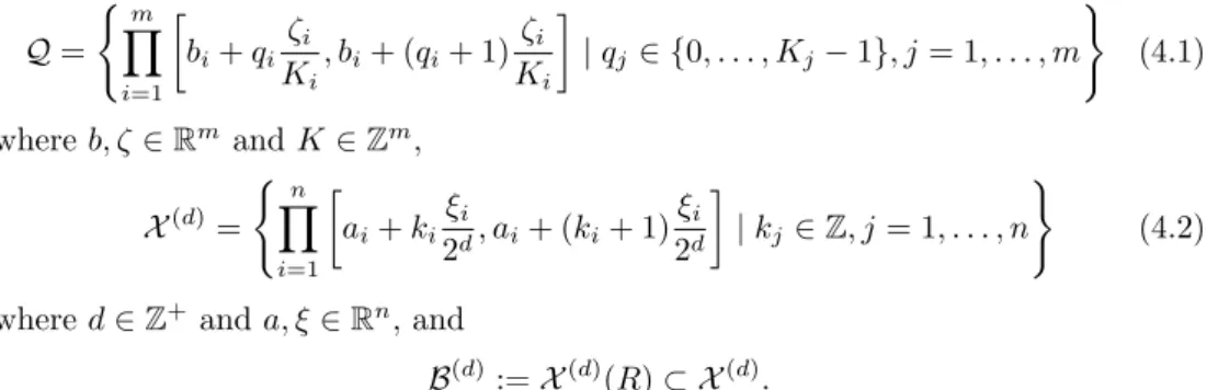
is also a rectangular region, that is,B =R×Λ for some rectangular regionR⊂Rn. For convenience, we make this assumption, i.e.Bλ=Rfor allλ∈Λ, throughout the rest of this paper. This leads to the use of a pair ofrectangular grids
Q= (m
Y
i=1
bi+qi
ζi
Ki
, bi+ (qi+ 1)ζi
Ki
|qj ∈ {0, . . . , Kj−1}, j= 1, . . . , m )
(4.1) whereb, ζ∈RmandK∈Zm,
X(d)= ( n
Y
i=1
ai+ki
ξi
2d, ai+ (ki+ 1)ξi
2d
|kj ∈Z, j= 1, . . . , n )
(4.2) whered∈Z+ anda, ξ∈Rn, and
B(d):=X(d)(R)⊂ X(d).
The choices ofKandddefine the accuracy of computations, and the choices ofa,b,ξ andζare determined by the regions one wishes to study. The parameterdallows for the use of an iterative multiscale method described later that is essential for efficient computation of the dynamics.
4.1. Constructing an outer approximation. For eachQ∈ Q we construct an outer approximationFQ(d):B(d)−→→ X(d)as follows. For each grid elementG∈ B(d), interval arithmetic [16] is used to compute a rectangular box β(G) which contains the image f(G, Q). More precisely, the edges of the rectangular grid elementG×Q (which are intervals) are inserted directly into the formula forf in place of correspond- ing variables, and the value of f(G, Q) is evaluated using interval arithmetic which provides a rigorous result in the form of a product of intervals. For each G∈ B(d) define
FQ(d)(G) :=
H ∈ X(d)|H∩β(G)6=∅
and observe that f(G, Q) ⊂ int|FQ(d)(G)|, see Figure 4.1. Thus, FQ(d) is an outer approximation as defined in (3.1).
Fig. 4.1. A rigorous enclosure of the image of each grid box (dark gray) is computed with interval arithmetic (indicated by the dotted line), and then covered by grid boxes (light gray).
Having described the construction of FQ(d):B(d)−→→ X(d), we turn to the need for a multiscale approach. Observe that the number of grid elements in B(d) is 2nd, and hence the size of the graph of FQ grows exponentially as a function either of discretization size or dimension of the problem. However, we are only interested in the largest closed subgraph ofFQonB(d), and thus we only use the restriction ofFQ
toSQ(d), where|SQ(d)| ×Qcovers InvBQ which is often a small subset ofBQ.
4.2. Iterative multiscale identification of the invariant set. To avoid un- necessary computation, we use the following iterative multiscale approach motivated by [7]. Letd0, d1, . . . , d` be an increasing sequence of positive integers. Fix Q∈ Q.
ConstructFQ(d0):B(d0)−→→ X(d0). Following the algorithms in [1] we compute the max- imal closed directed graph SQ(d0) in FQ(d0). Define Y(d1) ⊂ B(d1) to be the grid for
|SQ(d0)|. Construct FQ(d1):Y(d1)−→→ X(d1). We repeat the construction of SQ(di) and FQ(di): Y(di)−→→ X(di) until i = l. Note that since we assume A10, Proposition 3.1 implies that Inv |S(d`)| ×Q
= Inv |BQ(d0)| ×Q .
Example 4.1. To put the above construction into perspective consider the Leslie model (1.3) where we fixp= 0.7. Set
Λ :={(θ1, θ2)∈[8,37]×[3,50]},
R:= [−0.001,320.056]×[−0.001,224.040] for allλ∈Λ.
The grid Q in Λ is given by (4.1) with m = 2, b1 = 8, b2 = 3, ζ1 = 29, ζ2 = 47, and K1 = K2 = 50, while the grids X(d) in X = R2 are given for d = 1, . . . ,12 by (4.2) withn = 2, a1 =a2=−0.001,ξ1 = 320.057 and ξ2 = 224.041. Figure 4.2 indicates the evolution of the sets SQ(d) for d = 1, . . . ,12, where Q∈ Q is given by (q1, q2) = (20,33) in (4.1).
Remark 4.2. Observe that the diameter of |FQ(d)(G)|depends on the diameter ofβ(G), which in turn is dependent both on the diameter ofGandQ. Currently, we fix the gridQand then iteratively refineX(d). Thus, the size ofQ∈ Qputs an upper bound on the number of iterative steps that lead to a useful refinement of the outer approximation FQ(d):Y(d)−→→ X(d). A more sophisticated approach would involve an iterative method for both the phase space and the parameter space.
Remark 4.3. By Proposition 3.1, SQ ⊂ |SQ(di)| ×Q fori = 0, . . . , l. Moreover, sinceSQ(di) is the maximal closed subgraph, and combinatorial Morse sets are closed subgraphs, each combinatorial Morse setMQ(p) forp∈ PQ is contained inSQ(di) for each i= 0, . . . , `. If F MQ(p)
⊂ BQ for allp∈ PQ, then by Proposition 3.2, the neighborhoods|MQ(p)|isolate Morse sets in a Morse decomposition ofSQ. Moreover, since Morse sets are recurrent, the conditionF MQ(p)
⊂ BQ implies that FQ FQ(MQ(p))\ MQ(p)
∩ MQ(p) =∅, (4.3)
where FQ:X → X is an outer approximation. As described in the next section, this allows us to readily compute the Conley index of Inv (|MQ|). If the condition F MQ(p)
⊂ BQ is not satisfied, then we cannot compute the index without extend- ing our computation ofFQ outside ofBQ, and this situation is reported in the output
of our computations.
4.3. Conley-Morse graph computation. Given FQ(d`): SQ(d`)−→→ X(d`) the al- gorithm in [1, Section 2.2] is used to compute the Morse graph MG(FQ), where FQ := FQ(d`). To produce the Conley-Morse graph over Q requires the computa- tion of the Conley indices of each Morse set. This is done using the algorithms in [14, 20] and the easy observation that if MQ(p) is a combinatorial Morse set for FQ and the condition (4.3) is satisfied for FQ: MQ(p)∪ FQ(MQ(p))−→→ X, then
MQ(p)∪ FQ(MQ(p)),FQ(MQ(p))\ MQ(p)
is a combinatorial index pair as in
Fig. 4.2. Computation of S(dQi) by means of gradual refinements. In the first row, the lines indicate the subdivision of the regionX into4n boxes forn= 1, . . . ,4. No more lines are added in the second row to keep the picture clear. The third row shows a magnified fragment of the regionSQ(di)with the lines corresponding to those in the second row. Parameter boxQcoordinates:
(q1, q2) = (20,33).
[19, 20]. In practice, there are memory constraints associated with these algorithms for computing the Conley index. In the computations performed for this paper we did not attempt to compute the Conley index if the index pairs generated contained more than 400,000 boxes.
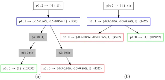
Example 4.4. Returning to Example 4.1, the computed Conley-Morse graph overQis indicated in Figure 4.3(a). The three Morse setsMQ(pi),i= 2,4,5, indicated by the shaded boxes have no nonzero eigenvalues. The numbers in parentheses indicate the number of boxes that define each combinatorial Morse setMQ(pi). Remark 2.3.2 raises the possibility – but does not imply – that MQ(pi) = ∅ for i = 2,4,5. This possibility is reinforced by the observation that there are very few boxes inMQ(pi) fori= 2,4,5.
To test whether the Morse sets with trivial index may, in fact, be numerical artifacts we need to be able to study them at a finer level of resolution.
4.4. Combinatorial Morse set refinement. Observe that ifMQ(p) is a com- binatorial Morse set determined by an outer approximationFQ(d), then the restriction FQ(d):MQ(p)−→→ MQ(p) is a closed graph. Choosed0 greater thand. DefineYQ(d0) to be the grid for|MQ(p)|, constructFQ(d0):YQ(d0)−→→ Y(d
0)
Q , and computeSQ(d0), the max- imal closed directed graph inFQ(d0). By Proposition 3.1 all the recurrent dynamics of
p0 : 2 {-1} (1)
p1 : 1 {-0.5-0.866i, -0.5+0.866i, 1} (1457)
p4 : 0 (11)
p2 : 0 (8)
p3 : 0 {-0.5-0.866i, -0.5+0.866i, 1} (4522) p6 : 0 {1} (105052)
p5 : 0 (4)
(a)
p0 : 2 {-1} (1)
p1 : 1 {-0.5-0.866i, -0.5+0.866i, 1} (1457)
p2 : 0 {-0.5-0.866i, -0.5+0.866i, 1} (4522) p3 : 0 {1} (105052)
(b)
Fig. 4.3. (a) The Conley-Morse graph computed over the parameter box Q defined by (q1, q2) = (20,33)andd`= 12. The three Morse sets indicated by the shaded boxes have no nonzero eigenvalues. (b) The trivially reduced Conley-Morse graph overQ.
MQ(p) is contained inSQ(d0), because MQ(p) = Inv |SQ(d0)|, FQ
= Inv |MQ(p)|, FQ
.
4.5. Conley-Morse graph reduction test. The first step is to apply theCom- binatorial Morse Set Refinement algorithm withd=d` andd0 =d`+ 1. There are two possible outcomes.
1. SQ(d0) = ∅. In this case MQ(p) = ∅, so we remove the vertex p and replace CMG(FQ(d`)) with its trivial reduction.
2. SQ(d0)6=∅. In this case there are two other options: Either we halt and accept CMG(FQ(d`)) as the appropriate Conley-Morse graph over Q, or we apply theCombinatorial Morse Set Refinement procedure to SQ(d0) and repeat the process.
In practice there are two constraints to this procedure. The first is the number of iterations before accepting that a Morse set with trivial index remains in the Conley- Morse graph. In the computations performed for this paper we stopped after three iterations. The second arises from memory considerations. If the combinatorial Morse set consists of a large number of boxes, then representing it on a finer grid can produce an impractically large set. In the computations performed for this paper we did not apply theCombinatorial Morse Set Refinementto sets consisting of more than 40,000 boxes.
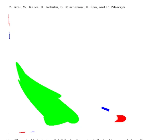
Example 4.5. Continuing with Example 4.4, after applying one iteration of the Conley-Morse Graph Reduction Test withd0 = 13 it is determined thatMQ(pk) =∅, for k = 2,4,5. This leads to the trivially reduced Conley-Morse graph indicated in Figure 4.3(b). The sets MQ(pk) for the reduced Conley-Morse graph over Q are indicated in Figure 4.4.
Recall that the desired database is a continuation graph. The first step is to create the continuation classes. Observe that over eachQ∈ Qwe have computed the trivially reduced Conley-Morse graphs CMG(FQ). We still retain the information of
Fig. 4.4. The sets MQ(pi), i = 0,1,2,3, for the reduced Conley-Morse graph from Fig- ure 4.3(b). The color coding in the two figures match, thus the green and red regions indicate attracting neighborhoods forfλfor allλin the parameter box Qdefined by(q1, q2) = (20,33)and d`= 12. The set MQ(p0)covers the origin and consists of a single box at the lower left corner of the picture and is barely visible at this resolution.
the boxes{MQ(p)|p∈ PQ}which define the vertices of CMG(FQ) and of course the ordering>Q between the vertices.
4.6. Continuation graph construction. LetQ0andQ1be grid elements such that Q0∩Q1 6= ∅. In order to determine whether CMG(FQ0) and CMG(FQ1) are equivalent, we proceed with the following steps:
1. If the cardinalities ofPQ0 and PQ1 differ then Q0 andQ1 do not belong to the same continuation class.
2. If the cardinalities of PQ0 and PQ1 agree, then we construct the clutching graph (see comment preceding Definition 3.5). If the clutching graph de- fines a directed graph isomorphism between the Morse graphs MG(FQ0) and MG(FQ1), then the Conley-Morse graphs CMG(FQ0) and CMG(FQ1) over Q0and Q1 belong to the same continuation class.
3. The clutching graph can fail to define a directed graph isomorphism between the Morse graphs MG(FQ0) and MG(FQ1) in several ways:
• The partial orders do not agree, in which case CMG(FQ0) and CMG(FQ1) are not identified as belonging to the same continuation class.
• There is a vertex with no edge in the clutching graph, in which case CMG(FQ0) and CMG(FQ1) do not belong to the same continuation class.

![Fig. 5.1. The continuation graph computed for the density dependent Leslie population model (1.3) with Λ = {θ = (θ 1 , θ 2 ) ∈ [8,37] × [3,50]}, and p = 0.7](https://thumb-ap.123doks.com/thumbv2/123deta/7603116.2538932/18.892.195.577.672.868/continuation-graph-computed-density-dependent-leslie-population-model.webp)
![Fig. 5.2. Continuation diagram computed for the two-dimensional Leslie population model with θ 1 ∈ [8,37], θ 2 ∈ [3, 50], p = 0.7](https://thumb-ap.123doks.com/thumbv2/123deta/7603116.2538932/19.892.219.551.199.536/fig-continuation-diagram-computed-dimensional-leslie-population-model.webp)
