DOI 10.1007/s00158-015-1246-8
RESEARCH PAPER
Analytical sensitivity in topology optimization for elastoplastic composites
Junji Kato1·Hiroya Hoshiba1·Shinsuke Takase1·Kenjiro Terada2·Takashi Kyoya1
Received: 15 April 2014 / Revised: 9 March 2015 / Accepted: 22 March 2015 / Published online: 15 May 2015
© Springer-Verlag Berlin Heidelberg 2015
Abstract The present study proposes a topology optimiza- tion of composites considering elastoplastic deformation to maximize the energy absorption capacity of a structure under a prescribed material volume. The concept of a so- calledmultiphase material optimization, which is originally defined for a continuous damage model, is extended to elastoplastic composites with appropriate regularization for material properties in order to regularize material parame- ters between two constituents. In this study, we formulate the analytical sensitivity for topology optimization con- sidering elastoplastic deformationand its path-dependency.
For optimization applying a gradient-based method, the accuracy of sensitivities iscritical to obtain a reliable opti- mization result. The proposed analytical sensitivity method
Junji Kato
[email protected] Hiroya Hoshiba
[email protected] Kenjiro Terada
[email protected] Takashi Kyoya
1 Mechanics of Materials Laboratory,
Tohoku University, 6-6, Aoba, Aramaki, Aoba-ku, SENDAI 980-8579, Japan
2 International Research Institute of Disaster Science, Tohoku University, 468-1, Aoba, Aramaki, Aoba-ku, SENDAI 980-0845, Japan
takes the derivative of the total stress which satisfies equi- librium equation instead of that of the incremental stress and does not need implicit sensitivity terms. It is verified that the proposed method can provide highly accurate sensitivity enough to obtain reliable optimization results by comparing with that evaluated from the finite difference approach.
Keywords Topology optimization·Analytical sensitivity analysis·Elastoplasticity·Composites·Plane stress condition
1 Introduction
Structural composites such as fiber-reinforced plastic, alloy and concrete have been developed in the expectation that they will perform various functions appropriate to vari- ous purposes and usages. One of the advantages of such composites from the mechanical viewpoint is that they enable us to control the mechanical behavior of composite materials by effectively combining materials with different characteristics. This makes it possible to obtain materials with intended mechanical characteristics appropriate for the environment or conditions in which the materials will be applied.
Today, structural design intended to maximize the mechanical characteristics (advantages) of materials consti- tuting each composite, taking into sufficient consideration their material nonlinearity, has increasingly been promoted.
Often seen are structures such as metallic vibration dampers using the plastic deformation performance of low-yield- point steel alloys, fiber-reinforced concrete that prevents brittle fractures, and hysteretic damping composite rubber, which are designed to have improved toughness or energy
absorption capacity based on their plasticity. Since design taking into consideration such complex mechanical behav- ior is extremely difficult, computer-based numerical exper- iments are employed to find an optimal structure that sat- isfies intended objectives or given conditions. Use of such numerical analysis techniques, however, is still not effec- tive in finding an optimal structure, and so trial-and-error calculations end up being used. It is therefore necessary to develop a method of structural optimization to improve the energy absorption capacity of a structure through effective use of the material nonlinearity of composites.
Meanwhile, most studies concerning structural optimiza- tion focus on problems relating exclusively to simple struc- tures composed of a single, linear elastic material, because studying complex structures raises high calculation costs and is associated with difficult theories. Studies on opti- mization considering the material nonlinearity of a single material have reported various findings under the theme of sensitivity analysis. Regarding plastic material models, Yuge and Kikuchi (1995), Schwarz and Ramm (2001), Maute et al. (1998) and Schwarz et al. (2001) address optimization focusing on continuum models while Choi and Santos (1987), and Ohsaki and Arora (1994) discuss optimization considering elastoplastic behavior in discrete structures such as a truss structure. Bugeda et al. (1999) study shape optimization focusing on continuum damage models.
As to the structural optimization of composites, many studies have addressed the problems of determining the optimal angle of fiber in a fiber-reinforced composite (Hammer1999) (Stegmann and Lund 2005) and of deter- mining the optimal layout of constituent materials (Gibian- sky and Sigmund2000) (Sigmund and Torquato1997), but they mostly focus on a linear elastic regime, as do the stud- ies focusing on a single material. Moreover, to the best of the present authors’ knowledge, few studies have been reported on a method of optimization which takes into consideration both composites and material nonlinearity. For example, Swan and Kosaka (1997) study topology optimization for elastoplastic materials using the classical Voigt-Reuss mix- ing rules, while Bogomolny and Amir (2012) consider the Drucker-Prager plastic model in studying topology opti- mization for steel-reinforced concrete. Studies by Kato et al.
(2009), Kato and Ramm (2013) and Amir (2013) seem to be the only reported cases that address optimization by employing continuum damage models to consider the material nonlinear behavior of composites.
The present study, therefore, discusses topology opti- mization, taking into consideration the elastoplastic defor- mation behavior of composites to determine their optimal material layout, as a way to improve the energy absorption capacity of a structure through effective use of the material nonlinearity of composites, as stated earlier.
In addressing optimization, the method of sensitivity analysis used to take account of the nonlinear behavior of a structure, and its accuracy, are important. Various stud- ies (e.g., Kleiber et al. (1997); Kleiber and Kowalczyk (1996); Ohsaki and Arora (1994); Schwarz and Ramm (2001); Maute et al. (1998); Schwarz et al. (2001); Zhang and Kiureghian (1993); Hisada (1995)) have reported find- ings regarding methods of deriving sensitivity relevant to plastic materials.
A challenge in dealing with plastic materials is that their stress-strain relations become undifferentiable when they reach their yield point or unloading point, making it diffi- cult to correctly evaluate their stress sensitivity (derivative of stress with respect to design variables) at those points.
Although Ohsaki and Arora (1994) study this problem in detail, they focus only on truss structures. It is therefore necessary equally to examine continuum structures. The studies/reports on sensitivity analysis above found condi- tions necessary to obtain high-accuracy sensitivity to be:
(i) using a consistent elastoplastic tangent modulus in the Euler-backward integration scheme (Zhang and Kiureghian 1993), and (ii) using a stress-integration method based on the return mapping algorithm and ensuring that the sensi- tivity conforming thereto is derived in sensitivity analysis (Hisada1995).
Against this background, the present study, based on the method of deriving stress sensitivity proposed by Hisada (1995), aims to formulate a new method of sen- sitivity derivation to maximize the energy absorption capacity of composites, which is set as the objective function, and to verify the accuracy of the sensitivity obtained.
The novelty of this study is that the proposed sensitiv- ity approach for topology optimization can provide accurate sensitivity “even without calculating the implicit deriva- tives with respect to design variables”. Thus, we conduct neither the analytical direct differentiation method nor ana- lytical adjoint method. Incidentally, Hisada’s sensitivity approach premises the calculation of implicit derivatives with respect to design variables. This is the difference from our approach.
Furthermore, we derive the proposed sensitivity method in detail assuming not only the general three dimensional problem but also a plane stress problem which is more cumbersome to handle. This contribution may help readers’
understanding and be useful in practice.
The elastoplastic material model used in the present study is the von Mises elastoplastic material model employ- ing the linear isotropic hardening law, and for its stress integration, a backward-Euler integration scheme based on the return mapping algorithm is employed in which a con- sistent tangent modulus is used. Details of these are not given here as they have been provided in many documents,
though some equations necessary to explain the sensitivity derivation method are presented in theAppendixat the end of this paper.
2 Definitions of design variables and regularization 2.1 Definitions of design variables
This section defines the design variables in topology opti- mization for composites. The proposed topology optimiza- tion is based on the concept of the Solid Isotropic Micro- structure with Penalization of intermediate densities, or SIMP approach (Zhou and Rozvany 1991), extended to apply to composites. This concept, illustrated in Fig.1, is intended to represent the optimal layout of a two-phase com- posite consisting of two solid phases. The SIMP approach, which assumes a porous body consisting of a single mate- rial, defines design variables as material densities set for each finite element. The present study, on the other hand, assuming a two-phase composite, replaces design variables with the volume fraction of the constituents. Therefore, for the jth of the elements discretized into N(number) finite elements, the design variablesj(j =1,2,· · ·, N )can be defined as follows:
sj = rj
r0
, 0≤sj ≤1. (1)
Here,rjrepresents the volume of phase-2 at thejth element andr0represents the volume of the element. This means that the elements are occupied by phase-1 whensj =0 and by phase 2 whensj =1. In the case of 0< s <1, elements of the two phases are mixed. Using these design variables, inci- dentally, optimization of a single material (porous material) can also be performed by replacing the material constant of phase-2 with that of solid material and setting 0 for the material constant of phase-1.
j
Fig. 1 Concept of two-phase material optimization
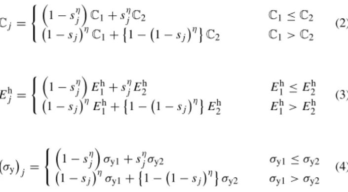
2.2 Regularization of elastoplastic material models In this study, composite material is simply modeled by the extended SIMP like approach. Here, the material parameters in the elastoplastic model are regularized with an interpo- lation scheme. AppendixAprovides three material param- eters of the elastoplastic model; elastic stiffness tensor C, work hardening modulusEhand initial yield stressσy. The present study sets these effective material parameters using the design variablesjas follows.
Cj = 1−sjη
C1+sjηC2 C1≤C2
1−sjη
C1+ 1−
1−sjη
C2 C1>C2
(2)
Ejh= 1−sjη
E1h+sjηE2h E1h≤E2h 1−sjη
E1h+ 1−
1−sjη
E2h E1h> E2h (3)
σy
j= 1−sηj
σy1+sjησy2 σy1≤σy2
1−sjη
σy1+ 1−
1−sjη
σy2 σy1> σy2
(4)
where η is an exponential parameter. As shown above, the parameters of two materials are interpolated in smooth functions. This is called regularization. These equations are obtained by applying to plastic material a regulariza- tion method for two-phase material optimization based on the damage model of the present authors and others (Kato et al. 2009). This makes the material parameters of each element dependent on design variables, meaning that the design variables that control the topology of a structure are embedded.
3 Setting the optimization problem
The present study sets the energy absorption capacity of a composite structure subject to plastic deformation as the objective function and aims to maximize it. Absorbed energy can be expressed as the total work for displace- ment of the control point, and the work can be measured by the area bounded by the load-displacement curve. The con- straint is that the volume of the material used in the entire structure should be constant. The objective functionf (s) and the equality constanth (s)are set as follows:
minimize f (s) = −
t 0
σ : ˙εdtd
= −
εˆ
σ :dεd, (5)
subject to h (s)=
sjd− ˆV =0, (6)
where,σ andεrepresent the Cauchy stress tensor and the linear strain tensor, respectively.tand (˙•) represent time and the time derivative, respectively.εˆis the total strain follow- ing the control point displacementu,ˆ Vˆ is the volume of phase-2 in the entire structure, andsis the design variable (vector) expressed bys= {s1,· · ·, sN}.
Note that the objective function above is multiplied by - 1 to form a minimization problem because an optimization problem is generally set as a minimization problem. The present optimization problem is solved by employing the optimality criteria (Patnaik et al.1995).
4 Derivation of sensitivity
4.1 Derivation of sensitivity of the objective function This section proposes a method of deriving formulae to eval- uate the sensitivity of the objective function. The present study, to solve this nonlinear structural problem quasi- statically, replaces (5) with the incremental one shown below, using the pseudo-time (or load step) variablenstep, f (s)=
nstep
n=1
fn(s) , (7)
where, nstep represents the total number of load steps.
fn indicates the value of the objective function obtained between timen−1 and timen, and can be expressed as follows:
fn(s)= −
σn :dεnd. (8)
Based on the above, the gradient of the objective func- tion with respect to a specific design variablesj is obtained.
For the sake of simplicity, ∂s∂
j shall hereafter be expressed as
∇sj
. First, the gradient of (7) can be calculated as follows:
∇sjf (s)=
nstep
n=1
∇sjfn(s) . (9)
For the gradient of (8), to ensure consistency with subse- quent explanations, the equation below describes the objec- tive function valuefn+1obtained between time nand the current timen+1,
∇sjfn+1 = −∇sj
⎛
⎝
σn+1:dεn+1d
⎞
⎠
= −
∇sjσn+1
:dεn+1+σn+1: ∇sjdεn+1 d.(10)
Note that this paper assumes that the variables at time nare already known. Since the strain increment dεn+1is a variable obtained through structural analysis of the current timen+1, its gradient∇sjdεn+1cannot be derived explic- itly. Therefore, ∇sjdεn+1 is called the implicit derivative term. The present study first eliminates this∇sjdεn+1under the conditions below.
The weak form of the equilibrium equation at timen+1, namely, the equation of the principle of virtual work, is as follows:
σn+1:δεd−λn+1 t
t0·δud t=0. (11) Here,λn+1indicates the load factor at the current time andt0is the reference traction force vector, which is a con- stant value. Body force is neglected in this study for the sake of simplicity, without loss of generality of the equa- tion of equilibrium. Next, since virtual displacementδuand its corresponding virtual strain δε can be arbitrarily cho- sen in an equation of virtual work, replacing them with δε= ∇sjdεn+1andδu= ∇sjdun+1in (11) can still satisfy the equilibrium,
σn+1: ∇sjdεn+1d−λn+1
t
t0· ∇sjdun+1d t=0. (12) The gradient here is not related to the design variable vectorsbut tosj, a component of the design variable, and therefore∇sjdεn+1(or∇sjdun+1) is a tensor of the same dimension as virtual strain (or virtual displacement). As a result, there is no dimensional inconsistency, mathemati- cally, in (12).
After presenting these equations, the present study assumes a special load condition whereby load affects the displacement control nodes alone. First, since the dis- placement element uˆ or its increment duˆ applied to the displacement control node is determined as a load condition regardless of the design variables, its gradient is expressed as∇sjduˆ = 0. Considering also that the reference traction force vectort0is always constant and does not depend on the design variables, the displacement increment vector for the entire control node dun+1(of duˆn+1) can be identified ast0·∇sjdun+1=0. This is the integrand of the second left- hand term of (12). Thus, (12) can be simplified as follows,
σn+1: ∇sjdεn+1d=0. (13) As a result, under this load condition, the second term of (10) can be eliminated and (10) can be rewritten as follows,
∇sjfn+1= −
∇sjσn+1
:dεn+1d. (14)
With this, the sensitivity of the objective function can be obtained by identifying the gradient of stress with respect to the design variable∇sjσn+1. Hereafter, ∇sjσ shall be called stress sensitivity.
Meanwhile, Maute et al. (1998), Schwarz et al. (2001), and Schwarz and Ramm (2001) also address optimization problems setting maximization of energy absorption capac- ity as the objective function. To derive sensitivity, they first define the stress increment dσn+1as:
dσn+1=Cep∗:dεn+1, (15)
and start by directly differentiating the stress sensitivity as follows,
∇sjdσn+1= ∇sjCep∗:dεn+1+Cep∗: ∇sjdεn+1. (16) Here,Cep∗represents the consistent tangent modulus tensor.
Next, they substitute (16) into (10), add (9) and rearrange as follows:
∇sjf = −
εˆ ε
dε: ∇sjCep∗:dε
+2 dε:Cep∗: ∇sjdε
d. (17)
Moreover, as mentioned earlier, they eliminate implicit terms by setting a special load condition, so as to propose an equation to evaluate sensitivity of the objective function as shown below,
∇sjf = −
εˆ ε
dε: ∇sjCep∗:dεd. (18) This equation enables us to obtain sensitivity of the objective function merely by identifying the gradient of the tangent modulus tensor∇sjCep∗. It should be noted, though, that (15), which is the starting point of these processes, is formulated to identify the equilibrium point in structural analysis and therefore it may not express the stress incre- ment correctly. In short, the equation for stress sensitivity presented by Maute et al. (1998), Schwarz et al. (2001), and Schwarz and Ramm (2001) does not aim at the sensitiv- ity of stress that satisfies equilibrium equation. This results in an accumulation of errors in stress sensitivity as plas- tic deformation progresses, with particularly large errors at yield points and the points at which stress changes due to unloading, etc., or, in other words, in the vicinity of undifferentiable points.
In other words and strictly speaking, the stress increment dσn+1or the stressσn+1(=σn+Cep∗ : dεn+1)obtained from (15) don’t satisfy the equilibrium equation although they satisfy the tolerance of convergence of equilibrium equation. The final stress which satisfies the equilibrium equation, denoted asσ(F)n+1later, is calculated after determin- ing equilibrium point, using obtained nodal displacement through (22) based on the return mapping algorithm, see
Section4.3. In that sense, the incremental stress dσn+1or the consistent tangent operatorCep∗are simply employed as a “tool” to determine/identify the equilibrium point.
Thus, to ensure the accuracy of the sensitivity evalua- tion (14), the present study aims to identify the sensitivity
∇sjσ(F)n+1 of the stress that satisfies the equilibrium equa- tion. To summarize, we should directly take a derivative of σ(F)n+1 with respect to a design variable rather than that of σn+1and replace∇sjσn+1in (14) by∇sjσ(F)n+1.
In this derivation procedure, details of which are pro- vided in Section 4.3, ∇sjσ(F) shall be updated taking into consideration the path-dependency in each incremental step. The procedures for conditional differentiation and for obtaining stress sensitivity described below are formulated referring to the work of Hisada (1995).
4.2 Conditional differentiation
This section outlines the concept of conditional differenti- ation, which is employed in the following section. In con- ducting optimization using an elastoplastic material model and incremental analysis, stressσ, for example, can be con- sidered as a function composed of displacementu(s)and design variables. Therefore,σn+1at the current timen+1 can be expressed as
σn+1 =σn+1(un+1(s) ,un(s) ,un−1(s) ,· · ·,
u1(s) ,s) . (19)
This equation shows that the objective function in thenth step is determined not only by un+1 but also by the past history. With regard to the calculus used to solve such path- dependent problems, the variation of (19) resulting from the variationδsjof design variables is as follows:
δσn+1= ∂σn+1
∂un+1
δun+1+δ∗σn+1, (20) where,
δ∗σn+1 ≡ ∂σn+1
∂un
δun+∂σn+1
∂un−1
δun−1
+· · · +∂σn+1
∂u1
δu1+∂σn+1
∂sj
δsj
≡ d∗σn+1
dsj
δsj. (21)
δ∗σn+1 fixes onlyun+1 and represents the variation (con- ditional variation) of σn+1 taking into consideration the variations of all other variables, and d∗σn+1/dsj similarly represents conditional variation. For the sake of simplicity, d∗/dsjshall be expressed as∇s∗j hereafter.
4.3 Derivation of stress sensitivity
This section explains the procedure used to obtain the stress sensitivity∇s∗jσn+1at the current timen+1, assuming an increment from timento the current timen+1, using the values known at time n. In this procedure, the stress sensitiv- ity and the gradient of relevant values with respect to design variables are used as the known values for the subsequent incremental step, which enables updating of stress sensitiv- ity taking into consideration the history up to then. Here, the conditional differentiation explained above is used to obtain gradients with respect to design variables, and gradients are all set at zero initially. Details of each of the variables presented in this section are provided in theAppendixfor reference.
First, the final stress at the current timen+1 is decom- posed into the deviatoric and volumetric parts,
σ(F)n+1=σ(F)n+1+p(F)n+1:I. (22) Then partially differentiating both sides gives the following:
∇s∗jσ(F)n+1= ∇s∗jσ(F)n+1+ ∇s∗jp(F)n+1:I, (23) where,pandIare hydrostatic pressure and 2nd-order iden- tity tensor, respectively. The two derivative terms on the right-hand side of (23) are derived separately as follows.
First, we refer to some equations listed in theAppendixto obtain∇s∗jσ(F)n+1.
From (62), the plastic multiplier is rewritten by substitut- ing the final equivalent stressσ¯n(F)+1,
γ =3 2
ε¯p
¯
σn(F)+1, (24)
and substituting this into (68) yields a relation of the trial and final stresses as follows:
σ(F)n+1= 1
1+2Gγσ(T)n+1. (25)
Here, partially differentiating (25) with∇s∗j yields:
∇s∗jσ(F)n+1= ∇s∗jσ(T)n+1
1+2Gγ−2G∇s∗j(γ )+2γ∇sjG
(1+2Gγ )2 σ(T)n+1. (26) This indicates that∇s∗jσ(T)n+1,∇s∗j(γ ), and∇s∗jGneed to be obtained.∇s∗jGcan be easily identified because it is a component of the elastic modulus tensor of (2). As for
∇s∗j(γ ), conducting partial differentiation of (24) with∇s∗j
yields
∇s∗j(γ )= 3 2
⎛
⎜⎝∇s∗j(ε¯p)
¯
σn(F)+1 −ε¯p∇s∗jσ¯n(F)+1 σ¯n(F)+12
⎞
⎟⎠, (27)
where∇s∗j(ε¯p)and∇s∗jσ¯n(F)+1 are needed. Therefore, the following shows how to identify the three derivative terms including ∇s∗j(ε¯p) and ∇s∗jσ¯n(F)+1, as well as ∇s∗jσ(T)n+1 mentioned above.
First, in accordance with the return mapping algorithm, we introduce basic equations concerning trial stress and final stress. Using (64), deviatoric stress can be expressed as follows:
σ(T)n+1=σn+2Gε. (28) Using equation (59), an equation to express trial stress can be obtained as follows:
σ¯ (T)n+12
= 3 2
σ(T)n+1:σ(T)n+1
. (29)
Taking into account its dependence on design variables, (71) is rewritten as follows:
¯
σn(F)+1=k
¯ εpn+1,s
. (30)
Based on (70), the relation below for trial stress and final stress can be obtained,
¯
σn(F)+1= ¯σn(T)+1−3Gε¯p. (31) Then partially differentiating these (28) – (31) yields the following equations, in order,
∇s∗jσ(T)n+1= ∇s∗jσn+2
∇sjG
ε, (32)
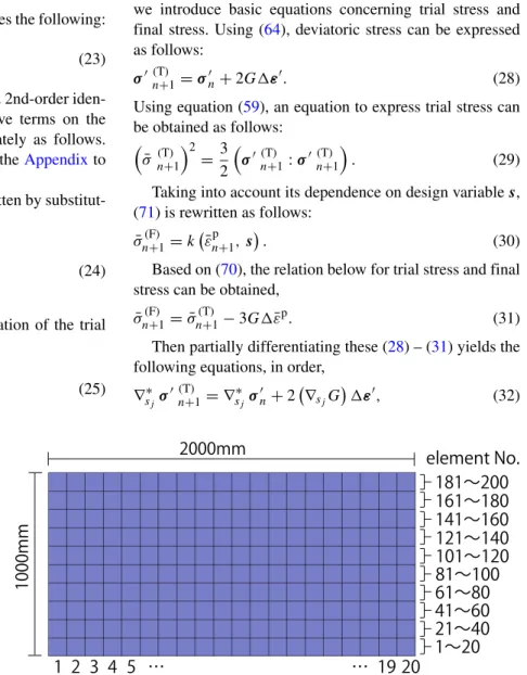
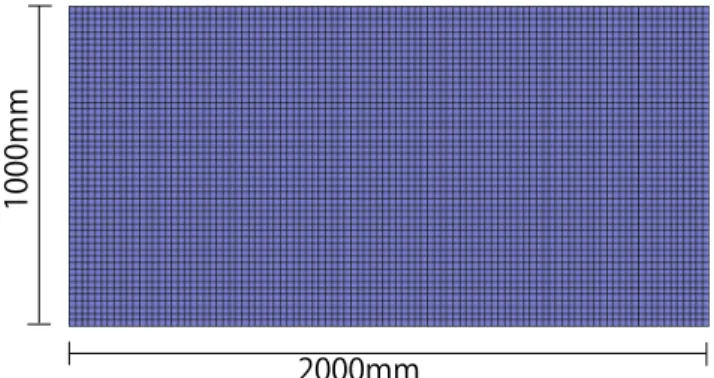
Fig. 2 Finite element mesh used for verification of sensitivity
1000mm
2000mm
1〜20 21〜40 41〜60 181〜200 161〜180
1 2 3 4 5 20
141〜160 121〜140 61〜80 81〜100 101〜120 element No.
… … 19
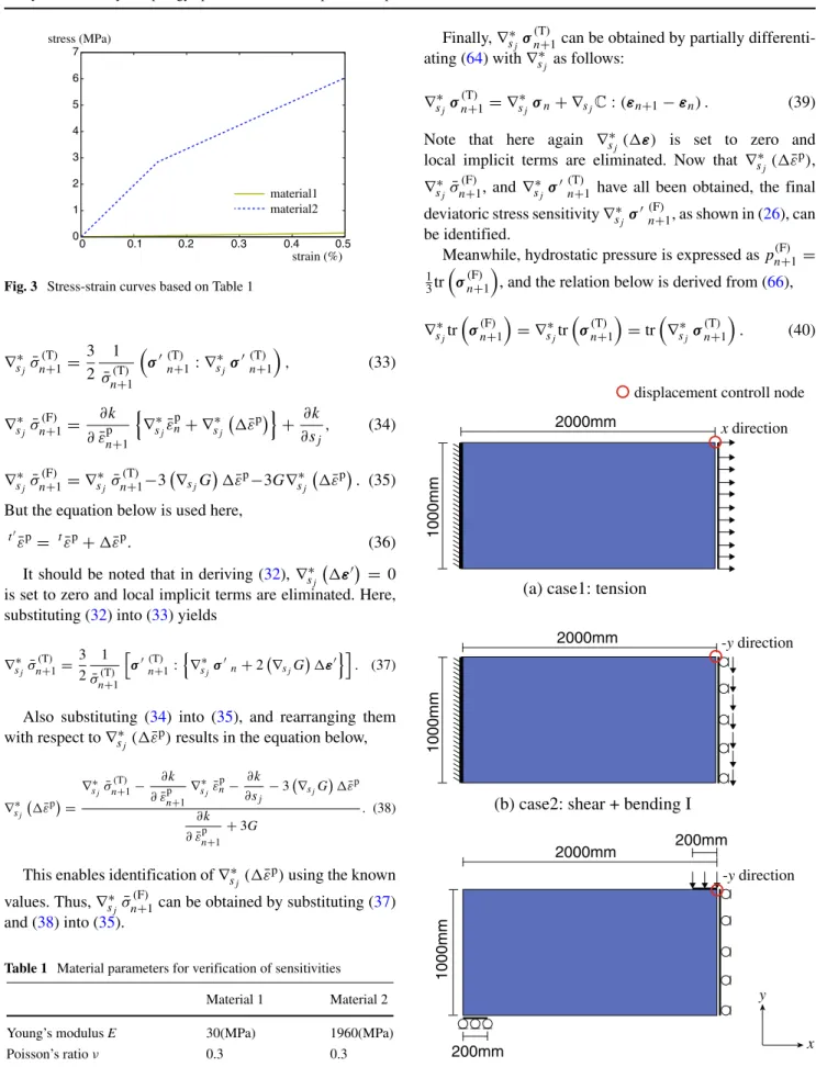
0 1 2 3 4 5 6 7
0 0.1 0.2 0.3 0.4 0.5
stress (MPa)
strain (%) material1 material2
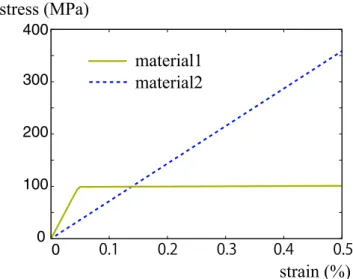
Fig. 3 Stress-strain curves based on Table 1
∇s∗jσ¯n(T)+1= 3 2
1
¯ σn(T)+1
σ(T)n+1: ∇s∗jσ(T)n+1
, (33)
∇s∗jσ¯n(F)+1= ∂k
∂ε¯np+1
∇s∗jε¯np+ ∇s∗j
ε¯p + ∂k
∂sj
, (34)
∇s∗jσ¯n(F)+1= ∇s∗jσ¯n(T)+1−3
∇sjG
ε¯p−3G∇s∗j
ε¯p . (35) But the equation below is used here,
tε¯p= tε¯p+ε¯p. (36)
It should be noted that in deriving (32),∇s∗j
ε
= 0 is set to zero and local implicit terms are eliminated. Here, substituting (32) into (33) yields
∇s∗jσ¯n(T)+1=3 2
1
¯ σn+1(T)
σ(T)n+1:
∇s∗jσn+2
∇sjG ε
. (37)
Also substituting (34) into (35), and rearranging them with respect to∇s∗j(ε¯p)results in the equation below,
∇s∗j ε¯p
=
∇s∗jσ¯n+1(T) − ∂k
∂ε¯n+1p ∇s∗jε¯np− ∂k
∂sj −3
∇sjG ε¯p
∂k
∂ε¯n+1p +3G
. (38)
This enables identification of∇s∗j(ε¯p)using the known values. Thus,∇s∗jσ¯n(F)+1can be obtained by substituting (37) and (38) into (35).
Table 1 Material parameters for verification of sensitivities Material 1 Material 2
Young’s modulusE 30(MPa) 1960(MPa)
Poisson’s ratioν 0.3 0.3
initial yielding stressσy 1.0(MPa) 2.9(MPa)
hardening modulusEh 10(MPa) 900(MPa)
Finally,∇s∗jσ(T)n+1can be obtained by partially differenti- ating (64) with∇s∗j as follows:
∇s∗jσ(T)n+1= ∇s∗jσn+ ∇sjC:(εn+1−εn) . (39) Note that here again ∇s∗j(ε) is set to zero and local implicit terms are eliminated. Now that ∇s∗j(ε¯p),
∇s∗jσ¯n(F)+1, and∇s∗jσ(T)n+1 have all been obtained, the final deviatoric stress sensitivity∇s∗jσ(F)n+1, as shown in (26), can be identified.
Meanwhile, hydrostatic pressure is expressed asp(F)n+1=
1 3tr
σ(F)n+1
, and the relation below is derived from (66),
∇s∗jtr
σ(F)n+1
= ∇s∗jtr
σ(T)n+1
=tr
∇s∗jσ(T)n+1
. (40)
1000mm
2000mm x direction
1000mm
2000mm
1000mm
200mm
200mm (a) case1: tension
(b) case2: shear + bending I
(c) case3: shear + bending II
x y 2000mm -y direction
-y direction displacement controll node
Fig. 4 Boundary conditions
-12000 -10000 -8000 -6000
0 40 80 120 160 200
element No.
finite difference method analytical method
sj
f
Fig. 5 Accuracy of sensitivities for case1 (tension)
Based on this, the sensitivity of hydrostatic pressure can be expressed as follows:
∇s∗jpn(F)+1=1 3tr
∇s∗jσ(T)n+1
. (41)
By substituting (39) into this equation, the sensitivity1 of hydrostatic pressure can be obtained.
Thus, the final stress sensitivity∇s∗jσ(F)n+1can be obtained by substituting∇s∗jσ(F)n+1and∇s∗jpn(F)+1identified here into (23). And by using this in (14), the sensitivity of the objec- tive function which is consistent with the stress that satisfies the equilibrium equation obtained by implicit integration, can be obtained.
4.4 Stress sensitivity for plane stress condition
In the previous section, derivation of stress sensitivity assuming a return mapping algorithm for a general three
-8000 -6000 -4000 -2000 0
0 40 80 120 160 200
element No.
finite difference method analytical method
sj
f
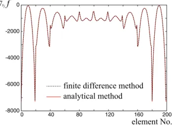
Fig. 6 Accuracy of sensitivities for case2 (shear+bending I)
-6000 -4000 -2000 0
0 40 80 120 160 200
element No.
finite difference method analytical method
sj
f
Fig. 7 Accuracy of sensitivities for case3 (shear+bending II)
dimensional problem was presented. In this section, we for- mulate it assuming a plane stress problem, which is a little bit troublesome to handle but is useful in practice. The expression of a return mapping algorithm for plane stress problem is referred to AppendixB(B2), which is based on Simo and Huches (1998).
First of all, we take a derivative of (77) with respect to a design variable utilizing a conditional derivative ∇s∗j as follows:
1
2∇s∗jξ−2 3k·
∂k
∂ε¯pn+1∇s∗jε¯pn+1+ ∂k
∂sj
=0. (42)
Here, ∇s∗jξ and ∇s∗jε¯np+1 can be obtained by taking a conditional derivative of (83) and (78), respectively,
0 1 2 3 4 5 6
0 20 40 60 80 100 120 140 160
yielding
displacement of control node 1 mm
(elastic)
50 mm 100 mm
150 mm
(mm) (N)
Fig. 8 Load–displacement curve of case 1 showing the degree of underlying displacements of control node
-600 -550 -500 -450 -400 -350
0 40 80 120 160 200
element No.
finite difference method analytical method
sj
f
Fig. 9 Accuracy of sensitivities for case 4 (initial design variable 0.1)
∇s∗jξ =
σ11(T)+σ22(T) ∇∗sjσ11(T)+ ∇s∗jσ22(T) 3 [1+Eγ /{3(1−ν)}]2
−
σ11(T)+σ22(T) 2
∇s∗jE
γ+E∇s∗j(γ ) 9(1−ν)[1+Eγ /{3(1−ν)}]3
+
σ22(T)−σ11(T) ∇s∗jσ22(T)− ∇∗sjσ11(T) +4σ12(T)
∇s∗jσ12(T) (1+2Gγ )2
− 2
σ22(T)−σ11(T) 2
+4
σ12(T) 2
∇s∗jG
γ+G∇s∗j(γ )
(1+2Gγ )3 (43)
∇s∗jε¯pn+1= ∇s∗jε¯pn+ 2
3
⎧⎨
⎩∇s∗j(γ )
ξ+γ
∇∗sjξ 2√
ξ
⎫⎬
⎭. (44)
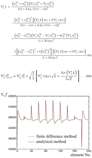
-40000 -36000 -32000 -28000 -24000 -20000
0 40 80 120 160 200
element No.
finite difference method analytical method
sj
f
Fig. 10 Accuracy of sensitivities for case 4 (initial design variable 0.9)
Next, a derivative of the trial stress ∇s∗jσˆn(T)+1 shown in AppendixBcan be written by eliminating the local implicit derivative term, namely to be∇s∗j
εˆ
=0, as follows:
∇s∗jσˆn(T)+1= ∇s∗jσˆn+
∇s∗jC
ε.ˆ (45)
As can be seen, (45) consists of the explicit derivative terms only. Thus, (42) together with (43), (44) can be solved simultaneously for the unknown∇s∗j(γ ).
Furthermore, taking a conditional derivative of (74), (84), (85) yields,
∇s∗jσˆn(F)+1=
∇s∗jA
σˆn(T)+1+A
∇s∗jσˆn(T)+1
(46) where
∇∗sjA=
⎡
⎢⎢
⎣ 1 2
∇s∗jA∗11+ ∇s∗jA∗22 1
2
∇s∗jA∗11− ∇s∗jA∗22
0 1
2
∇s∗jA∗11− ∇s∗jA∗22 1
2
∇s∗jA∗11+ ∇s∗jA∗22
0
0 0 ∇s∗jA∗33
⎤
⎥⎥
⎦ (47)
and
∇s∗jA∗11 = −3(1−ν)
∇s∗jE
γ+E∇s∗j(γ ) {3(1−ν)+Eγ}2 ,
∇s∗jA∗22 = −2
∇s∗jG
γ+G∇s∗j(γ )
(1+2Gγ )2 ,
∇s∗jA∗33 = ∇s∗jA∗22. (48) Finally, the stress sensitivity of the final stress ∇s∗jσˆn(F)+1 can be obtained by substituting∇s∗j(γ )into (46)–(48).
-600 -500 -400 -300
0 40 80 120 160 200
element No.
finite difference method analytical method
sj
f
Fig. 11 Accuracy of sensitivities for case 5;uˆ=1mm (elastic range)
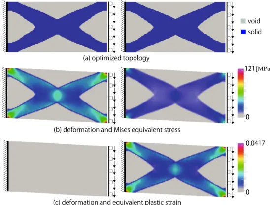
![Fig. 15 Optimization results for case 1 (tension): (left) elastic, (right) plastic 0 0.04170100.2 [MPa]01000.solidvoid(a) optimized topology (c) deformation and equivalent plastic strain(b) deformation and Mises equivalent stress](https://thumb-ap.123doks.com/thumbv2/123deta/7351074.2437032/11.892.346.813.91.424/optimization-solidvoid-optimized-topology-deformation-equivalent-deformation-equivalent.webp)