Chapter 3
The Feasibility Study of the Dynamic Zone Configuration Technique with a Developed Circular Array Antenna
3.1 Introduction
The growing demand for wireless mobile communication is putting increasing strains on the frequency spectrum, a finite and scarce resource. To cope with this situation, the techniques for more effectively utilizing the radio spectrum must be developed. The dynamic zone configuration (DZC) technique, which uses array antenna at base station (BS) and controls the zone shape according to mobile stations’ (MSs’) distribution adaptively, is a promising approach to improve the spectrum efficiency.
The DZC technique provides several merits to all temporal access schemes for wireless communication systems, such as “frequency division multiple access (FDMA)”, “time division multiple access (TDMA)”, and “code division multiple access (CDMA)”. It reduces co-channel interference and multipath fading, because the DZC directs the antenna beam pattern toward the desired area. As a result, it reduces the outage probability and increases the capacity and quality of service (QoS) [1].
However, in order to realize such wireless communication systems with DZC technique, the types of antenna used at BS and the algorithm used to form the beam based on the distribution of MSs are the most important issues to discuss. The current consensus is that DZC can best be achieved by using the array antenna or the sectorized antenna. For instance, [2] proposed a beam formation algorithm with 4-sectorized antenna, which controls dynamically the shapes of the zones by changing the radius of the zones and the beam width
The sectorized antenna is better from the viewpoint of controlling the zone shape, while the array antenna is better for achieving a precise zone shape configuration. However, with an array antenna, it is complicated to determine the optimum weight vector for each array element dynamically, which must be done to control the antenna gain to match the distribution of MSs. Moreover, from the viewpoint of signal processing, there is a trade-off between the tracking speed and accuracy of the shaped zone. This trade-off demands simple and fast-tracking algorithms, that can determine the weight vectors needed to shape the required zones.
In this chapter, the author newly proposes a simple tracking algorithm for reducing the complexities to determine the weight vector of each array element. In the proposed algorithm, firstly, BS categorizes the MSs into several groups in accordance with the distribution of MSs.
Then, from several information contained in each group such as width and direction of each group and so on, we decide the simple input parameters for the calculation method to determine the optimum weight vector for each array antenna. After that, using the simple input parameters, BS calculates the optimum weight vector and configures the required zone.
In this chapter, we introduce the “grouping algorithm” which categorizes the MSs into several groups and the “parameter setting method” which converts the several parameters related to the shape of each group into the input parameters for the calculation method of optimum weight vector. Then we evaluate the system performance such as call blocking rate (BR) and so on by introducing the DZC technique which utilizes the proposed method and algorithm to FDMA- FDD (frequency division duplex) system.
In addition to the proposal of simple DZC technique, in order to increase the system capacity, we investigate the effectiveness of combination between DZC and dynamic channel assignment (DCA) strategy, which improves frequency utilization efficiency. We also evaluate the system performance under the same FDMA-FDD based wireless communication
environment. In DCA, BS assigns traffic channels dynamically over cells according to the channel demands of each cell. A number of studies have been carried out this strategy and verified its effectiveness [4][5]. However, most papers do not mention the effectiveness of the combination.
Moreover, in order to show realistic feasibility, we utilize the measured characteristics of the developed circular 8-element array antenna [6] to evaluate the performance of the simulation.
This chapter is organized as follows: Section 3.2 describes the preposition with the 8-element array antenna we developed. Section 3.3 explains the simplified method we used to configure the zones. Section 3.4 presents the simulation results. Section 3.5 concludes with summary and a mention of further work.
3.2 Presupposition Condition in Calculation
The newly proposed DZC technique can be utilized for all of the array antenna systems if the author has only to know the basic characteristics of each array element such as the steering vector s(φ), which is the array response vector of each antenna element toward the direction φ (degree) in advance, and fix the calculation method to determine the optimum weight vector, which is the value of amplitude and phase given to each array element to radiate the radio signal toward the required direction. In this chapter, in order to evaluate the system performance using the proposed DZC technique actually, the author utilizes the characteristics of the array antenna prototype. In this section, the author explains the overview of the prototype, illustrates the basic antenna characteristics, and summarizes the calculation method to determine optimum weight vector, which is utilized in this prototype
3.2.1 Overview of the Developed Prototype
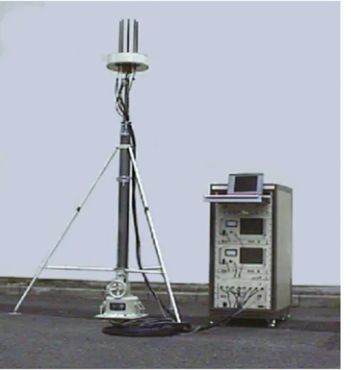
Figure 3.1(a) shows the developed adaptive zone configuration system prototype, which consists of a 2.335 GHz radio-frequency generator, a directivity controller to control the amplitude and phase components of the array antenna, and a circular, 8-element array antenna in which the antenna elements are arranged at equal-angle intervals [6]. Each array element is a dipole antenna and the length between each element is λ/2 as shown in Fig. 3.1(b). The transmission power is 10 W at vertical polarization. The steering vector of this antenna
( ) [ ( ), , ( )] | , , , , }
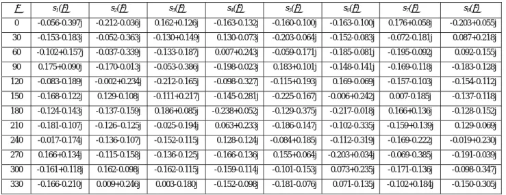
{sφ = s1φ smφ T φ=03060 330 is indicated in Table 3.1, where m is the number of elements and m =8 in this chapter. Superscript T denotes the transposition of matrix. In order to radiate the radio signal toward the required directions, the weight vector
[ 1, , ] ,( =8),
= w wm T m
w must be determined to each array element. In this experiment, the least square (LS) method was adopted. The next subsection describes the LS method theoretically.
(a) The photograph (b) 8-element array Fig 3.1. The overview of the developed prototype.
#5
#2
#3
#4
#6
#7
#8
#1 d
mπ/4
λ/2
Table 3.1. Steering vector s(φ).
φ s1(φ) s2(φ) s3(φ) s4(φ) s5(φ) s6(φ) s7(φ) s8(φ) 0 -0.056-0.397j -0.212-0.036j 0.162+0.126j -0.163-0.132j -0.160-0.100j -0.163-0.100j 0.176+0.058j -0.203+0.055j 30 -0.153-0.183j -0.052-0.363j -0.130+0.149j 0.130-0.073j -0.203-0.064j -0.152-0.083j -0.072-0.181j 0.087+0.218j 60 -0.102+0.157j -0.037-0.339j -0.133-0.187j 0.007+0.243j -0.059-0.171j -0.185-0.081j -0.195-0.092j 0.092-0.155j 90 0.175+0.090j -0.170-0.013j -0.053-0.386j -0.198-0.023j 0.183+0.101j -0.148-0.141j -0.169-0.118j -0.183-0.128j 120 -0.083-0.189j -0.002+0.234j -0.212-0.165j -0.098-0.327j -0.115+0.193j 0.169-0.069j -0.157-0.103j -0.154-0.112j 150 -0.168-0.122j 0.129-0.108j -0.111+0.217j -0.145-0.281j -0.225-0.167j -0.006+0.242j 0.007-0.185j -0.137-0.118j 180 -0.124-0.143j -0.137-0.159j 0.186+0.085j -0.238+0.052j -0.129-0.375j -0.217-0.018j 0.166+0.136j -0.128-0.152j 210 -0.181-0.107j -0.126–0.125j -0.025-0.194j 0.063+0.233j -0.186-0.147j -0.102-0.335j -0.159+0.139j 0.129-0.069j 240 -0.017-0.174j -0.136-0.107j -0.152-0.115j 0.128-0.124j -0.084+0.185j -0.112-0.319j -0.169-0.222j -0.019+0.230j 270 0.166+0.134j -0.115-0.158j -0.136-0.125j -0.166-0.136j 0.155+0.064j -0.203+0.034j -0.069-0.385j -0.191-0.039j 300 -0.161+0.118j 0.162-0.098j -0.162-0.115j -0.159-0.114j -0.101-0.153j 0.073+0.235j -0.171-0.136j -0.098-0.347j 330 -0.166-0.210j 0.009+0.246j 0.003-0.180j -0.152-0.098j -0.181-0.076j 0.071-0.135j -0.102+0.184j -0.150-0.305j
3.2.2 A Method for Providing Optimum Weight Vector
In the DZC system, in order to radiate the radio signal toward the desired direction, the optimum weight vector must be determined for each antenna element. A lot of algorithms have been proposed for providing the optimum weight vector [7][8]. The least square (LS) method [7] is adopted. According to this method, first of all, the desired directions θj (j = 1 Nd), the required antenna gain gj (j = 1 Nd) toward θj, and the undesired directions ψk (k = 1 ,Nu) are determined, where Nd and Nu are the number of desired directions and undesired directions, respectively. The values of Nd and Nu depend on the MSs’ distribution. Here, the undesired direction means the direction that should be suppress the radiation, not the direction of arrival of undesired wave. Then, by using these parameters and steering vector s(φ),the optimum weight vector which minimizes a cost function J is obtained as shown in following equation:
2 2
1 1
( ) ( )
d u
N N
T T H
j j k
j k
θ g α ψ β
= =
=
∑
− +∑
+J w s w s w w (3.1)
second term is the square value of the gain in the undesired directions, and the third term is for minimizing the output power. In eq. (3.1), α and β are the weight coefficients for minimizing the radiation in the undesired directions and the total radiation (0≤α, 0<β), respectively. H denotes Hermitian transposition (i.e., transposition combined with complex conjugation).
In order to minimize the cost function in eq. (3.1), the author applies the gradient operator
) ( ] , , ,
[∇ 1 ∇ 2 ∇ =8
=
∇w w w wm T m to the cost function J. The gradient operation is given as follows:
1 2
1 2
[ , , , ] , , , .
T T
m
w w wm
⎡ ∂ ∂ ∂ ⎤
∇w = ∇w ∇w ∇w = ⎢⎣∂ ∂ ∂ ⎥⎦
J J J
J J J J (3.2)
The optimum weight vector wopt satisfies the following condition:
∇wJ=0 . (3.3) By solving eq. (3.3), wopt is given by
1 opt
= −
w R r, (3.4) where
* *
1 1
( ) ( ) ( ) ( ) ,
d u
N N
T T
j j k k
j k
θ θ α ψ ψ β
= =
=
∑
+∑
+R s s s s I (3.5)
* 1
( ) .
Nd
j j
j
θ g
=
=
∑
r s (3.6)
The asterisk ‘*’ denotes complex conjugation and I is the m- by-m identity matrix.
In order to investigate the effectiveness of the above method, the author compared the simulation result obtained from eq. (3.4) and s(φ) shown in Table 3.1 with the experimental result from the prototype [9]. In the simulation result, the example parameters and calculated the weight vector wopt from eq. (3.4) are assumed. Here, 0o is set to be a point due east, with
angles increasing in the counterclockwise direction. The the following parameters are set.
Nd =2, θ [degree] = [324, 351], g = [1, 1],
Nu =10, ψ [degree]= [50, 66.25, 82.5, 98.75, 115, 197, 209, 221, 234, 245], α =0.1, β =0.1,
where
θ = [θ 1 … θ Nd], g = [ g1 … g Nd], ψ = [ψ 1 … ψNu].
To sample the experimental data, the prototype was mounted on a 60 m high tower and was inputed the weight vector wopt for the prototype. A mobile measurement vehicle drove around the tower, receiving the signals transmitted from the BS. This vehicle took measurements every 4 mm. Using this sampled data, the medium value was calculated every 1 m. Figure 3.2 shows the comparison results. Figure 3.2(a) represents the calculated zone shape by computer simulation, while Fig. 3.2(b) shows the measured zone shape. The received levels shown in this figure is the relative ratio to the received level of an omni-directional zone. These results show that the simulation environment is quite close to the real prototype environment.
-10 0 10
-10 0 10
N
S
W E
N
W
S
E
[dB] [dB]
(a) Calculation result (b) Measurement result
3.3. Simplified Method for Dynamic Zone Configuration
3.3.1. Problems in Conventional Dynamic Zone Configuration Technique
In this subsection, by utilizing a example of array antenna described in the above section, the author clarify a important problem of the conventional DZC technique. In the example of the previous section, a circular 8-element array antenna was introduced. In theoretically, if the number of the sum of Nd and Nu is larger than array number, the array antenna is not able to configure the ideal zone shape because of the lack of degrees of freedom [10]. In the above example, the sharp null points did not obtained in the result because more than 8 parameters of Nd and Nu for eq. (3.4) were set.
While increasing the number of array elements is one of the solutions to cope with this problem, the larger number of array elements leads to the volume of the matrix s(φ) or wopt . Resultantly, the calculation of the optimum weight vector to configure the required zone involves large inverse matrix described in eq. (3.4), and consumes long time to reach the solution.
3.3.2. Principle of the Proposed Scheme
In order to cope with the above problem, the author newly proposes a simple tracking algorithm for DZC technique [11][12]. It is available in the case that the number of MSs is more than antenna elements with enough reduced power toward undesired direction.
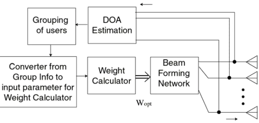
In the proposed algorithm, firstly, BS determines the MSs’ position, and categorizes the MSs into several groups in accordance with the distribution of MSs. Then, from several information contained in each group such as width and direction of each group and so on, the author determines the simple input parameters for the calculation method of the optimum weight vector for each array antenna by the proposed parameter setting method. After then, BS configures the required zone using the optimum weight vector. Figure 3.3 and 3.4
illustrates the image of the cellular radio system using proposed DZC technique, and an example of configuration of BS, respectively.
The main advantage to use the grouping technique is that making possible to suppress the maximum number of antenna beams to cover all MSs in a cell within the ability of array antenna at BS. In addition to this advantage, the tracking speed can be stabilized within a constant time by using a proposed parameter setting method from several information in each group into the input parameters for the calculation method of the optimum weight vector.
These advantages can be achieved only by making group for all MSs, determining input parameters for the calculation of weight vector by a fixed conversion map and calculating optimum weight vector regardless the number of MSs.
(a) Omni zone (b) Dynamic zone
Fig. 3.3 Omni vs. dynamic zone configuration.
Fig. 3.4 A example of configuration of BS.
In order to realize the grouping based DZC technique, following three algorithms must be clarified,
i) Determination algorithm of MSs’ position, ii) Grouping algorithm for MSs’ distribution,
iii) Parameter setting method to convert the several parameters related to the shape of each group into the input parameter to calculate the optimum weight vector.
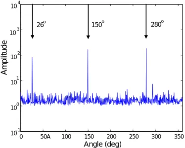
As for i), in this chapter, the author does not define the method, because a lot of methods to estimate direction of arrival (DOA) estimation have been studied [13]. Thus, the author only shows an example result using a multiple signal classification (MUSIC) method [14-16]
in Fig. 5. In this example, it is assumed that the developed 8-element circular array antenna receives 3 binary phase shift keying (BPSK) signals arrived from 26o, 150o and 280o simultaneously under no multipath environment. The center frequency is settled at 2.335 GHz, and the signal-to-noise ratio (SNR) of all signals equal to 5dB. With MUSIC method, the MS directions are correctly identified. Using the DOA estimation results, BS searches the MS’s position who is requesting a new call, requesting a handover, or terminating a call.
As for ii) and iii), in processing order at BS, firstly ii) and then iii) are explained. However,
in the first place, the author must define the method for calculation of optimum weight vector.
Therefore, first, the optimum weight vectors at each parameter were calculated in order to establish the invariable parameter setting method for the required number and direction of beams, by using eq. (3.4) and s(φ), and changing all the parameters such as Nd, Nu, θ, g, ψ, α and β. Second, the relationship between the setting parameters and the configured zone shape was investigated from the viewpoint of the directions, width, and number of antenna beam patterns [11]. Third, the author searched the setting parameters which can minimize the difference between the desired zone shape and the configured zone shape. Fourth, the method for parameter setting is fixed. It only requires the number of the required beams and a few information. Finally, using this fixed parameter setting method, the grouping algorithm was investigated. Therefore firstly iii) and then ii) are explained.
0 50A 100 150 200 250 300 350
10 -1 10 0 10 1 10 2 10 4
Angle (deg)
Amplitude
10 3
26 o 150o 280o
Fig. 3.5 The DOA estimation using the array antenna and MUSIC method for MS directions of 26 o, 150o, and 280 o. (The length of sample = 1000, SNR = 5 for all signals.)
3.3.3. A Method for Parameter Setting
In this section, the author defines the method for parameter setting, which converts the grouping information performed by the grouping algorithm for MSs’ distribution into the input parameters for eq. (3.4). To make the input parameters for eq. (3.4) as soon as possible, the simple and unique parameter setting method must be determined for the number and directions of the required antenna beams.
Nevertheless, it is difficult to obtain such a good setting method, because the number of the set of input parameters for eq. (3.4) to make the required zone shape is infinite. Therefore, first, several kinds of optimum weight vectors are calculated by using eq. (3.4) and s(φ) and changing all the parameters such as Nd, Nu, θ, g, ψ, α and β. Then, the accuracy of the configured beam shape was evaluated by comparing the number and direction of setting antenna beam pattern for more than 100 samples[11]. As a result, a conversion map to make n beams was found. It is unique for the number of the required beams. In the proposed parameter setting, the maximum number of groups is 4 in order to reduce the complexity. The parameter setting method is given as follows:
[For one group configuration] BS sets the parameters as listed in Table 3.2.
[For two groups configuration] BS sets the parameters as listed in Table 3.3.
[For three groups configuration] BS sets the parameters as listed in Table 3.4.
[For four groups configuration] BS sets the parameters as listed in Table 3.5.
Table 3.2. Parameters for one group.
Nd θ Gain Nu ψ α β
5 ϕ 1 - x1 /2 ϕ 1 – x1 /4
ϕ 1
ϕ 1 + x1 /4 ϕ 1 + x1 /2
ε × ξ 1
ξ 1
ξ 1
ξ 1
ε × ξ 1
2 ϕ 1 –10- x1 /2 ϕ 1+10+ x1 /2
0.1 0.1
Table 3.3. Parameters for two groups.
Group Nd θ gain Nu ψ α β
1 10 ϕ 1 – x1 /2 ϕ 1 – x1 /4
ϕ 1
ϕ 1 + x1 /4 ϕ 1 + x1 /2
ε × ξ 1
ξ 1
ξ 1
ξ 1
ε × ξ 1
4 ϕ 1 –10- x1 /2 ϕ 1+10+ x1 /2
0.1 0.1
2 ϕ 2 - x2 /2 ϕ 2 - x2 /4
ϕ 2
ϕ 2 + x2 /4 ϕ 2 + x2 /2
ε × ξ 2
ξ 2
ξ 2
ξ 2
ε × ξ 2
ϕ 2 –10- x2 /2 ϕ 2+10+ x2 /2
Table 3.4. Parameters for four groups.
Group Nd θ gain Nu ψ α β
1 3 ϕ 1 ξ 1 3 ( ϕ 1 + ϕ 2 )/2 0.1 0.1 2 ϕ 2 ξ 2 ( ϕ 2 + ϕ 3 )/2
3 ϕ 3 ξ3 ( ϕ 3 + ϕ 1 )/2
Table 3.5. Parameters for four groups.
Group Nd θ gain Nu ψ α β
1 4 ϕ 1 ξ 1 4 ( ϕ 1 + ϕ 2 )/2 0.1 0.1 2 ϕ 2 ξ 2 ( ϕ 2 + ϕ 3 )/2
3 ϕ 3 ξ3 ( ϕ 3 + ϕ 4 )/2 4 ϕ 4 ξ4 ( ϕ 4 + ϕ 1 )/2
Here, the parameters ϕ i , ρ i , and R i indicate the information of the shape of MSs group as follows:
ϕ i : The center direction of the ith group [degree], ρ i : The width of the ith group [degree],
R i : The distance between BS and the farthest MS from BS of the ith group.
Further, to convert the information of the shape of MSs group to the input parameters for eq. (3.4), x i , ξ i , and ε are defined as follows:
x i : The parameter, that relates to ρ i , to control the width of the beam for the ith group [degree],
ξ i : The parameter, that relates to R i , to control the size of the beam for the ith group, ε : The attenuation factor.
Figure 3.6 shows an example of the relationship between the center direction and the width of a group in the case of n =1. In this figure, BS categorizes the MSs into one group, in which the width and the center direction is ρ1 and ϕ1 degrees, respectively. The distance of the farthest MS from BS is R1. In this case, the parameters are set as Nd =5, θ = [ϕ1-x1/2, ϕ1-x1/4, ϕ1+x1/4, ϕ1+x1/2], g = [ε×ξ1, ξ1, ξ 1, ξ 1, ε ×ξ1], Nu =2, ψ = [ϕ1-10-x1/2, ϕ1+10+x1/2], α =0.1, and β =0.1 to eq. (3.4) (See Table 3.2.). Then the optimum weight vector wopt is
obtained and finally a beam pattern which can cover all MSs in one group is configured. In this parameter setting, how to decide the parameters x i, ξ i, and ε is quite important. Therefore they are explained in detail at the following subsections.
Fig. 3.6. Relationship between center direction and width of a group.
3.3.3.1 The relationship between the setting beam width and the configured beam width As shown in Table 3.2 or 3.3, in the case of configuring one group and two groups, BS forms the zone shape by accounting the group width. And the value of θ and ψ utilize x i, which is a setting parameter related to the width of the group as shown in Table 3.2 and Table 3.3. Here, the beam width is defined as under 3 dB from the peak. In the calculation of the optimum weight vector, from the previous research [11], the relationship between x i and the beam width ρ i is given as follows:
ρ i = A x i2 + B x i + C. (3.7)
In the case of configuring one group, A ≈ -0.0018, B ≈ 1.3300, and C ≈ -10.726 obtains optimum beam width.
eq. (3.4), x1 and x2 are assumed as the same value. In this case, the value of A, B, and, C depends on the difference of directions between two beams |ϕ1 - ϕ2|. Table 3.6 lists a result of the relationship between the values of |ϕ1 - ϕ2|, A, B and C in eq. (3.4). If |ϕ1 - ϕ2| is different from the value listed in Table 3.6, A, B, and C are selected from the listed value closest to given |ϕ1 - ϕ2|.
In the case of three groups and four groups, θ and ψ are not related to the value of the group width to reduce the complexity. Needless to say, the ability of the configurable zone shapes is limited.
Table 3.6. Coefficients for two groups.
| ϕ1 -ϕ 2 | A B C
90 -0.0156 3.0332 -48.117 100 -0.0104 2.8295 -44.620 110 -0.0249 4.2439 -78.415 120 -0.0224 4.0766 -86.142 130 -0.0267 5.0327 -138.15 140 -0.0172 3.6275 -87.647 150 -0.0108 2.5892 -45.668
160 -0.0002 1.1385 0.0392
170 0.0004 0.9496 7.7582
180 -0.0003 1.0017 6.6391
3.3.3.2 The gain parameter
Parameter ξi described in Table 3.2, Table 3.3, Table 3.4, and Table 3.5 are settled to determine the size of the beam for each group. At group i, ξ i is given by
(
/ max)
, 1 ,i R Ri i n
ξ = = … (3.8)
where Rmax is the largest value among Ri values (i = 1 .. n ). In the case of configuring one group, ξ1 = 1.
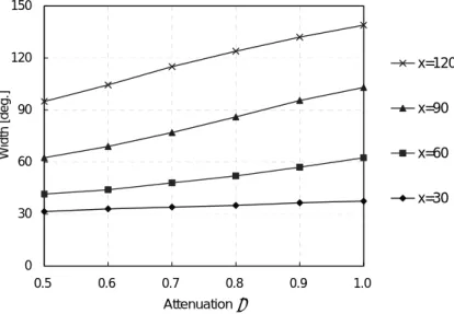
Parameter ε described in Table 3.2 and Table 3.3 is the attenuation factor to forming an antenna beam with required width (0<ε≤1). Figure 3.7 shows the relationship of ε and the configured beam width ρ1 when n = 1. The width of beam changes by changing ε, regardless of the value of x. To reduce the complexity of calculation, in this study, the author set ε = 0.8.
0 30 60 90 120 150
0.5 0.6 0.7 0.8 0.9 1.0
Attenuation ε
Width [deg.]
x=120
x=90
x=60
x=30
Fig. 3.7 Relationship between the attenuation parameter ε and beam width for desired direction when n = 1.
3.3.4 A Grouping Algorithm
By using the parameter setting algorithms described in Sec. 3.3.3 and eq. (3.4) with s(φ) shown in Table 3.1, the relationship between the setting parameters and configured zone shapes were examined. From the results, the author establishes the conditions to categorize one group, two groups, three groups, four groups or omni zone by the information of MSs’
distribution. Figure 3.8 shows a flowchart to determine the number of groups. In this
[One group] If BS can categorize the MSs into one group, and the width of the group is smaller than 137.5o, BS can configure a beam to cover the MSs.
[Ground] By substituting the parameters for the configuration of one beam in Table 3.2 and s(φ) for eq. (3.4), several weight vectors are calculated as a function of ϕ1and x to configure several beam patterns. In this case, by changing x, the maximum configurable beam width of ρ1 are derived [11]. As a result, the maximum beam width was determined to be 137.5o. In other words, with proposed parameter setting, a beam with the beam width of less than 137.5o is configured. Consequently, 137.5o is defined as the threshold value for the configuration of one group.
[Two groups] If BS can categorize the MSs into two groups with the direction of ϕ1,ϕ2, and the maximum beam width of the both groups is smaller than the threshold value, which depends on |ϕ1 - ϕ2| listed in Table 3.7, BS can configure two beams to cover the MSs.
[Ground] By substituting the parameters for the configuration of two beams in Table 3.3 and s(φ) for eq. (3.4), several weight vectors are calculated as a function of ϕ1, ϕ2, and x1 (=x2) to configure several kinds of beam patterns In this case, the width of each configured beam must be smaller than |ϕ1 - ϕ2|. Otherwise, one beam overlaps with other beam. Under this condition, the maximum configurable beam width of ρ1 and ρ2 are derived by changing several parameter such as x1 , x2, ϕ1, and ϕ2 [11]. In this calculation, x1 = x2 is assumed as shown in sec. 3.3.3. As a result, the relationship between |ϕ1 - ϕ2| and the configurable maximum beam width of ρ1 and ρ2 are determined as shown in Table 3.7. This relationship states that, proposed parameter setting invariably configures two beams with the beam width less than the listed minimum value between ρ1max and ρ2max in Table 3.7. |ϕ1 - ϕ2| is the condition to configure two groups. For example, in the case of |ϕ1 - ϕ2| = 90o, the parameter setting method can configure the 2 beams less than 73.0o. In other words, if the MSs is categorized
into two groups, and |ϕ1 - ϕ2| = 90o, and ρ1, ρ2 < 73o, the parameter setting method can make 2 beams.
[Three groups] If BS can categorize the MSs into three groups with the directions of ϕ1,ϕ2
and ϕ3 , and the maximum beam width of each group is smaller than 31o, and the conditions of 100 o ≤ |ϕ1 - ϕ2| and |ϕ2 - ϕ3| ≤ 160 o are met, then BS can configure three beams to cover the MSs.
[Ground] The same procedure was performed as in the case of two groups. First of all, the relationship between |ϕ1 - ϕ2|, |ϕ2 - ϕ3|, and the configurable maximum beam width of ρ1, ρ2, and ρ3 were obtained by using Table 3.4, s(φ), and eq. (3.4), by changing the value of ϕ1, ϕ2, and ϕ3 . Then, the maximum configured beam width ρ1, ρ2, and ρ3 without overlap were derived [11]. The results are shown in Table 3.8. As shown in Table 3.8, the proposed parameter setting invariably configures 3 beams with the beam width 31o, under the condition of 100 o ≤ |ϕ1 - ϕ2| , |ϕ2 - ϕ3| ≤ 160 o. Consequently, these results are defined as conditions to configure three groups.
[Four groups] If BS can categorize the MSs into four groups with the directions of ϕ1, ϕ2, ϕ3, and ϕ4 , and the maximum beam width of each group is smaller than 33o, and the confitions of 80o ≤ |ϕ1 - ϕ2| , |ϕ2 - ϕ3| , |ϕ3 - ϕ4| ≤ 100 o are met, then BS can configure four beams to cover the MSs.
[Ground] The same procedure was performed as in the case of two and three groups. First of all, the relationship between |ϕ1 - ϕ2|, |ϕ2 - ϕ3|, |ϕ3 - ϕ4|, and the configurable maximum beam width of ρ1, ρ2, ρ3, and ρ4 were obtained by using Table 3.5, s(φ), and eq. (3.4), and by
ϕ ϕ ϕ ϕ ρ ρ
proposed parameter setting invariably configures 4 beams with the beam width less than 33o, under the condition of 80o ≤ |ϕ1 - ϕ2| , |ϕ2 - ϕ3| , |ϕ3 - ϕ4| ≤ 100 o. Consequently, the these results are defined to configure four groups.
[Omni ] Otherwise.
Fig. 3.8 Algorithm for determining the number of groups.
Table 3.7. Relationship between |ϕ1 - ϕ2|, ρ1max,ρ2max, and minimum width between ρ1max, and ρ2max, in the configuration of two groups.
| ϕ 1 -ϕ 2 | [degree] ρ1max [degree] ρ2max [degree] Minimum width [degree]
90.0 85.5 73.0 73.0
100.0 96.5 68.0 68.0
110.0 99.5 74.5 74.5
120.0 103.0 82.5 82.5
130.0 93.5 89.0 89.0
140.0 88.0 100.5 88.0
150.0 87.0 143.0 87.0
160.0 147.5 140.5 140.5
170.0 162.0 151.0 151.0
180.0 159.0 157.0 157.0
Table 3.8. Relationship between |ϕ1 - ϕ2|, |ϕ2 - ϕ3|, and minimum width in the configuration of three groups.
| ϕ 1 -ϕ 2 | [degree] | ϕ 2 -ϕ 3 | [degree] Minimum width [degree]
100 100 32.0
110 32.5 120 32.5 130 31.5 140 32.5 150 31.5 160 32.0
110 100 33.0
110 33.0 120 31.5 130 32.0 140 31.0 150 32.0
120 100 32.0
110 32.5 120 31.0 130 31.5 140 32.0
130 100 32.0
110 31.0 120 32.0 130 33.0
140 100 31.0
110 33.0 120 35.0
150 100 33.5
110 33.5
160 100 33.5
Table 3.9. Relationship between |ϕ1 - ϕ2|, |ϕ2 - ϕ3|, |ϕ3 - ϕ4|, and minimum width in the configuration of four groups.
| ϕ 1 -ϕ 2 | [degree]
| ϕ 2 -ϕ 3 | [degree]
| ϕ 3 -ϕ 4 | [degree]
Minimum width [degree]
80.0 80.0 80.0 38.5
90.0 34.5
100.0 34.0
90.0 80.0 35.5
90.0 34.0
100.0 34.0
100.0 80.0 35.0
90.0 34.5
100.0 36.0
90.0 80.0 80.0 35.0
90.0 34.0
100.0 34.5
90.0 80.0 34.5
90.0 34.0
100.0 35.5
100.0 80.0 34.5
90.0 34.5
100.0 80.0 80.0 35.0
90.0 33.0
100.0 35.0
90.0 80.0 34.5
90.0 34.5
100.0 80.0 35.0
3.3.5 Power Control
The method and the algorithm discussed above enable us to derive the suitable weight vector wopt in order to configure the beam toward to the MSs’ groups. Next, the transmission power must be defined to radiate from BS in order to transmit the required power to the MSs.
In order to communicate with all the MSs in a cell, BS needs to transmit signals with power adjust to the farthest MS in a cell. At the position of the farthest MS, the received power level Pr [dBm] from BS is given by
10 10
10log ( ) 10log ,
r p
P = T +d φ − χ−γ +σ (3.9)
where Tp [mW] is the injection power for array antenna, d(φ)[dB] is the antenna gain for the direction φ compared with the omni antenna, χ is the distance from BS to the farthest MS, γ is the propagation factor and σ is the standard deviation of the short term median value variation caused by fading. Here, zo and M [dBm] are defined as the radius of a cell and the required signal level at cell boundary, respectively. The total radiation power for the direction φ, which is multiplied Tp and antenna gain, can be written as follows:
10 10
10log p ( ) 10log o ,
M = T +d φ − z −γ +σ (3.10)
( ) 10 log10
10 10
10 10 .
d zo M
Tp
φ γ+ −σ
× = (3.11)
For omni antennas, d(φ) equals to zero [dB] regardless of the direction φ, therefore the transmission power PO [mW] at BS is as follows:
( )
1 10 1
10 ,
2 2
d
O p p
P T d T d
φ
φ φ
φ φ
π π
=
∫
× =∫
(3.12)On the other hand, for DZC, the antenna gain dD(φ)[dB] for the direction φ is written using
the weight vector wopt:
2
( ) 10log10 H ( ) .
D opt
d φ = w s φ (3.13)
By using DZC, it is assumed that a constant level from BS is transmitted to the farthest MS using DZC. Letting that the farthest MS is at the direction φ with distance of R0 from the BS and receiving a constant level of power M. The total radiation power for the direction φ, which is multiplied with the injection power Tp’ to configure DZC and antenna gain can be written as follows:
10 10
10log p' D( ) 10log o ,
M = T +d φ − R−γ +σ (3.14)
( ) 10 log10
10 10
' 10 10 .
D o
d R M
Tp
φ γ+ −σ
× = (3.15)
Therefore the transmission power PD [mW] at BS is as follows:
( )
1 10
' 10 .
2
dD
D P
P T d
φ φ
π φ
=
∫
× (3.16)The ratio of the transmission power PD for DZC to the transmission power PO is defined as the transmission power ratio.
3.3.6. Channel Assignment Strategy
In addition to the proposal of a new DZC technique, in order to increase the system performance, the effectiveness to combine DZC with dynamic channel assignment (DCA) strategy is investigated. In this subsection, the principle of DCA is explained briefly. DCA can be roughly classified as either conventional DCA (CDCA) or distributed DCA (DDCA).
down-link are satisfied [17]. Various strategies for designing DDCA have been proposed. In the simulation, autonomous reuse partitioning (ARP) is applied [18][19], a typical DDCA method that works as follows:
1) An identical sequence of channels is given to all BSs in advance.
2) When a call attempt arrives at a BS, the channels are checked in a predetermined order. The first idle channel that satisfies CIRcall for both links is allocated.
3) If no channel are available, the call is blocked.
3.4. Computer Simulation Results
In order to investigate the effectiveness of the proposed DZC technique and the combination of DZC and DCA, the computer simulation is performed.
3.4.1. System Model
In the computer simulation model, each BS uses two zones: one zone is for control channel used to grasp the positions of MSs, and the other zone is for communication channel used to communicate between BS and MSs. These zones are called the “control zone” and the
“communication zone”, respectively, and these are shown in Fig. 3.9. The control zone has an omni-directional shape and is equal to or larger than the size of each cellular zone. Its radius assumes z times larger than each cellular zone. Using the control channel, the BS searches for the active MSs requesting a new call, requesting handover from an adjacent zone, or terminating a call. Then, by using the information of MSs’ position and the proposed DZC technique, BS configures the required communication zone by an 8-element array antenna. In this computer simulation, a narrow-band FDMA-FDD mobile communication system is assumed and the system performance is evaluated. Here, although the method that provide the DOA estimation is not defined, by using a DOA estimation method as mentioned in
subsec. 3.3.2, it is assumed that BS has already known the MSs’ position in advance, in the simulation.
Control zone Communication
zone
(a) z=1 (b) z=2
Fig. 3.9 Communication zone configuration when (a) z=1 and (b) z=2.
3.4.2. Simulation Model
(a) The simulated service area was two-dimensional, there were 196 (14×14) cells, and system performance were investigated in the 64 (8×8) cells around the center of the service area (See Fig. 3.10(a)).
(b) In order to simulate the proposed system in not only uniformly distributed traffic environment but also non-uniformly distributed traffic environment, some cellulars is assumed as non-uniformly distributed traffic cells. In this simulation, the non-uniformly distributed traffic cells is arranged as shown in Fig. 3.10(a). As a result, in the simulated service area, there were 147 uniformly distributed traffic cells and 49 non-uniformly distributed traffic cells.
(c) The traffic in the uniformly distributed cells was assumed as six erl/cell. In the non-uniformly distributed traffic cells, the traffic in one-sixth area of each cell was u
total traffic of non-uniformly distributed traffic cell is (u +5) erl/cell, and the high-traffic area with u erl/cell was randomly located in each cell as shown in Fig.
3.10(b).
(d) Call attempts from MSs were generated as a Poisson process in time. Call duration was assumed to have an exponential distribution with a mean of 120 seconds.
(e) The total number of FDMA channels is 70 for the up-link and for the down-link, respectively, and in the case of FCA, these frequency channels are reused every 7 cells.
(f) Propagation factor γ was 3.4, the standard deviation of the short term median value variation caused by fading σ was a 6.5 [dB], and the required power M [dBm] at the farthest MS from BS was 0.
(g) MSs were at a standstill (i.e., speed = 0 km/h).
(h) CIRcall =15 dB and a CIRover = 10 dB. The CIRover is the threshold CIR value for the changing of channel. If CIR of up-link or down-link is less than CIRover, MSs must try to get new channels.
(i) The radius of the omni cell z0 was 1 km.
(j) z was 1 or 2 (see Fig. 3.10).
(k) The BS changed the zone shape when a MS attempted a new call, terminated a call, or requested a handover.
Uniform distributed traffic area Non-uniform distributed traffic area
(a) The arrangement of the non-uniform distributed traffic cell and the uniform distributed traffic cell
5 erl
u erl High Traffic
Area
(b) The traffic distribution in the non-uniform distributed traffic cell Fig. 3.10 Service area model.
The simulation was carried out as follows (See Fig. 3.11): when a MS generates a call attempt or a handover request, the MS contact to the nearest BS. The BS looked for an available channel. If a channel was available, the BS checked the position of all MS communicating with the BS, Then BS created a communication zone by using the proposed method and algorithm. If no channel were available and the MS was in a control zone covered by one or more neighbor BSs, the BS told the MS to contact the neighbor BSs in
Fig. 3.11 Flowchart for channel allocation using the method.
3.4.3. Numerical Results
An example of communication zone configuration generated in the simulation is shown in Fig. 3.12. The relationship between the offered load over the high-traffic area and the blocking rate (BR) is shown in Fig. 3.13. The DZC technique had the lowest BR regardless of the channel allocation algorithm. Especially, with ARP, the BR was remarkably lower than with the omni-zone technique for z = 2. The forced call termination rate (FCTR) under the same condition is shown in Fig. 3.14. With FCA, the DZC technique had a higher FCTR than with the omni-zone technique. On the other hand, with ARP, the DZC technique had a lower
FCTR than with the omni-zone technique, in particular for z = 2. Figure 3.15 shows the transmission power ratio needed to configure the communication zone. When z = 1, the required transmission power less than one-half of the one needed for the omni-zone system.
When z = 2, the transmission power is larger than z = 1, because the BS also covers MSs who have crossed the present cell boundary. However, by using ARP the transmission power can be kept at a low level because the BS can assign channels dynamically over cells according to the channel demands without changing the zone shape.
Fig. 3.12 Example of communication zone configuration.
1.E-04 1.E-03 1.E-02 1.E-01 1.E+00
1 5 9 13 17 21
Offered load over high traffic area u
Blocking Rate
Omni (FCA) DZC (z=1) (FCA) DZC (z=2) (FCA) Omni (ARP) DZC (z=1) (ARP) DZC (z=2) (ARP)
1.E-06 1.E-05 1.E-04 1.E-03 1.E-02 1.E-01 1.E+00
1 5 9 13 17 21
Offered load over high traffic area u
Forced Call Termination Rate
Omni (FCA) DZC (z=1) (FCA) DZC (z=2) (FCA) Omni (ARP) DZC (z=1) (ARP) DZC (z=2) (ARP)
0 0.5 1 1.5 2 2.5 3
1 5 9 13 17 21
Offered load over high traffic area u
Transmission Power Ratio
DZC (z=1) (FCA) DZC (z=2) (FCA) DZC (z=1) (ARP) DZC (z=2) (ARP)
Fig. 3.14 Forced call termination rate.
Fig. 3.13 Blocking rate.
Fig. 3.15 Transmission power ratio.
3.4.4. Discussion
In this subsection, the results obtained from Figs. 3.13, 3.14 and 3.15 are discussed more deeply. From Figs. 3.13 and 3.14, the both of BR and FCTR are improved by combining DZC technique and DCA strategy. This is equivalent to the achievement of the effectively utilization of the radio spectrum. In order to investigate the frequency utilization efficiency, firstly the performance of BR was calculated in omni zone system with the total FDMA channel of 70 as shown in Fig. 3.13. Then, BR of DZC technique (z=2) was calculated by changing the number of total FDMA channel, and searched the number of channels to obtain the same BR of omni zone environment with 70 channels under the same traffic (u =1). As a result, by using 49 FDMA channels, the same BR performance of omni zone system is obtained. In the case of the combination between the DZC and ARP (u =1), the number of FDMA channels is reduced to 29. Of course, the efficiency also depends on the algorithm of DCA. For example, when the First Available (FA) [17][18] is applied, the same BR performance is achieved with the total FDMA channels of 33.
Next, the author discusses the reason that the efficiency of DZC is smaller than DCA as mention in above subsection. As a reason, it is thought that the simulation uses FDMA-FDD and MSs utilize omni directional antenna. By using DZC technique, in the down-link from BS to MSs, the MSs can suppress to receive the undesired wave and improve CIR. However, for the up-link, MSs assume to use omni directional antenna and can’t improve CIR in comparison with down link. BR and FCTR are dependent on the CIR of up-link. Therefore large improvement of BR and FCTR can not be obtained.
Further, the author discusses the influence of the number of FDMA channels. If the number of FDMA channels is increased, under the fixed traffic, BS can use large number of
offered load is increased under the fixed number of FDMA channels, in each cell, the distribution of MSs becomes to uniformly distributed and BS tends to select omni zone by DZC. Therefore the difference of BR and FCTR between DZC and Omni is almost same.
In this chapter, the efficiency is investigated when z = 1 and z = 2 shown in Fig 3.9. When z=2, the system performs better than those of when z=1. This is because the BS is able to
cover the MSs in neighbor cells and smooth out the spatial traffic unbalance when z = 2.
However in the case that the traffic is large, BS tends to make large zone when z = 2.
Consequently, BS needs the large transmission power, and increases FCTR because of the increase of co-channel interference. In the near future the investigation of optimum z is required.
3.5. Conclusion
In this chapter, in order to implement a dynamic zone configuration technique into cellular mobile communication systems, the author proposed a simplified method and algorithm for determining the suitable weight vector based on the LS method. In the all calculations, the system model with developed prototype antenna was assumed. Then system performance such as BR and FCTR was evaluated by introducing the proposed dynamic zone configuration technique to FDMA-FDD system. Moreover, the effectiveness combining the dynamic zone configuration technique with the dynamic channel assignment strategy was investigated. From the simulation results, it was found that the dynamic zone configuration technique with dynamic channel assignment strategy was more effective in controlling blocking rate (BR), forced call termination ratio (FCTR), and transmission power ratio in compared with that of omni zone. Further work will include investigation under the situation that MSs move.