Bipartite Graphs in 3D
Takao Ito, Kazuo Misue and Jiro Tanaka Department of Computer Science, University of Tsukuba,
Tennodai, Tsukuba, 305-8577 Ibaraki, Japan [email protected] {misue,jiro}@cs.tsukuba.ac.jp
Abstract. Circular anchored maps have been proposed as a drawing technique to acquire knowledge from bipartite graphs, where nodes in one set are arranged on a circumference. However, the readability decreases when large- scale graphs are drawn. To maintain the readability in drawing large-scale graphs, we developed “sphere anchored maps,” in which nodes in one set are arranged on a sphere. We describe the layout method for sphere anchored maps and the results of our user study. The results of our study revealed that more clusters of free nodes can be found using sphere anchored maps than using circular anchored maps. Thus, our maps have high readability, particularly around anchors.
1 Introduction
Information with bipartite graph structures can be seen in various real-world areas, for example, customers and products, web pages and visitors, or papers and authors.
This information often has a large-scale graph structure. Visualizing this information is an efficient method of analysis. However, conventional visualization techniques for bipartite graphs [1-5] do not provide enough readability for drawing large-scale graphs.
“Anchored maps [1,2]” have been proposed as an effective drawing technique to acquire the knowledge from bipartite graphs. Nodes in one set are called “anchors,”
and nodes in another set are called “free nodes” (They can be exchanged).Anchors are arranged on a circumference, and free nodes are arranged at suitable positions in relation to adjacent anchors. For convenience, we call this visualization technique
“circular anchored maps (CAMs)” in this paper.
When large-scale graphs are drawn, the readability particularly around the anchors is low on the CAMs (Fig. 1). We think that arranging anchors on the circumference causes low readability in the CAMs. Thus, to increase the readability, we extend them by arranging anchors on a sphere that has 2D layout space while keeping their features. We call this visualization technique “sphere anchored maps (SAMs).”
In this paper, we describe the features of SAMs and a layout method developed to
satisfy their aesthetic criteria. Additionally, we show the results of a user study to
evaluate the readability around anchors.
2 Related Work
Zheng et al. [3] proposed two layout models for bipartite graphs and proved theorems of edge crossing for these models. Giacomo et al. [4] proposed drawing bipartite graphs on two curves so that the edges do not cross. Newton et al. [5] proposed new heuristics for two-sided bipartite graph drawing. We describe a new visualization technique for large-scale bipartite graphs to maintain high readability.
Related work on 3D visualization includes a study in which Munzner et al. [6]
developed H3, which lays out trees on 3D hyperbolic space with high readability. Ho et al. [7] developed drawing techniques that lay out clustered graphs in which each cluster is arranged on a 2D plane and in which a parent graph of clusters is laid out in 3D. We developed a drawing technique for bipartite graphs in 3D.
3 Circular Anchored Maps and Existing Problems
CAMs have been proposed as a drawing technique of anchored maps for bipartite graphs [1]. CAMs arrange anchors on the circumference at equal intervals and free nodes by spring embedding [8]. CAMs have the following features:
• The positions of free nodes are understandable in relation to the anchors. The anchors are fixed on the circumference at equal intervals, which produces an effect like the coordinate system.
• Clusters of free nodes can be discerned based on their relation to the anchors.
The free nodes are divided into clusters by the connective relationships with adjacent anchors. This illustrates what kinds of clusters exist and which anchor subset is responsible for constructing each cluster.
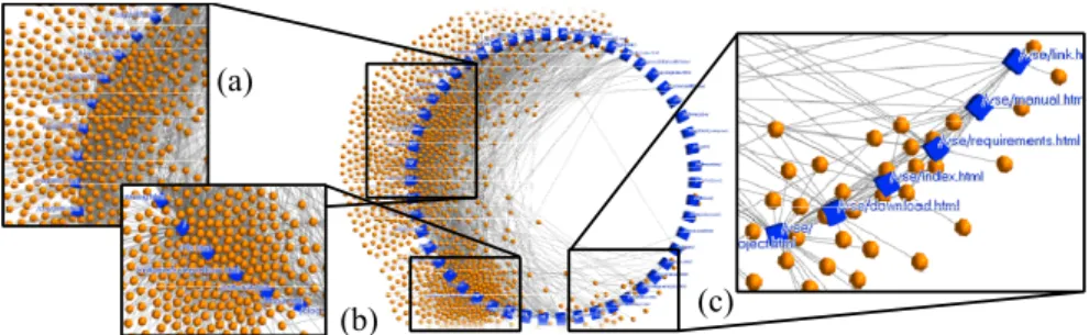
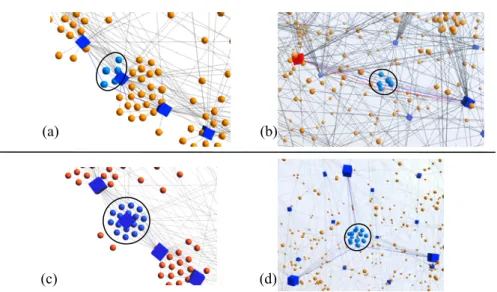
The readability of CAMs is low when large-scale graphs are drawn. Fig. 1 shows an example where a graph that has 52 anchors and 1137 free nodes was drawn as a CAM.
We focus particularly on problems where the readability around anchors is low.
Anchors are arranged in CAMs on the circumference that has only 1D layout space.
Thus, only two anchors can be adjacent to a certain anchor spatially, and the anchors' arrangement tends to become a straight line as the number of anchors increases.
Therefore, free nodes adjacent to anchors arranged closely are arranged on the circumference, and edges connected to these nodes become difficult to read (Fig.
1(c)). Additionally, clusters of free nodes around anchors are often mixed with other
clusters (Fig. 1 (a) and (b)).
Fig. 1. Drawn example of circular anchored map (CAM). Anchors are represented by rectangles (cubes). Free nodes are represented by circles (spheres).
4 Sphere Anchored Maps
We think that arranging anchors on a circumference that has a 1D layout space causes these problems. Thus, we arrange anchors on a sphere that has 2D layout space and free nodes in 3D space. In SAMs, anchors are arranged on the sphere, free nodes do not receive the restriction of the position, and edges are drawn using straight lines.
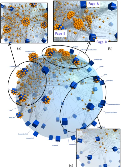
An example of a SAM is shown in Fig. 2. The same graph that is in Fig. 1 is drawn. This graph represents the relationships between a web page and visitors.
Anchors drawn by cubes mean web pages, and free nodes drawn by spheres mean visitors. The readability around anchors increases by extending anchors' layout space to 2D. Mixtures among clusters of free nodes are not caused because the layout space broadens. For example, Fig. 2 (b) has three large clusters of free nodes that are mixed in Fig. 1. It indicates that many visitors accessed pages A, B, and C, pages A and B, and pages A and C, but few visitors accessed pages B and C. Additionally, we can see that a cluster of free nodes in the center of Fig. 2 (c) connects to six anchors. We know that visitors that accessed one of the pages represented by these anchors tend to access others.
The occlusion of nodes in 3D visualization is a problem. We address this problem by rotating the drawn graph [9] based on the research by Ware et al. [10]. Sample videos are available from the first author's web site
1.
We use the following aesthetic criteria to develop layout methods for SAMs. These aesthetic criteria are extensions of aesthetic criteria of CAMs [1] and are important to keep their features.
• (R1) Nodes adjacent to each other are laid out as closely as possible.
• (R2) Anchors adjacent to common free nodes are laid out as closely as possible.
• (R3) Anchors are distributed on the sphere as evenly as possible.
We describe formal expressions for R1 and R2 because these are used later in this paper. Suppose that A is the set of anchors, F is the set of free nodes, P(n) is a 3D vector expressing a position of node n, and A(f) is the set of anchors adjacent to free
1
http://www.iplab.cs.tsukuba.ac.jp/~ito/
(a)
(b) (c)
( )
{ ∈ ∈ } { a
1, a
2, a
3,..., a
m}
Moreover, suppose that r is the radius of the sphere, and d ( n
1,n
2) is a Euclid distance between node n
1and node n
2.
Fig. 2. Drawn example of sphere anchored map (SAM). In this figure, (a), (b), and (c) correspond with (a), (b), and (c) in Fig. 1.
(a) (b)
(c)
R1 is to minimize l(E) expressed by:
∑
∈=
E f a
f a d E
l
) , (
) , ( )
( (1)
R2 is to minimize g(F) expressed by:
( ) ( )
∑ ∑
∈ ∈ <
−
⎟⎟
⎟
⎠
⎞
⎜⎜
⎜
⎝
⎛
⎟⎟ ⎠
⎜⎜ ⎞
⎝
⎛ •
=
F
f a a A f i j
j i
j
i
r
a F a
g
), (
, 2
1
P P
cos )
( (2)
In exp(1), l(E) indicates the total length of the edges. In exp(2), g(F) indicates the total length of the arc between anchors adjacent to the common free node. If the value of g(F) is small, the anchors adjacent to the common free node are laid out closely.
5 Layout Method
The layout method of anchors is important because the layout of anchors influences the readability of SAMs. In CAMs or two-sided graphs [5], we only consider the order of nodes. CAMs decide the order of anchors on the circumference (in other words, on the vertices of a regular polygon) by running an algorithm. However, the layout space of anchors in SAM is 2D. Therefore, deciding the position of the anchors is difficult.
We extended the layout-explore algorithm used in CAMs, in which the map is laid out according to the following three steps.
1. Candidate positions for anchors to satisfy aesthetic criterion R3 are obtained by considering anchors to be electrons and by simulating their behavior on the sphere.
2. The layout of anchors to satisfy aesthetic criteria R1 and R2 are explored using the layout-explore algorithm.
3. Free nodes are arranged using force-directed placement.
5.1 Candidate positions for anchors
In the first step, candidate positions for anchors to satisfy aesthetic criterion R3 are obtained. It is a hard problem called the “sphere packing problem [11,12].” However, our purpose was not to resolve this problem but to acquire a high-readability layout.
Thus, we obtained candidate positions for anchors by simulating “the behavior of electrons on the sphere.”
5.2 Layout-explore algorithm
In the second step, the layout-explore algorithm used in the CAMs computes a quasi-
optimal order of anchors for the penalty [1]. This algorithm repeatedly chooses two
comparison by choosing anchors far from each other, then shortens the distance between compared anchors, and finally compares adjoined anchors at the end. If the penalty does not decrease at a certain distance, the distance is cut in half. The algorithm continues until the distance becomes zero.
In the layout-explore algorithm used in the SAMs, the order near to a certain anchor is used as the distance.
We use l(E) or g(F) as the penalty. However, l(E) can be evaluated only after the position of free nodes has been decided. Therefore, we approximate the position of free nodes using the barycenter of adjacent anchors.
The layout-explore algorithm used in the SAMs is shown in Algorithm 1. Here, A is a set of anchors, currentPenalty is the function that returns the value of the current penalty, and NearFromA(a,d) is the function that returns the nearest d-th anchor from anchor a.
Algorithm 1
Algorithm 1 will definitely stop at some point because the penalty cannot keep decreasing infinitely, that is, the patterns of the layout of the anchors are finite.
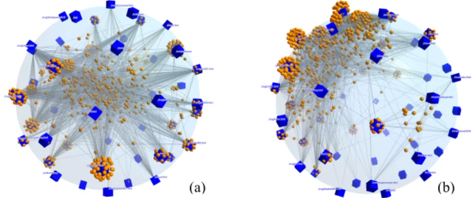
5.3 Efficacy of our layout method
The efficacy of our layout method is illustrated in Fig. 3. Fig. 3(a) shows a state where the anchor's arrangement candidate has been obtained (anchors are arranged at random). Fig. 3(b) shows the results of the layout-explore algorithm. In the random layout, most of the free nodes are arranged around the center of the sphere. As a result, free nodes that have no relationship with each other gather in the central part of
1 : double p0 = currentPenalty;
2 : int d = |A| - 1;
3 : while (d > 0) {
4 : boolean c = false;
5 : do {
6 : c = false;
7 : for (int i = 0; i < |A|; i++) { 8 : Swap A[i] for NearFromA(A[i],d);
9 : double p1 = currentPenalty;
10 : if (p1 < p0) {
11 : p0 = p1; c = true;
12 : } else {
13 : Swap A[i] for earFromA(A[i],d);
14 : } 15 : }
16 : } while (c);
17 : d = d / 2;
18 : }
the sphere. Fig. 3(b), wherein free nodes are arranged around the surface of the sphere, is an overview of the graph.
Fig. 3. (a) laid out at random. (b) laid out using the layout-explorer algorithm.
6 User Study
We implemented our technique in C#+Managed DirectX and performed a user study to evaluate the readability of the SAMs, particularly around anchors. The study included six participants.
We asked the participants to perform tasks using both a SAM and a CAM. A cluster of free nodes (F-cluster) is a set of free nodes that connect to the same anchors.
In this task, participants looked for all “target F-clusters,” which constituted five or more free nodes and were connected to two or more anchors, from a graph in a limited amount of time. When the participants found a F-cluster, they selected one of the free nodes in the F-cluster by right-clicking it, thereby highlighting the F-cluster.
Selected (highlighted) F-clusters could be unselected by right-clicking them again.
Participants translated anchored maps by middle-dragging, rotating them by right- dragging, zooming in/out using the mouse wheel, and controlling the edge opacity, size of anchors, and size of the free nodes using the left panel. The number of target F-clusters and selected F-clusters and the time remaining were shown at the upper left of the screen. When the number of target F-clusters equaled the number of selected F- clusters, a beep sounded. The time given was limited to 7 × the number of target F- clusters in seconds. After the participants found all the target F-clusters, they clicked a button, and the task was over. Fig. 4 shows screenshots of the test program.
Participants performed two tasks using the CAM and two tasks using the SAM as training. Then, they performed ten tasks each using the CAM and SAM. Three participants performed tasks using the previous CAM, and the others performed tasks using the previous SAM. The same graphs were used in both anchored maps.
Ten bipartite graphs used in the ten tasks were generated using the following procedure.
1. Generate 50 nodes laid out as anchors.
2. All anchors connect to 16 anchors through a node laid out as a free node. All anchors are 16 degrees, and all free nodes are 2 degrees.
3. Edges are replaced from 30 to 70 times at random.
(a) (b)
5. From 20 to 80 edges are added at random.
6. From 10 to 25 F-clusters are added at random. They have from 5 to 10 free nodes.
7. From 3 to 10 F-clusters are added at random. They have from 10 to 30 free nodes.
8. From 3 to 10 F-clusters are added at random. They have from 2 to 3 free nodes.
The generated graphs had 50 anchors, about 650 free nodes, about 1400 edges, and about 17 target F-clusters. F-clusters in these graphs tended to be arranged around anchors. The order of tasks was random.
6.1 Results
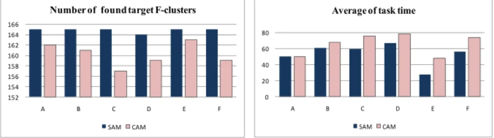
Fig. 5 shows the number of target F-clusters found in the time provided. The ten tasks had a total of 165 target F-clusters. While 160.8 target F-clusters were found using the CAM, 164.8 target F-clusters were found using the SAM. Five participants found all of the target F-clusters using the SAM. A paired t-test revealed a significant difference (p < 0.05, t=5.66).
Fig. 6 shows the task time. Five participants finished on time using the SAM, while all participants failed to finish on time using the CAM. We found a significant difference in a paired t-test (p < 0.05, t= -3.08).
Fig. 4. Screenshots of test program. The left image shows the test of the CAM, and the right image shows the test of the SAM. F-Clusters highlighted in green are F-clusters selected by the participants. The participants controlled the edge opacity, size of the
Fig. 5. Number of found target F-clusters.
The ordinate indicates the number of target F-clusters found by participants.
Fig. 6. Average task time (seconds). The ordinate indicates the average task time by participants.
0 20 40 60 80
A B C D E F
Average of task time
SAM CAM 152
154 156 158 160 162 164 166
A B C D E F
Number of found target F-clusters
SAM CAM