Hovering Control of Vectored Thrust Aerial Vehicles

Hovering Control of Vectored Thrust Aerial Vehicles

Makoto Kumon, Hugh Cover and Jayantha Katupitiya

Abstract— In this paper, a vectored thrust aerial vehi- cle(VTAV) that has three ducted fans is considered. Since ducted fans are powerful and effective in providing lift, they are suitable for thrusters of UAVs, but modeling their aerodynamic effects such as ram drag is very difficult. The VTAV has one ducted fan fixed to its body and two ducted fans that can be tilted in order to make rotational moments, which makes the system dynamics even more complicated. This paper focuses on giving a precise dynamical model that includes aerodynamic effects of ducted fans. Then it presents a hovering controller based on the dynamical model developed. Since the horizontal dynamics are under actuated, a switching control approach is introduced to realize a stabilizing controller. Numerical simulations prove the validity of the approach.

I. INTRODUCTION

This paper presents the mechanical design, dynamic mod- eling and the implementation of a hovering controller on a micro aerial vehicle powered by three ducted fans. Ducted fans are known to have high drag coefficients and the distribution of the required thrust into three smaller ducted fans partially help improve the drag coefficient. Due to the drag coefficients fast forward flight with small pitch angles is a challenge. The system presented in this paper overcomes these disadvantages through its design. The authors of this paper presents the detailed near hover modeling of the entire aircraft followed by the design of a controller for hovering.

On-Board Computer

Micro- Controller

PC (User)

AHRS Wi-Fi

RS-232

I2C Bus

Electronic Speed Controller PWM

(Speed)

DC motor controller Digital (Direction)

Ducted Fan DC Tilt Motor

DC motor controller

Tilt Gearbox

Main Battery (22.2v)

Secondary Battery (7.4v)

Gumstix Tilt System Power System

PWM Signal

(a) VTAV (b) Schematic of VTAV Fig. 1. VTAV

Ducted fan based systems have been attracting the at- tention of researchers in the recent past. The majority of the work has been directed to the modeling and control of single ducted fan which form some sort of an aircraft. An attempt to model and control a small ducted fan aircraft

J. Katupitiya is with School of Mechanical and Manufacturing Engi- neering, University of New South Wales, Sydney NSW 2052, Australia [email protected]

M. Kumon is with Department of Intelligent Mechanical Systems, Grad- uate School of Science and Technology, Kumamoto University, 2-39-1, Kurokami, Kumamoto, Japan [email protected]

through dynamic inversion is presented in [1], [2]. These two articles present the dynamics of a UAV with a single ducted fan. Control of a ducted fan against wind gusts in the presence of modeling uncertainties is presented in [3]

with a robust controller based on backstepping method. This ducted fan, however, has rotors rotating in opposite directions which allows the separation of yaw dynamics from the rest of the modeling. A multi-input, multi-output sliding mode based controller is presented in [4]. The work in [5] presents a dynamic model that controls the ducted fan vertically up for hovering and then transiting to a near horizontal travel to achieve fast forward flight assisted by control surfaces.

The work by [6] presents an alternative approach to achieve near hover through decoupling (the UAV has counter rotating fans) instead of using fully coupled high order dynamics.

Applications of ducted fan based systems are presented in [7], [8].

In contrast to the work mentioned above, this paper presents the modeling of an aircraft that has three ducted fans. Instead of using control surfaces, vectored thrusts are used to achieve flight and hovering. The paper is presented as follow: Section II presents the VTAV architecture. Section III presents the detailed dynamic modeling and Section IV presents the hovering controller. Section V shows the results of the numerical simulations and conclusions are made in Section VI.

II. S YSTEM D ESCRIPTION

As shown in Fig. 1(a), the aircraft configuration with three ducted fans were chosen to ensure directional properties that are useful in various applications of the aircraft. Clearly, the use of three ducted fans is not favourable when it comes to torque balance of the engines (ducted fans). The ducted fans used in this design are not counter rotating. However, unlike the rotors used in helicopters, due to the presence of a stator and a rotor in ducted fans, the engine torque that remains to be canceled is manageable. In the design presented, one engine is fixed to the frame and is located at the front end of the aircraft. The other two engines are located at the rear of the aircraft as shown in the Fig. 1(a).

The mounting locations of the three ducted fans form an

isosceles triangle. The orientations of the engines at the back

of the aircraft can be tilted about an axis that coincides with

the base of the isosceles triangle mentioned above, and hence

the thrusts generated by these engines are vectored and can

be controlled independently. Therefore, the aircraft is called

a Vectored Thrust Aerial Vehicle (VTAV). The VTAV has

five control inputs, namely; the speeds of the three engines,

the independent vectoring of the two rear engines. It has no

control surfaces.

This unique design has a number of advantages. First of all, the vectored thrusts are used to cancel the unbalanced engine torques. Next the VTAV has the ability to hoover stably. Then, the vectoring can be used to yaw the VTAV while maintaining its altitude and, zero roll and pitch with respect to a horizontal plane. This capability is especially useful in attack aircraft and the capability also can be used for evasion. Unlike helicopters, the VTAV can translate in a forward direction using vectored thrust without the need for non-zero pitch. Nevertheless, roll, pitch and yaw can be achieved during flight through engine thrust control. An Xsense

^r

Attitude and Heading Reference System (AHRS) provides sensing, including approximate GPS. Among the sensed quantities are all three gyro rates and the three accelerations. An onboard computer commands the speed controllers of the three engines and controls the tilt angles of the two rear engines. The same onboard computer acquires data from the Xsense system and transmits them to a base station for processing. A joystick controller that operates through the base station transmits control commands to the onboard computer. A schematic of the system architecture is shown in Fig. 1(b).

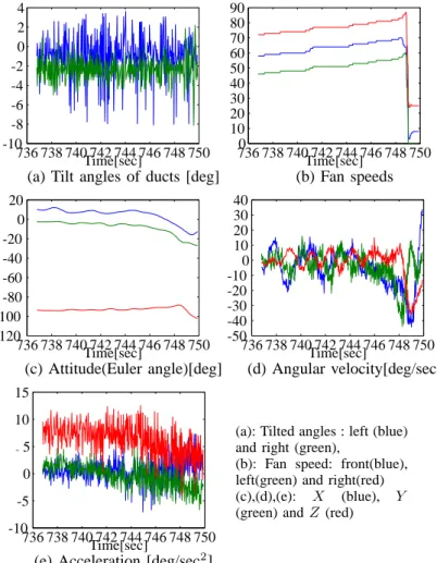
Actual manual flight data acquired are shown in Fig. 2. In this flight, VTAV was lightly tethered for safety reasons, and successfully flew in an indoor environment and showed that the configuration of the system was appropriately designed.

TABLE I S

PECIFICATION OF

VTAV

Mass: 3.5kg

Size(W×D×H): 420mm×355mm×95mm

Ducted-fan: MEGA, Moki EDF ACn 22/6s 94mm OD, 260g, 1.1kW

Servo motors: Maxon, RE10 1.5w 7.2v with Geerhead 1:16

AHRS: Xsens, MTi-G

Speed controller: Castle Creations, Phoenix-60 Onboard computer: Gumstix, Verdex Pro (PXA270)

with Robostix (ATMEGA128)

III. DYNAMICAL MODEL A. Rigid body model

The coordinate frames for a VTAV are defined as Σ I and Σ B which represent the inertial frame and the body frame respectively. Σ I is normally fixed on the terrain to show the location and the configuration of the VTAV, and Σ B is fixed to the body of the VTAV. The origin of Σ B corresponds to the centre of the mass and its X B axis is defined to align with the front direction. Z B axis is defined “downward” to the body and Y B axis is defined so as to make Σ B a right- hand system. Let symbols with subscripts I and B show quantities represented in Σ I and Σ B respectively. Denote the position and the configuration of VTAV by X I and Y I . Let a mapping of a vector in Σ I to that in Σ B as ^B T I . It is worth noting that it only depends on the configuration Y I . Denote translational velocity and angular velocity as V I and ω I respectively. Then the followings hold:

V B = ^B T I (Y I )V I (1) ω

B

= ^B T I (Y I )ω I (2)

Time[sec]

736 738 740 742 744 746 748 750 4

2 0 -4 -2 -6 -8 -10

Time[sec]

736 738 740 742 744 746 748 750 0 10

20 30 40 50 60 70 80 90

(a) Tilt angles of ducts [deg] (b) Fan speeds

Time[sec]

736 738 740 742 744 746 748 750 20

0 -20 -40 -60 -80 -100 -120

Time[sec]

736 738 740 742 744 746 748 750 0

-10 -20 -30 -40 -50 10 20 30 40

(c) Attitude(Euler angle)[deg] (d) Angular velocity[deg/sec]

2

Time[sec]

736 738 740 742 744 746 748 750 15

10 5 0 -5 -10

(a): Tilted angles : left (blue) and right (green),

(b): Fan speed: front(blue), left(green) and right(red) (c),(d),(e): X (blue), Y (green) and Z (red)

(e) Acceleration [deg/sec ² ]

Fig. 2. Flight Test Result

Control signals (tilt angles of ducts and fan speeds) are shown in the top two figures. Response of VTAV is shown in Fig.(c), (d) and (e) as its attitude, angular velocity and acceleration measured by on-board sensors.

Assuming that the VTAV can be modeled as a rigid body, denote the mass and the inertial tensor with respect to Σ B

as m and I B , where I B can be represented by a constant matrix. Motion equation can be expressed in the following form:

m d

dt V B + ω B × V B

= F B + m ^B T I (Y I )g _I (3) I B

d

dt ω B + ω B × I B ω B = N B , (4) where F B and N B show aerodynamic forces and moments described below, and g _I shows the gravitational acceleration with respect to Σ I . × shows vector product. X I and Y I

can be computed by (1) and (2), since velocities in them can be obtained by solving (3) and (4).

Denote the wind vector as W B and model it as

W B = ^B T I (W I − V I ) = ^B T I W I − V B . (5)

Let tilt angles of the two ducted-fans at the rear of VTAV be

θ 2 and θ 3 respectively, and those angles are measured from

Z B axis toward X B axis. The force generated by a ducted

fan is modeled based on models in references [9], [10] and

[11].

Duct 1 Duct 2

Duct 3 X B Y B

Z B

O B

W θ ₂

Inertial Frame Fig. 3. VTAV and coordinate frames

B. Ducted fan model

The fundamental model of a ducted fan is introduced first, then it is extended to the VTAV case.

1) Thrust: Thrust generated by a fan in a duct can be modeled by a discontinuous pressure drop at the fan which causes the flow through the duct(Fig. 4). Since the amount of the thrust is equal to the force to accelerate the air, thrust F T can be modeled as follows.

F T = π

4 A ² ρu(U + u

2 ), (6)

where U and u show the velocity of the air in the free- field and the induced velocity respectively. ρ and A show the density of the air and the diameter of the duct where the fan locates. The induced velocity u can be modeled to be proportional to the speed of the fan, which is denoted by ω.

Then, (6) can be rewritten as

F T = C ₁ U ω + C ₂ ω ² , (7) where C 1 and C 2 are constant coefficients. Note that the direction of F T is aligned with the flow, but opposite to it.

2) Ram drag: When there is a flow in the free-field not aligned with the duct as shown in Fig. 4(b), an additional aerodynamic force effects the duct, which is called ram drag.

This is counter force caused by the fan changing the direction

V

_IN

A F

T

V

_{OU T}

Aerodynamic Centre

A d

Pivot W

F

D

F

T

(a) Thrust of a ducted-fan (b) Ducted-fan in a wind Fig. 4. Dynamical model of a ducted fan

of the flow align with the duct, and can be modeled by F D = π

4 A ² ρuW

^†

where W

^†

shows the component of the wind vector that is perpendicular to the duct as shown in the figure. Since the induced velocity u is proportional to ω, the above model can be written as

F D = C 3 ωW

^†

(8) where C 3 shows a constant coefficient.

C. Moment of a ducted fan

The counter moment to support a ducted fan can be modeled in the same manner as above, and it can be written as

N = C 4 ω ² ,

where C 4 shows a constant coefficient, and the direction of the moment is aligned to the axis of the duct.

D. VTAV case

1) Duct1: Since duct 1 is fixed to the body, the aerody- namic force can be simply modeled as

F ₁ = ω ₁





C ₁₃ W BX

C 13 W BY

−C 11 W BZ



 − ω ² ₁



 0 0 C 12



 , (9)

N 1 = −ω ₁ ²



 0 0 C 14



 (10)

Here, elements of W B are denoted as W BX , W BY and W BZ .

2) Duct2 and Duct3: Duct 2 is tilted by a servo motor with the angle of θ 2 in Σ B (Fig. 3). Ignoring dynamics of θ 2 , the aerodynamic force and moment can be modeled as

F 2 = − f 21 (θ 2 , θ 3 )ω 2 + C 22 ω ² ₂

sin θ 2 , 0, cos θ 2 T

+C 23 ω 2 W B (11)

N 2 = −C 24 ω ² ₂ sin θ 2 , 0, cos θ 2 ^T

, (12)

where

f 21 (θ 2 , θ 3 ) = (C 21 + C 23 ) (W BZ cos θ 2 + W BX sin θ 2 ) . The model of duct 3 can be written in the same form.

3) Aerodynamic centre: Although the point where the aerodynamic force affects varies according to conditions as mentioned in [10], assume that it can be considered as a fixed point as shown in Fig. 4 because of the size of the VTAV.

Denote the distance from the pivot of the duct to the centre as d 1 , d 2 and d 3 , the vector from the origin of Σ B to the pivot as r p1 ,r p2 , r p3 , and those to aerodynamic centres as r 1 , r 2 and r 3 . Then, those centres can be represented as

r ₁ = r _p1 − d ₁ 0, 0, 1 T

, r 2 = r p2 − d 2 sin θ 2 , 0, cos θ 2 T

, r 3 = r p3 − d 3 sin θ 3 , 0, cos θ 3 T

.

4) Wind effect to the body: Although it is obvious that the air flow also effects to the body itself, it is hard to model precisely. Instead, assume the following linear model provides a rough estimate of the force affecting to the centre of the mass:

F W = K W W B , where K W shows a constant matrix.

5) Force F B and moment N B : Summarizing the above, the aerodynamic force F B and moment N B can be ex- pressed as follow.

F B = X

k=1,2,3

F k + F W (13) N B = X

k=1,2,3

(N k + r k × F

k

) . (14)

IV. HOVERING CONTROL A. Linearized model

Since the control objective is to make the system asymp- totically stable at the hovering state, an approximated model by linearizing the dynamics is utilized to derive the con- troller. It is assumed that tilted angles of ducts θ 2 and θ 3

are closed to 0, and that speed of fans are almost constant as ω _k ² ≈ ω ² _k0 +δω k , θ k ≈ θ k0 +δθ k where ω k0 and θ k0 represent constant values at the equilibrium of hovering. It is also assumed that there is no wind, that is, W B = 0 . Let r p1 = (x 1 , 0, 0) ^T , r p2 = (−x 2 , y, 0) ^T and r p3 = (x 2 , −y, 0) ^T . Besides, let C k2 = C 2 and C k4 = C 4 for k = 1, 2, 3.

The existence of ω k0 and θ k0 can be verified by solving the dynamics at the equilibrium, and

ω ² ₁₀ = mg C 2

x 2

x 1 + x 2

ω ² ₂₀ = ω ² ₃₀ = mg 2C 2

s C 4

yC 2

2

+ ( x 1

x 1 + x 2

) ² θ 20 = −θ 30 = atan2

C 4

yC 2

, x 1

x 1 + x 2

.

Now, assume that the system is slightly perturbed from the hovering state, and rotating around the Z -axis with the angular velocity of ω z . Then,the dynamical model (3)-(14) can be linearized as

m d

dt V B ≈ A v V BX , V BY , V BZ

T

+ B v δu, (15)

I B

d

dt ω B ≈ B ω δu, (16) where

θ = θ 20 = −θ 30 , ω = ω 20 = ω 30 , δu = δω 1 , δω 2 , δθ 2 , δω 3 , δθ 3 T

,

A v = m





0 ω z 0

−ω z 0 0

0 0 0



 ,

B v = C 2





0 −θ −ω ² θ −ω ²

0 0 0 0 0

−1 −1 θω ² −1 −θω ²



 ,

B ω =





0 −C 4 θ − C ₂ y (−C 4 + yC ₂ θ) ω ² C 2 x 1 −C 2 x 2 C 2 x 2 θω ²

−C 4 −C 4 + C 2 yθ (C 4 θ + C 2 y) ω ² C 4 θ + C 2 y (−C 4 + yC 2 θ) ω ²

−C 2 x 2 −C 2 x 2 θω ²

−C 4 + C 2 yθ (−C 4 θ − C 2 y) ω ²



 .

B. Hovering controller

Because the VTAV does not generate any thrust aligned with Y B , the system is under-actuated when ω Z ≈ 0.

Therefore, introduce the desired angular velocity around the yaw axis that is denoted as ω _z ^d and let it be governed by

d

dt ω ^d _z = u z ,

where u z shows a virtual input to the system. Define the angular velocity error as e z = ω B − 0, 0, ω ^d _z ^T

. Assume that I B is a diagonal matrix as diag (I x , , I y , I z ). From the above, the system can be decomposed into two parts:

the horizontal part (V BX , V BY , e z , ω ^d _z ) and the vertical part (V BZ , ω BX , ω BY ).

Let assign inputs δω ₁ , δω ₂ and δω ₃ for the vertical system and extract that part as follows:

d

dt X v = B 1

δθ 2

δθ 3

+ B 2 u v ,

where X v = (V BZ , ω BX , ω BY ) ^T and u v = (δω 1 , δω 2 , δω 3 ) ^T . B 1 and B 2 show appropriate matrices and B 2 is assumed to be invertible. This part can be stabilized easily even by a simple controller such as a linear feedback when the first term of the right hand side is compensated. Define a new control input v v as

u v = B

⁻¹

₂ v v (17) to obtain

d

dt X v = B 1

δθ 2

δθ 3

+ v v .

Therefore, v v = −B 1

δθ 2

δθ 3

− K v X v + 0

K a η

, (18) can be a vertical controller candidate. Here, K v = diag (k 1 , k 2 , k 3 ) shows a feedback gain matrix, K a and η show a constant matrix and a feedback signal which make the attitude of the system close to the desired state.

The horizontal part can be written as follows:

d

dt X h = A h X h + B 3 u v + B 4 u h ,

where X v = V BX , V BY , e z , ω _z ^d T

, u h = (δθ 2 , δθ 3 , u z ) ^T , and

A h =





0 e z + ω _z ^d

−(e z + ω ^d _z ) 0 0 0



 .

Substituting (17) and (18) to the above, d

dt X h = A h X h + ˜ B 4 u h + B 5 e, where B 5 =

1 0 0 0 0 0 1 0

T

and e = B 3 B

⁻¹

₂

−K v X v + 0

K a η

. Define a new control input v h as

u h = ˜ B 4

−1

v h (19)

to obtain d

dt X h = A h X h + B 5 e +









1 0 0 0 0 0 0 1 0 0 0 1







 v h

In order to make the above dynamics controllable, e z + ω _z ^d (= ω z ) should not vanish. But this contradicts the re- quirement that the VTAV stays still when it hovers. Here, we introduce a switching control law. If V BY is needed to be controlled (let denote this case as Case A), design the control signal to make ω ^d _z and e z converge to ω c 6= 0 and 0 respectively. Then, apply the control law to make V BX and V BY converge to the origin. When V BY is close to 0 (Case B), make both e z and ω _z ^d converge to 0.

Summarizing this, the following control inputs are de- signed as

v h1 = −k 4 V BX − k 5 V BY

v _h2 = −k 6 e z − k ₇ Z t

0

e z dt, (20)

v h3 =

−k 8 (ω ^d z − ω c ) (Case A)

−k 8 ω ^d _z (Case B) where k 4 , k 5 , k 6 , k 7 and k 8 show controller gains.

Finally, (17), (18), (19) and (20) give the hovering con- troller when the VTAV is closed to the state of hover.

This approach keeps the attitude of the VTAV horizontally still, and avoid a large maneuver with tilting the body to compensate its linear motion. Since the controller is derived based on the linearized model around the hovering state, small maneuvers are appropriate.

V. NUMERICAL SIMULATION

In order to validate the model and the controller, numerical simulations were conducted.

Parameters for simulations are summarized in Table.II.

In simulations, the attitude of VTAV is represented by X- Y -Z Euler angles that are denoted by θ X , θ Y and θ Z . Then,

d dt



 θ X

θ Y

θ Z



 = 1 C X C Y

Ω (θ X , θ Y , θ Z ) ^B T

⁻¹

_I ω B , (21)

TABLE II

P

ARAMETERS USED IN NUMERICAL SIMULATIONS

Dynamical model

I

B

= 5 12

0

@

0.2

²

+ 0.1

²

0 0

0 0.4

²

+ 13 × 0.1

²

0

0 0 0.2

²

+ 0.4

²

1 A

` C

⋆1

, C

⋆2

, C

⋆3

, C

⋆4

´

T

= `

0.01, 0.5,0.0005,0.001 ´

T

, m = 5,

d

1

= d

2

= d

3

= 0.05, kgk = 9.8, r

p1

= `

0.3, 0, 0 ´

T

, r

p2

= `

−0.1, 0.05, 0 ´

T

, r

p3

= `

−0.1, −0.05, 0 ´

T

, K

w

=

0

@

0.001 0 0

0 0.001 0

0 0 0.001

1 A Controller

(k

¹

, k

2

, k

3

, k

4

, k

5

, k

6

, k

7

, k

8

) = (0.5, 50, 50,1,10.67, 100, 10, 0.1)

where

Ω(θ X , θ Y , θ Z ) =





C X C Y S X C X S Y −C _X ² S Y

0 C _X ² C Y S X C X C Y

0 −S X C X C _X ²



 .

Sine and cosine functions are shown in contracted forms such as C X = cos θ X , S X = sin θ X . Both θ X and θ Y should not be ± ^π ₂ to avoid singularity.

The position of the VTAV, which is denoted as (X I , Y I , Z I ) ^T , can be computed by

d dt



 X I

Y I

Z I



 = ^B T

⁻¹

_I V B . (22) (21) and (22) are added to the model in order to compute the whole dynamics.

Attitude feedback K a η in (18) was given as η =







B T I



 0 0

−1











×



 0 0 1



 ,

which implied that the direction of the gravitational accel- eration with respect to body frame from the Z B axis was treated as an attitude error signal. Case A and Case B in (20) were switched as

Case A when|V BY | ≥ 0.001

Case B otherwise .

Fig. 5 shows results of a simulation. The initial state was given as follows:

(X I , Y I , Z I ) | t=0 = (1, 2, 3) V B | t=0 = (−0.5, 0.5, 0) (θ X , θ Y , θ Z ) | t=0 = (0, π, 0) ω B | t=0 = (0.1, 0.1, 0.1) . Note that pitch was close to π[rad] since Σ I and Σ B was defined to be flipped at the beginning.

The figure shows that the position of the VTAV converged to a certain point and Euler angles of roll and pitch were kept almost constant. The total velocity was kept close to 0 and the VTAV was almost stopped around a point. Tilted angles of duct 2 and 3 and control inputs for fans’ rotation speed were also almost constant.

At the next step, robustness of the proposed controller

was tested by simulating the response from various initial

0 60 120 180 Time[sec]

0 2 4 6 8 10 12 14

0 0

60 60

120 120

180 -0.004 180

0.004 0

3.136 3.14 3.144

Time[sec]

Position [m] Attitude (Roll and Pitch)[rad]

X :blue, Y :green, Z :red Roll: top, Pitch: bottom

0 60 120 180

Time[sec]

4.6 4.8 5 5.2 5.4 5.6 5.8 6 6.2 6.4

0 60 120 180

Time[sec]

-0.06 -0.04 -0.02 0 0.02 0.04 0.06

Inputs(Speed of fans)[rad/sec] Inputs (Tilted angles of ducts)[rad]

ω

1

:blue, ω

2

:green, ω

3

:red θ

2

:blue, θ

3

:green

0 X[m]

Y [m ]

2 2.5 3 3.5 4 4.5 5 5.5 6

2 4 6 8 10 12 14 0 60 120 180

Time[sec]

0 0.1 0.2 0.3 0.4 0.5 0.6 0.7

Trail in horizontal plane Squared velocity error Fig. 5. Simulation results

attitudes of pitch and roll. Initial roll and pitch angles were selected randomly within the range of [− ¹ ₃ π, ¹ ₃ π] and [ ² ₃ π, ⁴ ₃ π] respectively, and the rest of the state were selected as 0.

1, 000 cases of 200 second flights were simulated and the proposed method succeeded to keep the system stable for all of the cases. In order to evaluate the performance, the converged mean speed of the VTAV defined as follows is computed:

V ¯ = P

t∈[190,200] kV B (t)k

# 190,200

,

where # 190,200 represents the number of points from 190 to 200 seconds. Although it is unavoidable that the performance gets worse as the more the VTAV is initially perturbed, Fig.

6 shows that all V ¯ was less than 0.014[m/sec], and that the system was kept stable at least for the simulated flights.

VI. CONCLUSION

This paper derived a comprehensive dynamical model of the VTAV powered by three ducted fans and then designed a hovering controller to stabilize it based on that dynamical model. The VTAV is modeled as a rigid body and the aerodynamic forces caused by the ducted-fan including ram

In itia l ro ll an g le [r ad ]

Initial pitch angle[rad]

S p ee d [m /s ec ]

-1 0 1

2.6 3.2 3.8

5 10 14

× 10

⁻³

Fig. 6. Final speed of the VTAV with perturbed initial attitude Dot represents a initial attitude. The figure is obtained by interpolating the result by polynomials.

drag are taken into account. The stabilizing controller for hovering is designed based on the linearized model. Since the horizontal system is under-actuated because of its structure, the yaw rotation is utilized to control horizontal motion. Nu- merical simulations verified the effectiveness of the proposed controller.

A CKNOWLEDGMENT

This work is supported in part by the ARC Centre of Excellence programme, funded by the Australian Research Council (ARC) and the New South Wales State Government.

The authors acknowledge the assistance Mr. Jim Sanderson and Mr. Alfred Hu, of the School of Mechanical and Manu- facturing Engineering, The University of New South Wales, Australia where the aircraft is built. Authors also acknowl- edge Prof. Hiroyuki Yoshikawa of Kumamoto University for his suggestions about the dynamics of ducted fans.

R EFERENCES

[1] E. N. Johnson and M. A. Turbe, “Modeling, control, and flight testing of a small ducted-fan aircraft,” Journal of Guidance, Control, and Dynamics, vol. 29, no. 4, pp. 769 – 779, 2006.

[2] C. M. Spaulding, M. H. Mansu, M. B. Tischler, R. A. Hess, and J. A.

Franklin, “Nonlinear inversion control for a ducted fan uav,” vol. 2, San Francisco, CA, United states, 2005, pp. 1209 – 1234.

[3] J. Pflimlin, P. Soueres, and T. Hamel, “Position control of a ducted fan vtol uav in crosswind,” International Journal of Control, vol. 80, no. 5, pp. 666 – 683, 2007.

[4] R. Hess and T. Ussery, “Frequency-domain sliding mode design technique applied to the control of a ducted fan micro-air vehicle,”

Journal of the American Helicopter Society, vol. 49, no. 4, pp. 457 – 467, 2004.

[5] R. Naldi, L. Marconi, and A. Sala, “Modelling and control of a miniature ducted-fan in fast forward flight,” Seattle, WA, United states, 2008, pp. 2552 – 2557.

[6] I. K. Peddle, T. Jones, and J. Treurnicht, “Practical near hover flight control of a ducted fan (slade),” Control Engineering Practice, vol. 17, no. 1, pp. 48 – 58, 2009.

[7] J. M. Pflimlin, P. Soueres, and T. Hamel, “Waypoint navigation control of a vtol uav amidst obstacles,” Beijing, China, 2006, pp. 3544 – 3549.

[8] I. Golightly and D. Jones, “Visual control of an unmanned aerial vehicle for power line inspection,” vol. 2005, Seattle, WA, United states, 2005, pp. 288 – 295.

[9] A. Ko, O. J. Ohanian, and P. Gelhausen, “Ducted fan uav modeling and simulation in preliminary design,” USA, 2007, pp. 161–180.

[10] J. Fleming, T. Jones, J. Lusardi, P. Gelhausen, and D. Enns, “Improved control of ducted fan vtol uavs in crosswind turbulence,” 2004, pp.

17–28.

[11] I. Guerrero, K. Londenberg, P. Gelhausen, and A. Mykelbust, “A powered lift aerodynamic analysis for the design of ducted fan uavs,”

2003, p. AIAA Paper 20036567.