Time-segmentation and position-free recognition of air-drawn gestures and characters in videos

Time-segmentation and position-free recognition of air-drawn gestures and characters in videos

Yuki Niitsuma · Syunpei Torii · Yuichi Yaguchi · Ryuichi Oka

Received: date / Accepted: date

Abstract We report the recognition in video streams of isolated alphabetic characters and connected cursive textual characters, such as alphabetic, hi- ragana and kanji characters, that are drawn in the air. This topic involves a number of difficult problems in computer vision, such as the segmentation and recognition of complex motion on videos. We use an algorithm called time–

space continuous dynamic programming (TSCDP), which can realize both time- and location-free (spotting) recognition. Spotting means that the prior segmentation of input video is not required. Each reference (model) character is represented by a single stroke that is composed of pixels. We conducted two experiments involving the recognition of 26 isolated alphabetic characters and 23 Japanese hiragana and kanji air-drawn characters. We also conducted gesture recognition experiments based on TSCDP, which showed that TSCDP was free from many of the restrictions imposed by conventional methods.

Keywords gesture recognition · segmentation-free recognition · position-free recognition · moving camera · dynamic programming

Y. Niitsuma

Turuga Ikkichimachi, Aizuwakamatsu-city, Fukushima, Japan Tel.: +81-242-37-2500

E-mail: [email protected] S. Torii

same first author

E-mail: [email protected] Y. Yaguchi

same first author

E-mail: [email protected] R. Oka

same first author

E-mail: [email protected]

1 Introduction

Recognition in a video stream of air-drawn gestures and characters will be an important technology in realizing verbal and nonverbal communication in human–computer interaction. However, it is still a challenging research topic, involving a number of difficult problems in computer vision, such as segmenta- tion in both time and spatial position and the recognition of complex motion in a video. According to the results of a survey [1] of gesture and sign lan- guage recognition research, the following restrictions are necessary for realizing a gesture or sign language recognition system:

– long-sleeved clothing – colored gloves – uniform background

– complex but stationary background

– head or face stationary or with less movement than hands – constant movement of hands

– fixed body location and pose-specific initial hand location – face and/or left hand excluded from field of view

– vocabulary restricted or unnatural signing to avoid overlapping hands or hands occluding face

– field of view restricted to the hand, which is kept at fixed orientation and distance to camera

We used an algorithm called time–space continuous dynamic programming (TSCDP) [2] to avoid these restrictions. TSCDP can realize both position- and segmentation-free (spotting) recognition of a reference point (pixel) tra- jectory in a time–space pattern, such as a video. Spotting means that prior segmentation along the time and spatial axes of the input video is not required.

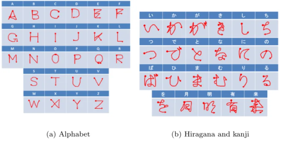
To apply TSCDP, we made a reference model of each character, represented by a single stroke composed of pixels and their location parameters. TSCDP can be applied to two kinds of characters in the air: isolated and connected.

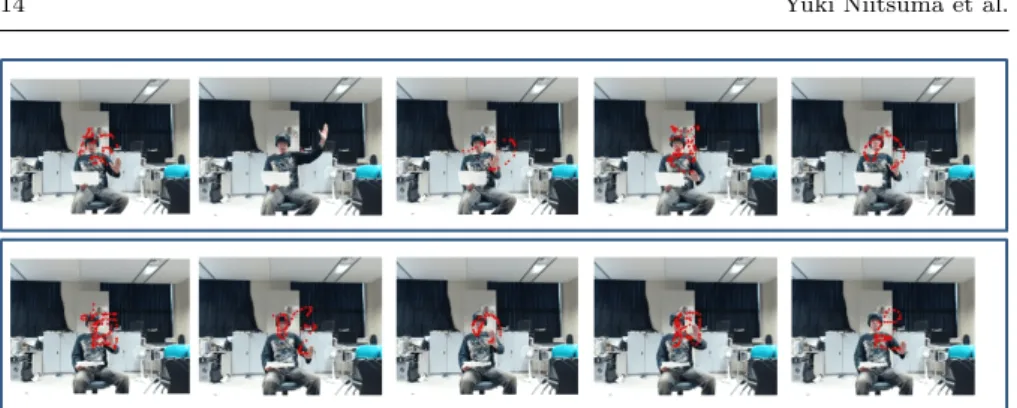
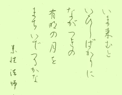
Spotting recognition via TSCDP is better than conventional methods for rec- ognizing connected air-drawn characters. This is because time segmentation is required to separate connected characters into individual characters, and because position variation can be large when connected characters are drawn in the air. We used a video of air-drawn isolated characters, unadorned with tagging data such as start or end times or the location of the characters. To obtain video data on connected characters, we used a work that is famous in Japanese literature (the “Waka of Hyakunin Isshu”), drawn in the air. We made a set of reference point trajectories, each of which represented a single stroke corresponding to an alphabetic, hiragana or kanji character.

2 Related Work

There has been much research on recognizing air-drawn characters. The projects

described below aimed to recognize isolated air-drawn characters, but recog-

nition in a video stream of connected air-drawn characters has not yet been investigated. Okada and Muraoka et al. [3][4][5] proposed a method for ex- tracting the hand area with brightness values, together with the position of the center of the hand, and they evaluated that technique. Horo and Inaba [6] proposed a method for constructing a human model from images captured by multiple cameras and obtaining the barycentric position of this model. By assuming that the fingertip voxels would be furthest from this position, they extracted the trajectory of the fingertips and were then able to recognize char- acters via continuous dynamic programming (CDP) [7]. Florian Baumann et al. proposed a feature called motion binary pattern by combining volume lo- cal binary patterns and optical flow [8] and applied it to the KTH dataset [9]

using histograms of the features. Sato et al. [10] proposed a method that used a time-of-flight camera to obtain distances, extract hand areas, and calculate some characteristic features. They then achieved recognition by comparing the reference features and input features via a hidden Markov model. Nakai and Yonezawa et al. [11][12] proposed a method that used an acceleration sensor (e.g., a Wii remote controller) to obtain a trajectory that was described in terms of eight stroke directions. They then recognized characters via a char- acter dictionary. Scaroff et al. [13][14][15][12] proposed a method for matching time–space patterns using dynamic programming (DP). Their method used a sequence of feature vectors to construct a model of each character. Each fea- ture vector was composed of four elements: the location (x, y) and the motion parameters (v _x , v _y ) (i.e., their mean and variance). Their method therefore requires users to draw characters within a restricted spatial area of a scene.

Moreover, movement in the background or video captured by a moving camera is not accommodated because the motion parameters for the feature vector of the model are strongly affected by any movement in the input video.

These conventional methods (except Ezaki et al. [16], which used an accel- eration sensor) use local features comprising depth, color(*), location param- eters, motion parameters, and so on, to construct each character model. They then applied algorithms, such as DP or a hidden Markov model, to match the models to the input patterns. These methods remain problematic because such local features are not robust when confronted with the severely demand- ing characteristics of the real world. When they are used to recognize air-drawn characters, conventional methods perform poorly if there are occlusions, spa- tial shifting of the characters drawn in the scene, moving backgrounds, or moving images captured by a moving camera.

3 CDP

CDP [7] matches and recognizes a reference temporal sequence pattern in

an unbounded and nonsegmented temporal sequence pattern with allowance

for nonlinear deformation of the reference pattern. Let g(τ ) be a value of

time τ, 1 ≤ τ ≤ T in a reference sequence and let f(t) be a value of time

t, t ∈ ( −∞ , ∞ ) in an input sequence. We define a function for the ith mapping

of each reference and input sequence from t(i) to τ(i) as r(i) = τ (i) | t(i) → τ(i), where i, t(i), and τ(i) are defined as i = 1, 2, . . . , T , t(i) ∈ ( −∞ , t] and τ(i) ∈ [1, T ]. This function r(i) is constructed as a vector of functions r = (r(1), r(2), . . . , r(T )). Hence, the definition of the minimum value of the eval- uation function with local distance d(t, τ) is given by:

D(t, T ) = min

r

∑ T i=1

{ d(t(i), r(i)) } , (1)

where t(1) ≤ t(2) ≤ . . . ≤ t(T) = t. Here, local distance is defined by:

d(t, τ) = || f (t) − g(τ) || . (2)

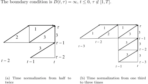
Let a constraint between r(i) and r(i + 1) set three paths, “equal,” “half,”

and “twice,” as shown in Figure 1(a) as determined by the local constraint of CDP for allowing nonlinear deformation of matching. The recursive equation for determining D(t, τ) is:

D(t, τ) = min

 



D(t − 2, τ − 1) + 2d(t − 1, τ ) + d(t, τ );

D(t − 1, τ − 1) + 3d(t, τ);

D(t − 1, τ − 2) + 3d(t, τ − 1) + 3d(t, τ).

(3) The boundary condition is D(t, τ) = ∞ , t ≤ 0, τ ̸∈ [1, T ].

(a) Time normalization from half to twice

(b) Time normalization from one third to three times

Figure 1 Two types of local constraints used in CDP. The number attached to each edge (arrow) indicates the weight of the path.

When accumulating local distances optimally, CDP performs time warping

to allow for variations from half to twice the reference pattern. The selection of

the best local paths is performed by the recursive equation in Eqn. (3). Figure

1 shows two types of local constraints used in CDP for time normalization. In

this paper, we use type (a). Other normalizations, such as from one quarter

to four times, can be realized in a similar way.

4 TSCDP

TSCDP [2] is an extension of CDP that embeds the parameters of the spa- tial axes (x, y) on an image sequence. The main goals of TSCDP are to avoid presegmentation of the input image sequence and to establish nonlinear de- formation and position-free matching. From these three main concepts, this method provides robust recognition of reference patterns. Most conventional recognition schemes have three steps: presegmentation, tracking and match- ing. Thus, these methods have numerous parameters that allow extraction of precise results in each step. Tracking and matching can be applied simulta- neously by a DTW-based method, but require precise presegmentation. The reasons for the success of TSCDP are:

– Segmentation-free design in temporal sequences derived from CDP – Applying relative position constraints in the local distance calculation – Applying relative color distances in the local distance calculation in the accumulation calculation in TSCDP.

The original paper [2] was not optimized to real motion data. Thus, we also provide better implementation for isolated air-drawn characters to improve the recognition rate.

4.1 Evaluation Function for TSCDP

Let f (x, y, t) be a pixel value at position (x, y) of frame t. Here, x, y, and t are limited to 1 ≤ x ≤ M , 1 ≤ y ≤ N, and 1 ≤ t ≤ ∞ , respectively, where M and N are the image width and height in an image sequence. If this image sequence has a gray scale, then f (x, y, t) is a scalar value, but if the image is in color, then f (x, y, t) is a vector that can be derived from any color model.

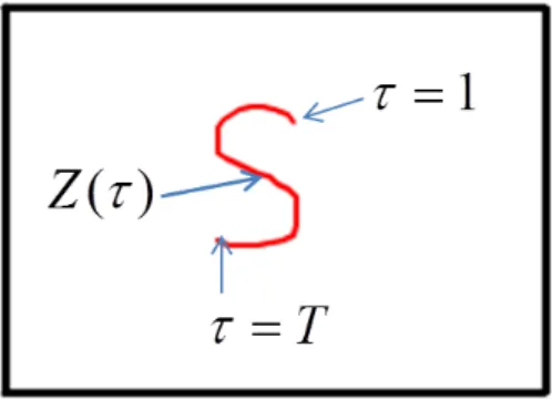
Define a sequence of pixel values for reference pattern Z as:

Z(ξ(τ), η(τ)), τ = 1, 2, . . . , T, (4) where (ξ(τ), η(τ)) is the location in a two-dimensional plane and Z is the pixel with a gray-scale or color value at that location. Here, ξ and η define a reference trajectory (a sequence of spatial positions) of x and y. Next, the local distance between a reference value and the input images is defined by:

d(x, y, τ, t) = ∥ Z(ξ(τ), η(τ)) − f (x, y, t) ∥ . (5) The minimum value of the evaluation function is defined using the following notations:

x(i) ∈ X, y(i) ∈ Y, ξ(i) ∈ X, η(i) ∈ Y, x = x(T ), y = y(T ),

τ(T) = T, t(T ) = t, (6)

a mapping function u i :(ξ(i), η(i)) → (x(i), y(i)),

Here, w = (r, u 1 , u 2 , . . . , u T ) is a vector of functions, where a vector of functions r is defined as for CDP. Finally, the optimization function is defined by:

S(x, y, T, t) = min

w {

∑ T i=1

d(x(i), y(i), τ(i), t(i)) } . (7) Here, the three-dimensional tensor S(x, y, 1, t) is a space of candidate start points for optimal matching: S(x, y, 1, t) = w · d(x, y, 1, t).

Incidentally, the parameters ξ and η are not used explicitly in either the solution algorithm or the local distance for position-free matching. To provide a position-free function for the reference pattern, we set a sequence of difference vectors V (τ) = (v ξ (τ), v η (τ)) as:

v ξ (τ ) = ξ(τ ) − ξ(τ − 1), v η (τ) = η(τ ) − η(τ − 1), (8) where τ = 1, (v ξ (τ ), v η (τ )) = (0, 0) for the boundary conditions.

4.2 Algorithm for TSCDP

When recognizing isolated or connected air-drawn characters, temporal shrink- ing and expansion can occur with spatial shifting. The following formula is the algorithm to determine S(x, y, T, t), by performing time–space warping. The allowable ranges for shrinking and expansion in time and space are each from half to twice the reference point trajectory. Temporal shrinking and expansion from half to twice is realized by the CDP embedded in TSCDP.

4.2.1 Spatiotemporal Deformation Model

We explain the basic mechanism of the local computation of TSCDP. Let the spatial shrinking and expansion be realized by the second minimum calculation of TSCDP, using a parameter A. Here, we define A as A = { ¹ ₂ , 1, 2 } , which allows spatial shrinking and expansion from half to twice the reference pattern.

A allows these deformation patterns by reference vector. The deformation of each local selection is:

A = { 1 2 , 1, 2 } ,

S(x, y, 1, t) = 3d(x, y, 1, t), 2 ≤ τ ≤ T

Then the local distance selection with temporal deformation about t is defined by the following equation derived from the CDP scheme (3):

S(x, y, τ, t) = min

α ∈ A min

 

 

 

 

 

 

 



S(x − α · v _ξ (τ), y − α · v _η (τ), τ − 1, t − 2) + 2d(x, y, τ, t − 1) + d(x, y, τ, t);

S(x − α · v _ξ (τ), y − α · v _η (τ), τ − 1, t − 1) + 3d(x, y, τ, t);

S(x − α · (v ξ (τ ) + v ξ (τ − 1)), y − α · (v η (τ) + v η (τ − 1)), τ − 2, t − 1) + 3d(x − α · v ξ (τ), y − α · v η (τ ), τ − 1, t) + 3d(x, y, τ, t)

(9)

The boundary condition is:

S(x, y, τ, t) = ∞ , d(x, y, τ, t) = ∞ , if (x, y) ̸∈ [M, N ], t ≤ 0, τ ̸∈ [1, T ].

Eqn. (9) is used for the time–space optimization of the evaluation shown by Eqn. (7) as illustrated in Figure 2. The function of the time normalization part of Eqn. (9) is the same as that for CDP. The function of space normalization is simply added to CDP by introducing (x, y)-space to (t, τ) space. Therefore, we consider an algorithm working in a four-dimensional space such as (x, y, t, τ ).

4.2.2 Normalization for Local Deformation in Temporal Domain

The scheme of CDP has three candidate paths for selecting optimal local matching. In general DP matching, the problem is how to realize space nor- malization, and CDP already implements space normalization as shown in Figure 3. TSCDP inherits this scheme. The simplest example of a shrink path shown in Figure 2 corresponds to the third path of Figure 3. Here, the deciding path condition of TSCDP is in the four-dimensional space and it is embedded in two-dimensional space in the temporal space of the CDP scheme. In Figure 2, the t and t − 1 appearing twice in the third path of CDP have three points of τ, namely τ, τ − 1, τ − 2. Therefore, we can consider three points in 4-D space. Then the locations of the (x, y) coordinates of each of the three points have τ parameters, respectively.

We consider that the difference between τ parameters corresponds to a difference in (x, y) of the images in the input video. The difference in the point sequence (x, y) is represented as a difference vector (v ξ , v η ), as shown in Figure 2. This representation was already shown in Egn. (8). Then we embed suitable values of parameters of (v ξ , v η ) into S(x, y, τ, t) and d(x, y, τ, t) of Eqn. (9), but this equation defines only temporal normalization; spatial normalization is embedded as the symbol A.

If the size of (v _ξ , v _η ) is modified, spatial normalization of the reference

pattern can be realized. Now we consider three types of space size modification

at each local optimization, namely { ¹ ₂ , 1, 2 } . This means that any combination

of local spatial size modifications from half to twice the reference pattern

can be realized. This function is realized by introducing the parameters α,

A = { ¹ ₂ , 1, 2 } , and min α ∈ A into the recursive TSCDP equation. The first and

second candidate paths in Eqn. (9) are handled in the same way that the third

candidate path is handled.

Figure 2 Eqn. (9) realizes optimal pixel matching using three candidate paths for time normalization by accumulation of local distances between pixel values of the reference and the input video. The figure shows how the third path works during optimal path selection in 4-D space. The other two paths work in a similar way.

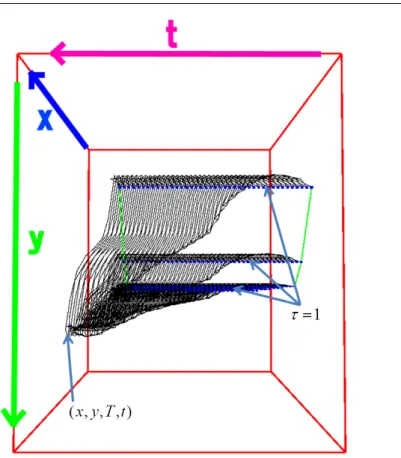
Consider the example reference pattern shown in Figure 3. The allowable time–space search area arrives at the time–space point (x, y, T, t), as shown in Figure 4. TSCDP determines the optimal matching trajectory in this allowable time–space search area. This area is dependent on the reference model for the pixel sequence. In other words, each reference model has its own allowable search area. This differs from conventional DP matching algorithms, which have the same search areas for all reference sequences.

Figure 3 A reference pattern (pixel sequence) made by drawing one stroke sequence (a

sequence of location parameters, ((ξ(τ), η(τ)), τ = 1, 2, ..., T ) on a two-dimensional plane,

where the length of stroke corresponds to T ) of the reference pattern. Each pixel value

Z(ξ(τ), η(τ)) of the reference pattern is assigned a constant skin color.

Figure 4 Search space for TSCDP in arriving at the time–space point (x, y, T , t). Each reference model has its own search space.

4.3 Time-segmentation-free and Position-free Recognition

For the accumulation calculation in TSCDP, we use the recursive equation (9), which is convolved with minimal value selection on temporal and spatial candidates. In other words, S(x, y, 1, t) is a candidate space for a start point and S(x, y, T, t) is a candidate space for a position-free end (spotting) point of matching. Here, the optimal accumulated value S(x, y, T, t) at each time t indicates a two-dimensional scalar field with respect to (x, y). Location (x, y) is called a recognition location if it satisfies the condition S(x, y, T, t) ≤ h.

The recognition location indicates that a category represented by a reference pattern is recognized at time t ∈ [0, T ] and location (x, y). Usually, locations neighboring a recognition location are also recognition locations, because they have similar matching trajectories in the 4-D ((x, y, τ, t)) space. We define such location as the local area of recognition locations.

At each time t, we can find an arbitrary number of local areas of recognition

locations, depending on the number of existing time–space patterns that are

optimally matched with a reference pattern. Then we can determine a location,

denoted by (x ^∗ , y ^∗ ), giving the minimum value of S(x, y, T, t) for each local area of the recognition locations. The number of these locations is the number of recognition locations at time t. A local area of recognition location can be created at an arbitrary position on the (x, y)-plane, depending on the input video. This procedure, which is based on S(x, y, T, t), is the realization of the position-free (spotting) recognition of TSCDP.

On the other hand, a local minimum location (x ^∗ , y ^∗ ) has a time parameter t. If we consider the time series of a local minimum location, we can detect the time duration, denoted by [t _s , t _e ], satisfying S(x ^∗ , y ^∗ , T, t) ≤ h, t ∈ [t _s , t _e ]. The minimum value, denoted by S(x ^∗ , y ^∗ , T, t _reco ), among S(x ^∗ , y ^∗ , T, t), t ∈ [t _s , t _e ], corresponds to the recognition considering time–space axes.

The time t _reco indicates the end time of a recognized pattern in an input query video determined without any segmentation in advance. The starting time of the recognized pattern is determined by back-tracing the matching paths of TSCDP, starting from t _reco . This procedure is the realization of time- segmentation-free (spotting) recognition, based on TSCDP. The following al- gorithms are used in the above procedures. The term [local area] in the follow- ing formulae is the local area of recognition locations, which was used in the above discussion.

(x ^∗ , y ^∗ , T, t) = arg min

(x,y) ∈ [local area] { S(x, y, T, t) } (10) Spotting recognition of multiple categories is determined by using multi- ple reference patterns. Define the ith reference pattern of a pixel series that corresponds to the ith category by:

Z i (ξ(τ), η(τ)), τ = 1, 2, . . . , T i . (11) TSCDP then detects one or more S i (x ^∗ , y ^∗ , T i , t) values as frame-by-frame minimum accumulation values for which ^S

^(x

_3T ^,y

^,T

^,t)

i

≤ h is satisfied. The following equations determine the spotting result for multiple categories:

i ^∗ (t) = arg min

i

S i (x ^∗ , y ^∗ , T, t)

3T _i (12)

S _i (x ^∗ , y ^∗ , T _i , t) = min

(x,y) ∈ [local area]

S _i (x, y, T, t). (13) Figure 5 shows the time-segmentation-free (spotting) recognition of connected cursive air-drawn characters.

5 Constraint-free Characteristics of TSCDP

As mentioned above, most conventional recognition systems are subject to

many technical restrictions such as temporal or spatial segmentation, nonlinear

deformation, color stabilization or discontinuity of patterns. A system based

on TSCDP can dispense with many of these restrictions, as our experimental

Figure 5 Time-segmentation-free recognition for connected characters. Two connected characters are separately recognized at different time points without advance segmentation.

results below indicate. Note that we did not require long-sleeved clothing or colored gloves for color stabilization.

Using a reference pattern composed of pixels with a constant skin color, TSCDP optimally matches only an existing pixel sequence in an input video without identifying any areas of hand or finger. The inferred skin tone is roughly determined without deep investigation, but TSCDP works well us- ing the heuristically derived skin color. Thus, TSCDP seems robust against variations in skin color.

TSCDP is also robust against complex and moving backgrounds because a matched trajectory in TSCDP is only a sequence of pixels (a macroscopic and specified motion with time length T ). Therefore, moving backgrounds, including head or face movement, do not interfere with the total accumulation value of local distances as long as the moving backgrounds are not similar to a reference pattern with a period of around length T . Figure 6 illustrates the recognition of a gesture in a complex and moving background.

TSCDP allows nonlinear variations from half to twice the velocity of move-

ment by the CDP part of TSCDP. Figure 5 illustrates time-segmentation

recognition without any segmentation of start and end times after adapting

nonlinear time variations. Constraints of fixed body location and pose-specific

initial hand location are required by conventional methods because they are

position-dependent when they match a model sequence and a video. The model

for conventional methods is made by features that include location parameters,

so all target matching procedures are still location-dependent. The reference

pattern of TSCDP also has location parameters. However, the dependency on

Figure 6 Recognition of an air-drawn gesture in a complex scene with moving objects in the background. The scene includes people walking in the background, and the static background is a normal office environment.

location is relaxed by directly embedding the location difference u ξ (τ), v η (τ) in the time-warping candidate paths. The position-free characteristic property is then realized in TSCDP, as mentioned in Section 4.3. Allowance for spa- tial shrinking and expansion are also realized by embedding path selection for contracting and dilating spatial size, using both u ξ (τ), v η (τ) and a set of parameters A in the recursive equation of TSCDP. Figure 7 shows a reference pattern that is recognized at different positions when multiple and similar time–space patterns exist in a video.

Figure 7 A reference pattern is recognized at different positions (right and down, left and up), each of which corresponds to a similar trajectory in the video.

TSCDP is also robust when presented with overlapping hands or occlusion

because these cases increase only a relatively small part of the accumulated

value S(x, y, T, t), depending on the spatial and temporal sizes of the overlap-

ping hands or hands over the face or occlusion by objects between the camera

and subject. Figure 8 shows that a gesture is correctly recognized even in

the presence of occlusion. A reference pattern can be made by any kind of

Figure 8 The upper figure shows occlusion occurring at the beginning of drawing the ‘S’

character. The lower figure shows occlusion occurring during the middle period. TSCDP recognizes character gestures correctly in both cases.

single-stroke sequence projected on a two-dimensional plane. Therefore, a ref-

erence pattern with a complex shape and long duration is acceptable. Chinese

kanji characters belong to this category. It becomes even easier to recognize

complex and long reference patterns using TSCDP because they are more dis-

tinguishable from one another. Complex reference patterns allow the use of

a large vocabulary. Figure 9 shows the recognition of complex Chinese char-

acters, including the character “kuru” (“come” in English), which is the last

one in Figure 11(b). A set of gesture patterns caused by various fields of view

of the hand is generated by nonlinear time and space deformations of the

Figure 9 Complex Chinese characters are recognized by TSCDP.

reference pattern. Let { F(x, y) | (x, y) ∈ R } be the image of an object at a fixed time t ₀ , where R is a raster (two-dimension pixel area) and t ≥ t ₀ is a time. Define the distance p(t) [cm] between the camera and the object and parameter c (the value is determined by calibration). If the camera moves p(t) forward or backward relative to the object, then the two-dimensional image of the object shrinks or expands, which in simple geometric terms is described by { F(x × c ^p(t _p(t)

⁾ , y × c ^p(t _p(t)

⁾ ) | (x, y) ∈ R } , where c is a parameter used to transform a value of distance ratio to pixel size. If the conditions of range ^x ₂ ≤ x × c ^p(t _p(t)

⁾ ≤ 2x and ^y ₂ ≤ y × c ^p(t _p(t)

⁾ ≤ 2y are satisfied, the space normalization of TSCDP works well.

On the other hand, let x(t) define the pixel size of the rightward or leftward motion of the camera at time t from x(t 0 ) = 0, where x(t) > 0 for rightward motion and x(t) < 0 for leftward motion, assuming no vertical movement.

Then the two-dimensional image of an object expands in the right or left direction and is described by { F(x + x(t), y) | (x, y) ∈ R } . If the condition of range ^x ₂ ≤ x(t) ≤ 2x is satisfied, then the space normalization of TSCDP works well.

Let F(t) be the image of an object at t with a combination of two kinds of camera motion. Then F (t) is determined by

F (t) = { F ((x + x(t) } ) × c p(t ₀ )

p(t) , y × c p(t ₀ )

p(t) ) | (x, y) ∈ R } .

If the conditions of the range, ^x ₂ ≤ (x+x(t) } ) × c _p(t) ^p

≤ 2x and ^y ₂ ≤ y × c ^p(t _p(t)

⁾ ≤ 2y, are satisfied, the space normalization of TSCDP works well.

If time shrinkage or expansion occurs as a side effect of camera motion, time normalization of TSCDP works well, scaling from half to twice the size.

This reasoning is equivalent to the claim that if a pixel trajectory is included in F (t), (t ∈ [t 0 , t]) and also belongs to the time–space area of Figure 5 of a reference pattern, then the pixel trajectory is well recognized by TSCDP.

Otherwise, the accumulated local distance S increases, depending on the size

of the part of the trajectory outside the time–space area of Figure 5. If the

increased accumulated distance S is smaller than threshold h, then the tra-

jectory is recognized. If we set a higher threshold value h, the recognition system becomes more robust against greatly deformed input patterns at the cost of increasing the error rate. Robustness and error rate are a trade-off in determining the threshold value h.

Figure 10 shows that the continuously deforming image of a gesture is well recognized in a video that captures the gesture while the distance from and orientation to the camera change.

6 Modeling Reference Patterns

The first step in recognizing air-drawn characters via TSCDP is to make a model of each character’s category, as a reference pattern for TSCDP. This TSCDP reference pattern (model) is determined by the stream of pixels form- ing a trajectory on a two-dimensional plane. This procedure corresponds to the learning procedure for making a model used in conventional on- or offline char- acter recognition. However, our method is different from conventional learn- ing methods. We do not use sample videos for making reference patterns in TSCDP. A reference pattern in TSCDP is made by air-drawing one stroke pro- jected on a two-dimensional plane. A stroke is a sequence of parameters of pixel location ξ(τ), η(τ), τ = 1, 2, ..., T . The length of a stroke corresponds to T . Each location of the stroke is assigned a pixel value, denoted by Z(ξ(τ), η(τ)), expressing a constant skin color. Finally, the reference pattern is represented by Z(ξ(τ), η(τ)), τ = 1, 2, ..., T . The second step is the treatment of the single- stroke representation of a model. The stream is composed of connected straight or curved lines. Categories for characters such as ‘C,’ ‘O’ and ‘Q’ are used to represent a one-stroke model. However, most other characters, including those from the alphabet or Japanese hiragana or kanji characters, cannot be drawn as a single stroke. In this case, we make a one-stroke model for each character by connecting its separate strokes with additional strokes in the air. These additional strokes are not part of the actual strokes in the character. By us- ing this kind of modeling for each character, TSCDP can be adapted for its recognition.

We prepared single-stroke models of each category of alphabetic and of

Japanese hiragana and kanji characters. The input pattern is obtained from

a video capturing isolated characters or a sequence of connected cursive char-

acters drawn by a human hand in the air. We do not specify the start and

end times of each drawing, even for isolated characters. Furthermore, a color

finger cap, gloves, or any special device are required. Applying TSCDP to a

character model with category number i, we obtain i ^∗ (t), where the time t is

called the spotting time.

(a) Starting image of the moving camera.

(b) Ending image of the moving camera.

Figure 10 A moving camera captures a gesture deformed by changing distance and orien-

tation to the camera. TSCDP can recognize the deformed gesture.

7 Experiments

7.1 Database and Performance in a Comparison Study

We used videos obtained by capturing air-drawn gestures and characters made with one stroke in a position-free style. Some of these gesture videos include large occlusions, multiple gestures in a single scene, or connected characters.

Some were captured by a moving camera with moving backgrounds. No previ- ous experiment applied conventional methods to real data. Therefore, it seems impossible to compare our method with the conventional methods described in previous studies [3][6][8][9][10][11]. Moreover, our database is rather small.

Therefore, the experiments reported here are regarded as preliminary trials to investigate whether or not TSCDP can relax the many constraints mentioned in the introduction, before its application to a large amount of real-world data.

To recognize air-drawn characters, we apply two kinds of spotting recognitions using the same TSCDP. The final algorithms differ from each other, as men- tioned in Section 4.

7.2 Experimental Conditions

Figure 11(a) shows a set of reference patterns for an alphabet of 26 categories, each of which is a one-stroke model. In addition, we manually constructed a set

(a) Alphabet (b) Hiragana and kanji

Figure 11 List of reference patterns. Each reference pattern is made with a single stroke.

of one-stroke characters, as seen in Figure 11(b). These one-stroke characters

are used in the Waka poem and are regarded as the reference patterns when

applying TSCDP in parallel. Figure 12 shows a sheet of paper upon which the

famous Japanese “Waka Imakomuto” from the “Hyakunin Isshu” is written.

We showed this example to the participants, who were instructed to write the Waka in the air using connected characters. The experimental conditions were

Figure 12 An example of “Waka” is shown to each person and is used to draw a sequence of connected cursive characters in the air.

as follows:

– Video:

– Frames per second: 20 fps – Resolution: 200 × 150 pixels

– RGB color was used (8 bits per color) – Reference patterns for characters:

– A single-stroke reference pattern was constructed manually for each character.

– A spatial distance of 3 pixels along a stroke in the plane (ξ, η) corre- sponding to 50 ms in parameter τ of Z. These parameters were fixed for all reference patterns. The total length L pixels of each stroke de- termined T = (L/3) × 50 ms in Z.

– Scene:

– Each person wrote isolated characters in the air without specific start or end times. They also wrote connected characters in the air, column by column, without a specific start or end time.

– Three participants drew the characters.

– The list of hiragana and kanji models (26 alphabetic characters) for recog-

nizing isolated characters is shown in Figure 11(a).

– The list of models (23 references) for recognizing connected characters is shown in Figure 11(b). The writing style for connected cursive characters (Figure 12) was shown to each participant in advance.

– Parameters:

– The spotting recognition threshold was h = 15 (fixed).

– Z = (R, G, B) = (190, 145, 145) (fixed).

– The Euclidian norm was used for calculating local distance.

7.3 Two Kinds of Determination Methods

Recognition is basically carried out using spotting points of TSCDP values.

We use two determination methods to obtain the recognition results: unique determination and candidate-ranking determination. The former uses the best candidate, while the latter uses candidates from best to kth. In our experi- ments, only the former method is used for the recognition of connected char- acters. Both methods are used for the isolated air-drawn characters. If we use contextual information provided by a dictionary to correct errors in the post-processing stage, ranking of multiple candidates is more useful.

7.3.1 Three Kinds of Threshold Values

TSCDP uses a spotting threshold to determine the time–space spotting point.

First, we determine a single and common threshold called the first type of threshold value, which applies to all categories. However, each accumulated value represented by S(x, y, T, t) varies depending on the reference pattern, even if it is normalized by 3T .

Furthermore, we determined that the thresholds should be adapted to each category.

Both the velocities of manually drawing a reference pattern and the tra- jectory extracted from the input video are essential to determine the optimal threshold. The adaptation is to multiply the parameter value by the prefixed optimal threshold. The parameter value is determined by:

V _ref (distance/f rame) : V elocity of ref erence pattern,

V in (distance/f rame) : V elocity of input pattern (backtrack trajectory),

M = V in / V ref . (14)

The optimal threshold is determined by:

n : N umber of experimental persons, h o = ( 1

n

∑ n i=1

S T (X)) × M. (15)

In each reference pattern, each optimal threshold is denoted by h o (i) as the

second type of threshold value. We use another threshold value, which is called

Figure 13 The list of optimal thresholds and the upper limit threshold for alphabet cat- egories. The optimal threshold for category “X” is not the average value because person C gives an outlier.

the upper limit threshold value. When a category’s accumulated value of spot- ting points exceeds the upper limit value, we have no output at time t.

The upper limit threshold is determined by:

h upper = max

i ∈ n (S i (x, y, T i , t)) × B. (16) We call this the third type of threshold value. The parameter B was experi- mentally determined as B = 1.2.

The optimal and the upper limit thresholds are shown in Figure 13. The optimal threshold value was experimentally determined as n = 3.

7.3.2 Unique Determination Using Maximum Stroke

As mentioned in Section 4.1, each category i has the accumulated value S i (x, y, T, t)

at t and arg min _{(x,y) ∈ [local area],t ∈ [t}

_,t

_] S i (x, y, T, t) ≤ 3T i × h gives a spot-

ting time–space point (x ^∗ , y ^∗ , t ^∗ ), where h is a single and common threshold

value, and h = 15 was experimentally determined. For a category i, we can

Figure 14 Use of two different optimal threshold values for determining a candidate rank- ing.

obtain a i ^∗ (t) if there is a spotting point. Among multiple i ^∗ (t) values, the recognition output for time t is uniquely determined by selecting the category with the maximum stroke length. We called this method unique determina- tion for recognition. At present, there is no theoretical reason to choose the maximum stroke length as a criterion. It was observed that a longer stroke reference had a greater tendency to accumulate local distances than a shorter stroke. This is not normalized by the normalizing parameter 3T

7.3.3 Candidate Ranking Determination

In handwritten character recognition, a set of recognition candidates is pre- pared to identify contexts in a word dictionary to obtain a higher recognition score. We take account of candidate rankings for further use in the post- processing of TSCDP. We calculate the so-called ranking distance. Let X denote the input video and Y the reference pattern and apply TSCDP. By subtracting the accumulation value, S(x ^∗ , y ∗ , T, t), from the optimal thresh- old, the ranking distance D(X, Y ) is determined by:

S T (X ) : Accumulated V alue on X h o (Y ) : U pper limit T hreshold on Y

D(X, Y ) = h o (Y ) − S T (X ). (17)

We obtain a set of ranking distances and sort them for ranking.

Figure 14 shows how two different optimal thresholds are used for deter- mining the candidate ranking.

7.4 Isolated Character Recognition

When we use unique determination to recognize isolated characters, we con-

sider two types of errors: confusion and missing. A confusion error designates

incorrect recognition output. A missing error means that there is no output because the accumulated value of the spotting point exceeds the common threshold value (h = 15). The recognition rates are shown in Table 1.

Table 1 Results for isolated characters using unique determination.

Result Total Person A Person B Person C

Correct 65.4% 46.2% 69.2% 80.8%

Missing 5.1% 0.0% 3.8% 11.5%

Confusion 29.5% 53.8% 26.9% 7.7%

Figure 15 shows the confusion matrix for the recognition of isolated char- acters. Next, we show a recognition result using candidate ranking determina- tion. The results of all categories are shown in Figure 17. The accumulated ranking is shown in Table 2.

Table 2 Accumulated ranking of candidates for isolated characters.

Best Until Until Until Until

Candidate First Second Third Fourth Fifth All Person A 53.8% 76.9% 76.9% 84.6% 92.3% 92.3%

Person B 34.6% 65.4% 73.1% 76.9% 80.7% 88.5%

Person C 46.1% 65.4% 69.2% 69.2% 73.1% 73.1%

The scores accumulated from the best five candidates by unique determi- nation are shown in Table 3. This table indicates that the recognition score by

Table 3 Comparison between unique determination and unique determination using can- didate ranking for isolated characters.

Accumulation of Unique determination Candidate Best one five candidates using ranking

Person A 53.8% 92.3% 46.2%

Person B 34.6% 80.7% 69.2%

Person C 46.1% 73.1% 80.8%

unique determination was higher if it was combined with information about candidate ranking.

7.5 Connected Character Recognition

For the recognition of connected characters by TSCDP, we adopted only

unique determination. There were three types of errors. The first, “missing

Figure 15 Confusion matrix of recognition results for isolated characters.

(M)”, means that no category was detected at the correct time. The second,

“ghost (G)”, means that an output appeared at an incorrect time. The third,

“confusion (F)”, means that a category was detected at the correct time but it was incorrect. Correct output, that is, “correct (C)”, means that correct out- put was obtained at the correct time. We can then determine each recognition rate as follows.

– Correct rate = C

(M + G + F + C) × 100%

– Missing rate = M

(M + G + F + C) × 100%

– Ghost rate = G

(M + G + F + C) × 100%

(a) Results for participant A

(b) Results for participant B

Figure 16 Alphabet recognition ranking (Participants A and B). The left column indicates

inputs, and the row indicates output candidates from the first to the 12th positions.

(a) Results for participant C

Figure 17 Alphabet recognition ranking (Participant C). The left column indicates inputs, and the row indicates output candidates from the first to the 12th positions.

– Confusion rate = F

(M + G + F + C) × 100%

The recognition rates are shown in Table 4, where Ghost rate = 0%. The confusion matrix is shown in Figure 18.

Table 4 Results for connected characters using unique determination.

Result Total Person A Person B Person C

Correct 64.4% 82.8% 62.1% 48.3%

Missing 11.1% 3.4% 17.2% 13.8%

Confusion 24.5% 13.8% 20.7% 37.9%

8 Conclusion

This study confirmed that TSCDP worked well in recognizing both isolated and connected cursive air-drawn characters in a video. In particular, connected air-drawn characters were recognized without time segmentation in advance.

Moreover, we presented several experimental results for gesture recognition,

Figure 18 Confusion matrix of recognition results for connected alphabetic hiragana and kanji characters.

which demonstrated how TSCDP is free from many constraints, including po- sition restrictions, that are imposed by conventional methods. In our experi- ments, we did not use a large number of videos to capture air-drawn characters.

Therefore, the main objective of this paper was to conduct a feasibility study to determine how TSCDP works to recognize human motions performed under almost no constraints by persons in the real world.

References

1. S.C.W. Ong, S. Ranganath, Pattern Analysis and Machine Intelligence 27(6), 873 (2005)

2. R. Oka, T. Matsuzaki, Joint Technical Meeting on Information Processing and Innova- tive Industrial Systems 27(6), 873 (2012)

3. T. Okada, Y. Muraoka, Transactions of the Institute of Electronics, Information and Communication Engineers D-II J86-D-II(7), 1015 (2003)

4. M. Kolsch, M. Turk, In Proc. Sixth IEEE International Conference on Automatic Face

and Gesture Recognition pp. 614–619 (2004)

5. M. Yang, N. Ahuja, M. Tabb, Pattern Analysis and Machine Intelligence 24(8), 1061 (2002)

6. T. Horo, M. Inaba, Workshop on Interactive Systems and Software (WISS2006) (2006) 7. R. Oka, The Computer Journal 41(8), 559 (1998)

8. F. Baumann, J. Liao, A. Ehlers, B. Rosenhahn, in 3rd International Conference on Pattern Recognition Applications and Methods (2014)

9. I. Laptev, Local spatio-temporal image features for motion interpretation. Ph.D. the- sis, Computational Vision and Active Perception laboratory (CVAP), NADA, KTH, Stockholm (2004)

10. A. Sato, K. Shinoda, S. Furui, Meeting on Image Recognition and Understanding IS3–

44, 1861 (2010)

11. M. Nakai, H. Yonezawa, Forum on Information Technology H–19, 133 (2009) 12. W. Gao, J. Ma, J.Wu, C. Wang, International Journal of Pattern Recognition and

Artificial Intelligence 14(5), 587 (2000)

13. S. Sclaroff, M. Betke, G. Kollios, J. Alon, V. Athitsos, R. Li, J. Magee, T.P. Tian, ICDAR: Int. Conf. on Document Analysis and Recognition (2005)

14. J. Alon, Spatiotemporal gesture segmentation. Dissertation for Doctor of Philosophy, Boston University (2006)

15. F. Chen, C. Fu, C. Huang., Image and Video Computing 21(8), 745 (2003)

16. N. Ezaki, M. Sugimoto, K. Kiyota, S. Yamamoto, Meeting on Image Recognition and

Understanding IS2–48, 1094 (2010)