|||||||||||||||||| Performance Improvements of Multi-hop Ad Hoc Wireless Networks in Distributed Cooperative systems ||||||||||||||||||

(1)

Performance Improvements of Multi-hop Ad Hoc Wireless Networks in Distributed

Cooperative systems

——————————————————

愛知県立大学大学院情報科学研究科博士後期課程

2017841001

真田拓実

指導教員主査田学軍准教授副査村上和人教授副査奥田隆史教授

提出日

:

平成

30

年

12

月

(2)

1 Introduction 1

1.1 Abstract . . . 1

1.2 Construction of the thesis . . . 2

2 Conventional wireless communication systems 5 2.1 IEEE 802.11 standards . . . 5

2.2 IEEE 802.11 architecture . . . 5

2.3 DCF . . . 6

2.4 EDCA . . . 7

2.5 Multi-hop wireless networks . . . 8

2.5.1 Sensing area . . . 9

2.5.2 Hidden node problem . . . 9

2.5.3 Exposed node problem . . . 10

2.5.4 Receiver blocking problem . . . 11

3 Improving the throughput and the fairness in single-hop 13 3.1 Background . . . 14

3.2 Problems of the conventional method . . . 15

3.3 Related works . . . 16

3.4 Analysis and the proposal of optimizing backoﬀ by dynamically estimating the number of nodes . . . 18

3.4.1 Motivation . . . 18

3.4.2 Analytical Study . . . 19

3.4.3 OBEN Scheme . . . 22

3.5 Performance evaluations . . . 24

3.5.1 Throughput . . . 25

3.5.2 Variation of CW and Fairness . . . 27

3.6 Conclusions . . . 28

4 Improving the throughput and the fairness in single-hop with QoS 31 4.1 Problems of the conventional method . . . 31

(3)

cally estimating number of nodes . . . 32

4.3.1 Optimal Backoﬀ . . . 33

4.3.2 Enhancement of QoS . . . 34

4.3.3 OBQ Scheme . . . 35

4.4.1 Estimating number of nodes . . . 37

4.4.2 Throughput . . . 38

4.4.3 Delay . . . 39

4.4.4 Data Dropped . . . 40

4.4.5 Fairness . . . 41

4.4.6 Eﬀect of Traﬃc Configuration . . . 42

5 5. Improving the throughput and the fairness in multi-hop 49 5.1 Problems of the conventional method . . . 49

5.3 Analysis and the proposal of optimizing backoﬀ by dynamically estimating number of nodes . . . 50

5.3.1 Optimal backoﬀ . . . 50

5.3.2 Analysis of Throughput in Multi-hop Networks . . . . 51

5.3.3 Optimal Backoﬀ . . . 54

5.3.4 OBEM Scheme . . . 57

5.4.1 Estimated number of neighbor nodes and hidden nodes 60 5.4.2 Throughput . . . 61

5.4.3 Fairness index . . . 62

6 Conclusions 65 6.1 Conclusions . . . 65

6.2 Future work . . . 66

Acknowledgements 69

Author published paper 71

References 73

(4)

2.1 BSS . . . 6

2.2 IBSS . . . 6

2.3 RTS/CTS/DATA/ACK mechanism . . . 8

2.4 Hidden node problem . . . 10

2.5 The hidden node range . . . 10

2.6 The exposed node problem . . . 11

2.7 The receiver blocking problem . . . 12

3.1 The monthly average mobile communication traﬃc in Japan . 14 3.2 IoT connected devices installed base worldwide from 2015 to 2025 . . . 15

3.3 Monotone function fidl(n) when the real value of n is 50 . . . 17

3.4 The variation of theCW . . . 18

3.5 Monotone function f_idl(n) when the real value of n is 50 . . . 21

3.6 Throughput with average idle slot interval . . . 23

3.7 CW sizes with simulation time when the β is changed . . . . 24

3.8 Throughput with node numbers . . . 26

3.9 CW sizes of a node with simulation time . . . 28

3.10 CW sizes and retransmission attempts of a node with simulation time . . . 29

3.11 Fairness Index . . . 29

4.1 Throughput vs. average idle interval. . . 34

4.2 Estimated number of nodes vs. simulation time. . . 38

4.3 Total throughput of OBQ and IEEE 802.11e with diﬀerent packet size. . . 40

4.4 Total throughput of OBQ and IEEE 802.11e with diﬀerent packet size. . . 41

4.5 Total throughput vs. oﬀered load when the CW ratio is changed. . . 42

4.6 Maximum total throughput with diﬀerent frame lengths. . . . 42

4.7 Total throughput vs. oﬀered load when the background noise varies. . . 43

(5)

4.9 Delay and throughput of AC[VO] and AC[VI] vs. oﬀered load. 44

4.10 Delay and throughput of AC[BE] vs. oﬀered load. . . 45

4.11 Delay of AC[VO] and AC[VI] vs. oﬀered load when theCW ratio is changed. . . 45

4.12 Delay of AC[BE] vs. oﬀered traﬃc when the CW ratio is changed. . . 46

4.13 Data dropped vs. oﬀered traﬃc when theCW ratio is changed. 46 4.14 Fairness index when the CW ratio is changed. . . 47

4.15 Throughput of each AC vs. oﬀered load when the traﬃc configuration is changed. . . 47

4.16 Delay of AC[VO] vs. oﬀered load when the traﬃc configuration is changed. . . 48

5.1 Classification of each node . . . 52

5.2 The f_idl(n) when the real value of nis 50 . . . 56

5.3 Throughput with average idle interval when the ratio ofnto h(r) is changed . . . . 57

5.4 Throughput with average idle interval when the ratio ofnto h(r) are 0.1 and 0.5 . . . 58

5.5 A snapshot of nodes distribution in simulation . . . 61

5.6 Estimated number of neighbor nodes and hidden nodes with simulation time . . . 62

5.7 Throughput with a diﬀerent ratio of n to h(r) . . . 63

5.8 Throughput with a diﬀerent payload size . . . 64

5.9 Fairness index . . . 64

6.1 Application of the proposed method OBEN in vehicle to vehicle communication . . . 67

6.2 Application of the proposed method OBQ in vehicle to vehicle communication . . . 68

6.3 Application of the proposed method OBEM in vehicle to vehicle communication . . . 68

(6)

2.1 List of IEEE 802.11 standards . . . 6

2.2 Each AC priority . . . 8

2.3 Path loss exponent . . . 9

3.1 Access method in IEEE 802.11 . . . 16

3.2 Network configuration . . . 25

3.3 Backoﬀ parameters . . . 25

3.4 Throughput (Kbps) with node numbers . . . 26

5.1 The probabilities of each node state . . . 54

(7)

(8)

Introduction

1.1 Abstract

Wireless local area networks(WLANs) have become increasingly popular and widely deployed. Since all the nodes share a common wireless channel with limited bandwidth in WLANs, it is highly desirable that an eﬃcient and fair medium access control(MAC) protocol is employed. The fundamental access method of the IEEE802.11 (The Institute of Electrical and Electronics Engineers) MAC is a DCF (Distributed Coordination Function) and an optional centralized one called Point Coordination Function(PCF).

Due to its inherent simplicity and flexibility, the DCF is preferred in the case of no base station such as vehicle to vehicle communications. In DCF, there are three problems as follows. First, the throughput decreases when the number of nodes increases. Second, The variation of the Contention Window(CW) is large, which means that the fairness decreases. Finally, QoS is not guaranteed enough. To improve QoS(Quality of service) in DCF, the IEEE 802.11e has defined EDCA(Enhanced Distributed Channel Ac- cess). Specifically, the throughput and the fairness decrease sharply as the number of nodes increase in EDCA or multi-hop network.

The focus of this thesis is on DCF and EDCA assuming the vehicle to vehicle communications. In vehicle to vehicle communications, each node can reach or leave the network freely. When much nodes enter network, the throughput and fairness decreases sharply. To deploy a flexible and eﬃcient network, the above problems need to be resolved. Thus, this thesis presents the MAC protocols to resolve the above problems through 3 steps.

First, I propose a new novel MAC protocol OBEN (Optimizing Backoﬀ by dynamically Estimating Number of Nodes). OBEN assumes the single- hop network with DCF. In OBEN, each node can estimate the number of nodes, obtain the optimal CW and achieve the high throughput and good fairness. Second, I propose OBQ (Optimizing Backoﬀ with better QoS).

OBQ is based on OBEN and takes QoS into account. OBQ also can achieve

(9)

requirement, each node sets CW for each AC separately, which leads to better QoS. Finally, I propose OBEM(Optimizing Backoﬀ by dynamically Estimating the number of nodes in Multi-hop networks). OBEM expands OBEN in multi-hop wireless networks. In multi-hop wireless networks, the throughput decreases heavily under a high traﬃc load due to the hidden node problem. OBEM can alleviate the hidden node problem and enhance the throughput and the fairness. Through simulations comparison with the conventional method, this thesis shows that OBEN, OBQ and OBEM can greatly enhance the throughput.

1.2 Construction of the thesis

The remainder of this thesis is organized as follows. The Chapter 2 explains the conventional method, DCF and EDCA. The IEEE 802.11 DCF and EDCA are based on a mechanism called carrier sense multiple access with collision avoidance(CSMA/CA). A node with a packet to transmit initializes a backoff timer with a random value selected uniformly from the range [0, CW], where CW is the contention window in terms of time slots. After a node senses that the channel is idle, it begins to decrease the backoff timer by one for each idle time slot. When the channel becomes busy due to other node’s transmissions, the node freezes its backoff timer. When the backoff timer reaches zero, the node begins to transmit. If the transmission is successful, the transmitter resets itsCW toCW_min. In the case of collision, it doubles itsCW until reaching a maximum valueCWmax. The transmitter chooses a new backoff timer and starts the above process again. Also, this chapter introduces the problems characteristic of multi-hop wireless network.

Specifically, those problems are the hidden node problem, exposed node problem and receiver blocking problem. For the throughput analysis in multi-hop wireless network, those problems are important factors.

In Chapter 3, I propose a MAC protocol OBEN, which can improve the throughput and the fairness in single-hop wireless network. In DCF, each node performs the carrier sense and transmits a packet after random wait time. For this random wait time, when the number of nodes increases, the collision is occurred and the throughput decreases. Also, CW is the value related to the node s packet transmission probability, a smallCW results in a high collision probability, whereas a largeCW results in wasted idle time slots and throughput decreases. Because the variation of CW is large in the conventional method DCF, there are problems that the throughput and the fairness are low. To resolve the above problems, I propose a new MAC protocol OBEN. In OBEN, firstly, each node listens to the wireless channel.

The wireless channel events can be thought of as three types of events, successful transmission, collision and idle. Each node observes the three chan-

(10)

nel events, computes the probabilities of each channel events and estimates the number of nodes. Second, based on the number of estimated nodes, each node obtains the optimalCW to achieve high throughput. Therefore, each node dynamically estimates the number of nodes, obtains the optimal CW according to the number of estimated nodes, OBEN achieve the high throughput and the good fairness. Through simulation comparison with the conventional method DCF and the recently proposed methods, this chapter shows that our scheme can greatly enhance the throughput with good fairness.

In Chapter 4, I propose a MAC protocol OBQ, which can be improve the throughput and the fairness in single-hop wireless network with QoS.

IEEE 802.11e has defined the access method EDCA which expands DCF and supports QoS for traffics with different priorities. In EDCA, in addition to the problems of the conventional method DCF, there is a problem that QoS is not guaranteed enough. The node has four AC(Access Category) with different priorities. The high priority AC transmits with priority and needs to act as the high guarantee of successful transmission. However, since the ranges of theCW of the high priority AC is narrow, QoS becomes low in the case of the number of nodes increasing. The proposal method OBQ is a new MAC protocol that is based on OBEN and resolves the above problems. In OBQ, based on OBEN, each node estimates the number of nodes through observing the wireless channel. Based on the number of estimated nodes, each node obtains the optimal CW. With the optimal CW and the transmission opportunity of each AC, CW is set to each AC.

OBQ controls the transmission opportunity of each AC in a node freely according to QoS requirement. The delay of each AC is changed depending on the transmission opportunity of each AC but the total throughput of ACs is not changed. Through simulation comparison with the conventional method DCF, OBQ always maintain the high throughput and provide the satisfied QoS.

In Chapter 5, I propose a MAC protocol OBEM, which can be improve the throughput and the fairness in multi-hop wireless network. OBEN and OBQ assume that the network is in single-hop wireless network, which all nodes are in the communication range. In multi-hop wireless network, the throughput sharply decreases as compared to single-hop when the number of nodes increases. One of the factors is the hidden node problem. RTS/CTS mechanism, which is defined in IEEE 802.11, is used to alleviate the hidden node problem but not enough. Also, because the analysis in multi-hop wireless network becomes complicated by the hidden node problem, the optimalCW according to the number of nodes was not suﬃciently studied.

Due to this, this chapter proposes a new MAC protocol OBEM. OBEM is based on OBEN and applied in multi-hop wireless network. In OBEM, each node observes the wireless channel and computes the probabilities of each wireless channel. Each node estimates the number of neighbor nodes

(11)

and then obtains the optimal CW. Through simulation comparison with the conventional method DCF, this chapter shows that OBEM achieves the high throughput and good fairness.

Finally, the Chapter 6 comprehensively summarizes the results of the research and arrange for future tasks. First, I propose a distributed MAC protocol OBEN. OBEN can estimate the number of nodes dynamically, obtain the optimal CW and then achieve the high throughput and good fairness. Even if the number of nodes is changed, OBEN can adjust the optimalCW dynamically and obtain better performance than the conventional method DCF and the recently proposed methods. Second, based on OBEN, I propose a distributed MAC protocol OBQ. Using the number of estimated nodes, each node obtains the optimal CW. With the optimal CW and the transmission opportunity of each AC, the CW of each AC is set. OBQ control the transmission opportunity of each AC in a node freely according to QoS requirement. The delay of each AC is changed depending on the transmission opportunity of each AC but the total throughput of ACs is not changed. Finally, for the method that adapts to a wider wireless network, I propose a distributed MAC protocol OBEM. Each node dynamically estimates the number of neighbor nodes and hidden nodes, adjust the optimalCW and then alleviate the hidden node problem. Based on detail analysis and simulation results, the proposal MAC protocol achieves high throughput, good fairness, satisfied QoS and adapting to multi-hop wireless network. Thus, it can be established as a communication technology adapted to distributed wireless networks such as vehicle to vehicle communications.

(12)

Conventional wireless communication systems

2.1 IEEE 802.11 standards

IEEE 802.11 standards defined the specific rules for WLANs communication in 1997 [1]. In first generation technology, the maximum throughput of IEEE 802.11 was 2Mbps. IEEE 802.11 was quickly improved and made by IEEE 802.11a and IEEE 802.11b in 1999. IEEE 802.11a operated in 5GHz bands and maximum throughput is 54Mbps. IEEE 802.11b operated in 2.4GHz bands and maximum throughput is 11Mbps. After IEEE 802.11a and IEEE 802.11b, WLANs technologies have improve every year and new standards have been defined as shown in Table 5.1. IEEE 802.11g was defined in 2003 and replaced the older IEEE 802.11b. Subsequently, IEEE 802.11g was replaced by IEEE 802.11n and newer standard. IEEE 802.11n supports four spatial streams 4×4 MIMO (Multiple Input Multiple Output) and a band width of 40MHz. On the other hand, the newer IEEE 802.11ac supports eight spatial streams 8×8 MIMO and a band width of 80MHz, which can be combined to make 160MHz. Moreover, IEEE 802.11ac supports 256-QAM modulation, while IEEE 802.11n supports up from 64-QAM. With such a huge diﬀerence, maximum throughput of IEEE 802.11ac is 7Gbps. In this way, the WLANs technologies have improved and the maximum throughput have increased.

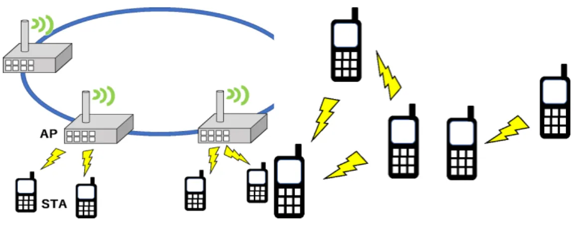
2.2 IEEE 802.11 architecture

The IEEE 802.11 architecture contains several service set: the basic service set (BSS) and the independent BSS (IBSS). The BSS is a wireless network which consists of a single wireless access point (AP) supporting one or multiple wireless stations (STAs), as shown in Fig 2.1. The IBSS is a wilreless network which consists of multiple STAs, as shown in Fig 2.2. BSS is lower

(13)

Table 2.1: List of IEEE 802.11 standards

IEEE 802.11 standard Establishment year band maximum throughput

IEEE 802.11 1997 2.4GHz 2Mbps

IEEE 802.11a 1999 5GHz 54Mbps

IEEE 802.11b 1999 2.4GHz 11Mbps

IEEE 802.11g 2003 2.4GHz 54Mbps

IEEE 802.11n 2009 2.4/5GHz 600Mbps

IEEE 802.11ac 2013 5GHz 7Gbps

collisions than IBSS due to the STAs are controlled by a AP in BSS. Hence, the throughput of BSS is higher than that of IBSS in saturated network.

On the other hand, IBSS can communicate each other without AP, which means that a wireless network can be constructed at low cost. This thesis focuses on IBSS.

Figure 2.1: BSS Figure 2.2: IBSS

2.3 DCF

In IEEE 802.11, the Distributed Coordination Function (DCF) and the Point Coordination Function (PCF) is defined. DCF is the fundamental access method and used in BSS and IBSS. DCF is a random access scheme, which is based on the carrier sense multiple access with collision avoidance (CS- MA/CA). The waiting duration for packet transmission is calculated with the binary exponential backoﬀ algorithm. On the other hand, PCF is an optional centralized scheme which is only used in BSS. In PCF, the AP operate the STAs and entitle the STA to transmit packets. Due to this, the collision is not occurred in PCF. However, in DCF, there is not a operator for packet transmission, which is occurred many collisions. This thesis focuses on DCF

(14)

and explain in detail about DCF as the following.

The DCF is based on a mechanism called carrier sense multiple access with collision avoidance (CSMA/CA). In DCF, a node with a packet to transmit initializes a backoff timer with a random value selected uniformly from the range [0, CW], where CW is the contention window in terms of time slots. After a node senses that the channel is idle for an interval called DIFS (DCF inter-frame space), it begins to decrease the backoff timer by one for each idle time slot. When the channel becomes busy due to other node’s transmissions, the node freezes its backoff timer until the channel is sensed idle for DIFS. When the backoff timer reaches zero, the node begins to transmit. If the transmission is successful, the receiver sends back an acknowledgment (ACK) after an interval called SIFS (short inter- frame space). Then, the transmitter resets its CW to CW_min. In the case of collision, the transmitter fails to receive the ACK from its intended receiver within a specified period, with the result that it doubles itsCW until reaching a maximum value CW_max after an interval called EIFS (extended inter-frame space). The transmitter chooses a new backoff timer and starts the above process again. When the transmission of a packet fails for a maximum number of times, the packet is dropped.

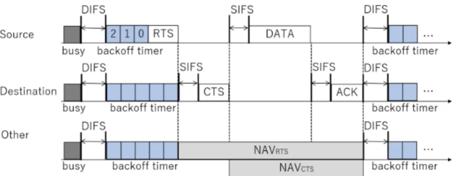
For decreasing the collision and alleviating the hidden node problem (explains in Section 2.5.2), RTS/CTS (Request To Send/Clear To Send) mechanism is used [2]. The Fig. 2.3 shows the RTS/CTS/DATA/ACK mechanism. The source transmits the RTS packet before data transmission.

The destination sends back the CTS packet after receiving the RTS packet and waiting for the SIFS. The others which received the RTS packet or the CTS packet wait for the NAV (Network Allocation Vector) duration. The NAV duration is calculated as

N AVRT S = TCT S+TDAT A+TACK+ 3∗SIF S

N AVCT S = TDAT A+TACK+ 2∗SIF S (2.1)

where N AVRT S and N AVCT S are the NAV duration which is distributed via RTS packet and CTS packet, respectively. T_{CT S}, T_{DAT A} and T_ACK are the transmission duration for a CTS packet, a DATA packet and a ACK packet, respectively. Using RTS/CTS mechanism, the source can reserve the medium for the NAV duration, which result that nodes avoid the collision.

2.4 EDCA

In IEEE 802.11e, hybrid coordination function (HCF) is defined as the MAC scheme [3, 4]. It includes EDCA and contention-free HCF controlled channel access (HCCA) to support QoS for traﬃcs with diﬀerent priorities. EDCA is based on CSMA/CA and extends DCF by means of the similar parameters that are used to access the channel. In EDCA, nodes have four ACs,

(15)

Figure 2.3: RTS/CTS/DATA/ACK mechanism Table 2.2: Each AC priority

AC AIFSN CWmin CWmax TXOP priority

AC[VO] 2 7 15 3264µ sec Highest

AC[VI] 2 15 31 6016µ sec

AC[BE] 3 31 1023 0

AC[BK] 7 31 1023 0 Lowest

AC[VO] (voice), AC[VI] (video), AC[BE] (best effort) and AC[BK] (background), where AC[VO] is the highest priority while AC[BK] is the lowest priority. Each AC behaves like a virtual station which contends for access to the medium and starts its backoff independently. When a collision occurs among different ACs of the same station, i.e., two backoff counters of ACs reach zero at the same time, the packet of the highest priority AC is trans- mitted while the lower priority AC performs backoff again as if a collision occurred. In each AC, there is arbitration interframe space (AIFS) instead of DIFS, CWmin, CWmax and transmission opportunity (TXOP), respectively. TXOP means that a node transmits multiple packets as long as the duration of the transmissions do not extend beyond TXOP. The Table.2.2 shows the AIFSN (AIFS Number),CWmin,CWmax and TXOP of each AC in the case that IEEE 802.11b is adopted as the wireless medium. Using AIFSN of each AC, the AIFS is calculated as

AIF S[AC] =SIF S+AIF SN[AC]∗t_slt (2.2) wheret_slt is time slot. According to the priority of the each AC, the waiting duration for the transmission is changed as shown in Table.2.2.

2.5 Multi-hop wireless networks

In multi-hop wireless networks, the transmission between two nodes may require more than one hop. Thus, the throughput decreases rapidly due

(16)

Table 2.3: Path loss exponent Network environment Path loss exponent

Free Space 2

Urban Area 2.7∼3.5

Shadowed Urban Area 3 ∼5

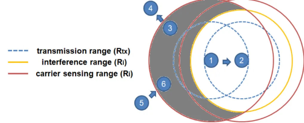
to the hidden node problem, exposed node problem and receiver blocking problem. For analyzing three problems, the carrier sensing range, the interference range and the transmission range are important. First, the following subsections explain the sensing area and then introduce the three problems.

2.5.1 Sensing area

The carrier sensing range Rcs is the range that the received signal power is larger than the carrier sensing threshold, that is, the minimum range allowed two concurrent transmitters. Otherwise, the node which received the signal is idle and the received signal is considered as noise. The Rcs depends on the carrier sensing threshold.

The interference range R_i is the range that the receiving node is inter- fered with an unrelated transmitter. The collision is occurred in the receiving node when a node withinRi of the receiving node transmits a packet. The R_i is the explained as

R_i=r·SIN R^γ¹ (2.3) wherer is the distance between the transmitter and the receiver, SIN R is the Signal to Interference plus Noise Ratio andγ is the path loss exponent.

The Table.2.3 shows the path loss exponent according to network environment [5]. In simulation, this thesis needs to set the value of the path loss exponent according to assumed network environment.

The transmission rangeTtx is the range that the transmitter transmits a packet successfully if the interference from other nodes is not occurred. The T_tx largely depends on the transmission power and the radio propagation properties (e.g., antenna gain).

2.5.2 Hidden node problem

The hidden node problem occurs that nodes can not hear each other. The Fig.2.4 shows the hidden node problem. Node 1 transmits a packet to node 2. Then node 3 can not hear that because node 1 is out of carrier sensing range of node3. The collision occurs when node 3 transmits a packet to node 2 during transmission of node 1.

The Fig.2.5 shows the hidden node range of node 1 and node 2. The hidden node area of each node is gray area in Fig.2.5. I denote by H^′(r)

(17)

Figure 2.4: Hidden node problem

Figure 2.5: The hidden node range

and r the hidden node area and the distance between node 1 and node 2, respectively. The H^′(r) can be expressed

H^′(r) =πR²_cs−2R²_cs [

arccos r

2Rcs − r 2Rcs

√

1−( r 2Rcs

)² ]

. (2.4)

2.5.3 Exposed node problem

The exposed node is in the range which is inside of Rcs of the transmitter and outside of Rcs of the receiver. The exposed node is the gray area in Fig.2.6. While node 1 transmits a packet to node 2, node 3 cannot transmit a packet to node 4 since node 3 hears the transmission of node 1 and defers own transmission. Also, While node 1 transmits a packet to node 2, node 5 cannot hear the response for the RTS/DATA since node 6 is blocked by the transmission of node 1.

(18)

Figure 2.6: The exposed node problem 2.5.4 Receiver blocking problem

The receiver blocking problem is occurred when a node cannot response for the RTS/DATA since the receiver is blocked by the transmission of other node. In Fig.2.7, node 1 transmits the RTS packet to node 2, node 3 is blocked because node 3 hears the RTS packet and waits for the NAV duration. Node 4 transmits the RTS packet to node 3, however, node 4 hear the response for the RTS packet since node 3 is blocked. Additionally, node 5 is blocked because node 4 transmits the RTS packet. The neighbors of a blocked node are unaware of the fact that the node is blocked, with result that the neighbor of a blocked node transmits a packet to a blocked node and cannot receive the response.

The blocked node need not be a hidden or an exposed node. For example, in Fig.2.7, node 3 can receive both the RTS packet and the CTS packet.

Thus, node 3 is neither a hidden nor exposed node and is blocked node.

(19)

Figure 2.7: The receiver blocking problem

(20)

Improving the throughput

and the fairness in single-hop

WLANs have become increasingly popular and widely deployed. Due to inherent simplicity and flexibility, DCF is preferred in the case of no base station such as vehicle to vehicle communications. Since all the nodes share a common wireless channel with limited bandwidth in WLANs, it is highly desirable that an eﬃcient and fair MAC protocol is employed. However, for the DCF, there is much room for improvement in terms of both eﬃciency and fairness. As demonstrated in [6], the fairness as well as throughput could significantly deteriorate when the number of nodes increases.

Although many researches have been conducted to improve throughput and fairness, few of them enhanced both of two performance metrics. In DCF, estimating the number of nodes is difficult because each node can reach or leave the network freely. For that reason, many researches have avoided estimating the number of nodes. In [7], although the number of nodes is estimated, however, it is complicated and it takes time to carry out this procedure. In [8] and [9], these schemes observe the average idle interval, and adjust the CW (Contention Window) in order to obtain a higher throughput. However these schemes do not estimate the number of nodes and have an issue in that the variation inCW of each node is large, which results in fairness degradation. In [10], based on [8], to improve the problem of fairness which is important for real time communication, authors introduced a method to achieve better fairness but this is still not enough. In this thesis, focusing on MAC protocol, I propose a novel protocol that each node estimates the number of nodes in a network with short convergence time and no overhead traffic burden added to the network through observing the channel, and nodes dynamically optimize their backoff process to achieve high throughput and satisfactory fairness.

The remainder of this chapter is organized as follows. In Section 3.1, I explain the background of this research. The Section 3.2 sorts out the

(21)

Figure 3.1: The monthly average mobile communication traﬃc in Japan problems in term of throughput and fairness. I introduce the related works that resolve these problems and improve throughput or fairness in Section 3.3. These related works are better than the conventional method in term of throughput or fairness, but not enough. In Section 3.4, I elaborate on our key idea and the theoretical analysis for improvement. Then I present in detail our proposed Optimizing Backoﬀ by dynamically Estimating Number of nodes OBEN scheme. Section 3.5 gives a performance evaluation and discusses the simulation results. Finally, concluding remarks are given in Section 3.6.

3.1 Background

WLANs have become increasingly popular and widely deployed. The Fig.

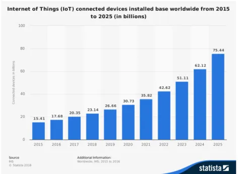
3.1 shows the monthly average mobile communication traffic (not include voice traffic) in Japan [11]. The monthly average mobile communication traffic increases year by year and is about 2000Gbps in 6/2017. It has increased 1.4 times in the last year. Also, the Fig. 3.2 shows the number of Internet of Things (IoT) connected devices worldwide from 2015 to 2025 [12]. For 2025, the IoT devices is forecast to grow to almost 75 billion worldwide. Since the traffic and the number of nodes are expected to increase, a correspoinding method is required.

WLANs have two channel access method, DCF and PCF, as shown in Ta-

(22)

Figure 3.2: IoT connected devices installed base worldwide from 2015 to 2025

ble 3.1. The access method PCF need the infrastructure but the throughput in high traffic and the fairness are high. By contrast, in DCF, the throughput in high traffic and the fairness is low since the infrastructure does not need. In view of future wireless communication traffic demands, the access method DCF that can configure the network flexibly becomes necessary. It is highly desirable that an efficient and fair DCF. Thus, this thesis focuses on DCF.

3.2 Problems of the conventional method

There are two problems in the conventional communication method DCF, therefore, the throughput and the fairness become low. In following, I give the problems of the conventional method.

• The throughput decreases when the number of nodes increases.

• The variation of theCW is large.

The node having packets for transmission senses the channel first. When the channel is idle for DIFS, the node carries out the backoff process. The node selects the backoff counter uniformly in the range [0, CW] and begins to decrease the backoff counter bye one for each idle time slot. The node can

(23)

Table 3.1: Access method in IEEE 802.11

transmit packets when the backoff counter is 0. In the case of collision, the node doubles itsCW until reaching a maximum valueCWmax, chooses a new backoff counter and starts the backoff process again. In the case of successful transmission, the node resets its CW to CW_min. Due to this algorithm, the throughput decreases when the number of nodes increases, as shown in Fig.3.3. There is the optimal CW that can maximize the throughput according to the number of nodes [13]. The node takes time until it changes from theCW_min to the around optimalCW and repeats many times. This problem is remarkable when the number of nodes increases.

In addition, The variation of the CW is large. The Fig.3.4 shows the variation of theCW. When the variation of theCW is large, a large diﬀer- ence occurs in the transmission between nodes. For this reason, the fairness decreases and the jitter is large. Therefore, the above problems need to be resolved.

3.3 Related works

Considerable research efforts have been expended on either theoretical analysis or throughput improvement ([6, 14, 15, 16, 17, 18, 19, 13, 20, 21, 22, 23, 24]). In [13], Cali et al. derived an optimalCW that can maximize the throughput. With the optimal CW, a backoff algorithm is proposed. Also, the method for estimating the number of nodes is proposed, however, this is complicated and it takes time to estimate the number of nodes, which is short of adaptivity to network changes. In [6], Bianchi used a Kim and Hou developed a model-based frame scheduling algorithm to improve the protocol capacity of the 802.11 [24]. In this scheme, each node sets its backoff timer in the same way as in the IEEE 802.11; however, when the backoff timer reaches zero, it waits for an additional amount of time before accessing the medium. Though this scheme improves the efficiency of medium access, the calculation of the additional time is complicated since the number of ac-

(24)

0.405 0.41 0.415 0.42 0.425 0.43 0.435 0.44 0.445 0.45

20 30 40 50 60 70 80

Throughput

Number of Nodes

Figure 3.3: Monotone functionf_idl(n) when the real value of n is 50 tive nodes must be accurately estimated. In [14, 15, 16], the works improve throughput and fairness for multi-rate traﬃc in the saturated case. How- ever, in [14], the MAC frame header contains the additional information, and the throughput becomes low in the non-saturated case. These works [15, 16] assume that the system environment is coordinated by an access point (AP). That is, they do not work without AP. In our previous study, a novel MAC protocol OSRAP was proposed [25], which can achieve a low packet delay and higher throughput. However, it needs to select a node as the head, which is not a perfect distributed protocol. In Idle Sense [8] and DOB [9], each node observes the average idle interval between two transmissions, and selects optimal CW according to the average idle interval to obtains high throughtput. However, the works cannot avoid the multiple transmissions from other nodes between two transmissions of a node and fairness is degraded. In AMOCW [10], based on Idle Sense, changes the method of collecting the average idle interval for preventing the multiple transmissions. With throughput like Idle Sense, AMOCW obtains fairness better than Idle Sense but not enough due to using AIMD (Additive Increase Multiplicative Decrease) algorithm. The fairness is another important issue in MAC protocol design [26].

Here, I propose a novel protocol OBEN to improve both throughput and fairness. OBEN estimates the number of active nodes in a simple but eﬀective way instead of the complicated method used before. Compared to the methods in [8, 9, 10], since each node in OBEN can correctly estimate the

(25)

0 100 200 300 400 500 600 700 800 900 1000 1100

0 2 4 6 8 10 12 14 16 18 20

CW [time slots]

simulation time [sec]

Figure 3.4: The variation of theCW

number of nodes and keep itsCW close to the same optimal value, OBEN can maintain fairness and keep the network operating with less fluctuation.

3.4 Analysis and the proposal of optimizing back- oﬀ by dynamically estimating the number of nodes

3.4.1 Motivation

In the IEEE 802.11 MAC, an appropriate CW is the key to providing throughput and fairness. A small CW results in a high collision probability, whereas a largeCW results in wasted idle time slots. In [13], Cali et al. showed that given the number of active nodes, there exists an optimal CW that leads to the theoretical throughput limit and when the number of active nodes changes, so does this optimal CW. Since in practice, the number of active nodes always changes, to let each node attain and keep using the corresponding optimal CW requires the estimation of the number of active nodes. However, previous methods for on line estimation and convergence time for all nodes are complicated since to estimate the exact number of nodes takes a long time. To get around this diﬃculty, this thesis is thus motivated to find another eﬀective method that leads us to the optimalCW and hence the maximal throughput.

(26)

I expect the improvement protocol to have several characteristics as follows

• no added overhead of measurement for understanding network situation.

• being concise and eﬀective.

• achieving both high throughput and comparatively good fairness.

One problem for DCF is that when traﬃc increases throughput will reach the upper bound and the maximum throughput is lower than PCF, so added overhead of measurement is not expected. In the situation where there is limited computation resource of a mobile node and a changing network, a concise and eﬀective protocol is desirable. For vehicle to vehicle communication, real time data needs to be sent with little delay and each vehicle needs a minimum data rate for urgent data transmission even in a saturation case, so both high throughput and comparatively good fairness are required. I try to get the necessary information for optimizing transmission in a wireless network by listening to the wireless channel, which is simple since the DCF is in fact built on the basis of physical and virtual carrier sensing mecha- nisms. As shown below, I obtain the necessary indexes to give an improved protocol through listening to the wireless channel.

multi-hop wireless networks are necessary for systems such as vehicle to vehicle communications. The DCF is preferred since it can work without AP. In multi-hop wireless networks, the throughput becomes low because of hidden terminal problems and a multi-channel is an eﬀective method in that a group of nodes communicates with a single frequency channel.

This chapter assumes that the nodes of network communicate with each other using a certain frequency channel in one hop area, while leaving the task of how to arrange frequency channel to each group as the next work.

The study about multi-hop wireless networks is described in chapter5. Here, I try to give an eﬀective protocol with high throughput and good fairness for one hop area.

In the following, I derive the relationship between the average idle interval and the throughput through analysis. Using the relationship, nodes can obtain the optimalCW and achieve the high throughput and the good fairness. For the purpose of simplicity, this thesis assumes the frame length is constant and give the simulation results with diﬀerent packet sizes.

3.4.2 Analytical Study

In the IEEE 802.11 MAC, an appropriate CW is the key to providing throughput and fairness. In [13], the DCF is analyzed based on the as- sumption that, in each time slot, each node contends for the medium with

(27)

the same probabilityp subject top= 1/(E[B] + 1), whereE[B] is the average backoﬀ timer and equals (E[CW]−1)/2. Since our OBEN would enable all the nodes to settle on a quasi-stableCW shortly after the network is put into operation, for simplicity this thesis assumes that all the nodes use the same and fixedCW. Consequently, I have

p= 2

CW + 1 (3.1)

as all the expectation signs E can be removed. Channel events can be thought of as three types of events, successful transmission, collision, and idle. Suppose every node is an active one, i.e., always having packets to transmit. For every packet transmission, the initial backoﬀ timer is uniformly selected from [0, CW]. For each virtual backoﬀ time slot, it may be idle, or busy due to a successful transmission, or busy due to collision. Ac- cordingly, I denote byP_idl, P_s, and P_col the probabilities of the three types of events, respectively. Thus, I can express the above probabilities as

P_idl = (1−p)ⁿ Ps = np(1−p)ⁿ⁻¹

Pcol = 1−Pidl−Ps (3.2)

where nis the number of active nodes. Thus, the throughput is expressed as

ρ= T P_S

t_sltP_idl+T_colP_col+T_txP_s (3.3) where T is the transmission time of one packet, t_slt is slot time, T_tx is the successful transmission duration andT_col is the collision duration. Our aim is to maximize throughput shown in equation (5.11). To this end, I need to obtain the optimal CW according to the network condition such as the number of nodes. In the following, I give the method for estimating the number of nodes on line by three parameters P_idl, Ps and P_col which can be obtained directly by listening to the channel for a certain interval.

Then, using obtained P_idl, P_s and P_col, I give the method for maximizing the throughput dynamically. Calculating the number of nodes directly by equation (3.2) is ineﬃcient and unrealistic. Here, I uses a simple and eﬀective method which is suitable for real time estimating. From equation (3.2), I have Pidl/ps = (1−p)/(np), then p = Ps/(nPidl+Ps). Substitute p in P_idl= (1−p)ⁿ, it becomes as following,

P_idl= (1− P_s nPidl+Ps

)ⁿ. (3.4)

Letf_idl(n) = (1−_nP_idl^P^s_+P_s)ⁿ, whereP_idl, Ps andP_col are known parameters and n is the unknown parameter that needs to be estimated. Then when

(28)

0 0.1 0.2 0.3 0.4 0.5 0.6 0.7 0.8

30 35 40 45 50 55 60 65 70 P_idl=0.605(p=0.01)

P_idl=0.077(p=0.05) f_idl(n) (p=0.01)

f_idl(n) (p=0.05) fidl(n)

Number of Nodes

Figure 3.5: Monotone functionf_idl(n) when the real value of n is 50 f_idl(n₀) =P_idl, n₀ is the needed value. I find that f_idl(n) is the monotone function. I take the derivative of f_idl with respect to n, and let _dn^df = [ln(1−_nP_idl^P^s_+P_s) +_nP^P^s

idl+Ps](1−_nP_idl^P^s_+P_s)ⁿ. It can be found that the second term is always plus. Letx = _nP^P^s

idl+Ps, then 0≤x≤1.Then, the first term of ^df_dn becomes ln(1−x) +x which changes from 0 to −∞when x changes from 0 to 1. So, it can be understood that ^df_dn is not plus.

I can estimate the number of nodes by the simple calculation method, without solving a complicated equation. As shown in Fig. 3.5, the monotone functionf_idl(n) always decreases as the number of nodes is increasing. Since P_idl is a known value, f_idl(n) should be adjusted in agreement with P_idl. When Pidl is equal to fidl(n), n is the number of nodes deployed in real network.

The above characteristic is favorable for estimating the number of nodes n which can be calculated by the following dichotomy. Supposing n is in a range [0, n_max], initially let n_try1 =n_max/2 and substitute it into f_idl(n).

Then comparef_idl(n_try1) withP_idl. If f_idl(n_try1)> P_idl, I should setn_try2 = [ntry1+nmax]/2. Otherwise, I should setntry2= [ntry1+0]/2 for the following calculation. Obviously, this method is simple and eﬀective. For example, whenn_max= 100, nodes just need to calculate four times to estimatenin the worst case with maximum error 3. In the following, I present the condition of high throughput. And then, I give the method of how to dynamically tune CW to enhance throughput and fairness. The average idle slot interval is denoted byLidl, it can be expressed as

L_idl = P_idl

1−P_idl. (3.5)

With equation (5.1), (3.2) and (5.14), this equation can be further written

(29)

as

L_idl = 1

(1 + 2/(CW −1))ⁿ−1

= 1

n_CW²₋₁+...+(ⁿ_i)(_CW²₋₁)ⁿ⁻ⁱ+...+(_CW²₋₁)ⁿ. (3.6) I can simplify the equation (3.6) as

Lidl= CW −1

2n . (3.7)

I can obtain the equation (3.7) when CW is large enough. As a matter of fact, this is the case when the network traﬃc load is heavy. In this case, to eﬀectively avoid collisions, the optimalCW is large enough for the approximation L_idl = (CW −1)/(2n) in our OBEN, which is also verified through simulations.

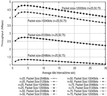
With Equation (5.11) and (3.7), thinking IEEE 802.11b, I can express the throughput as a function ofL_idl with SIFS=10s, DIFS=28s, ACK=304bits and time slot=9s, as shown in Fig. 4.1. From the figure, first, I find that every curve follows the same pattern; namely, as the average idle slot in- tervalL_idl increases, the throughput first rises quickly, and then decreases relatively slowly after reaching its peak. Second, although the optimal value of Lidl that maximizes throughput is different in cases of different frame lengths, it varies in a very small range, which hereafter is called the optimal range ofL_idl corresponding to different frame lengths. Finally, this optimal value is almost independent of the number of active nodes. Therefore,Lidl

is a suitable measure that indicates the network throughput. If nodes can estimate the number of nodes correctly, they can set the optimal CW by Lidl and nto achieve high throughput.

In Fig. 4.1, it can be observed thatL_idlis almost a linear function ofCW when CW is larger than a certain value. Specifically, in the optimal range of Lidl, say Lidl = [4,6]. From the above equation (3.7), according to the number of nodes, each node can set the optimalCW thatCW = 2nL_idl+ 1.

Since I am interested in tuning the network to obtain maximal throughput, given the linear relationship, I can achieve this goal by adjusting the size of CW. In other words, each node can estimate the number of nodes and adjust its backoﬀ window accordingly so that the throughput of the network is maximized.

3.4.3 OBEN Scheme

As mentioned above, I can obtain the optimal CW by Eq. (3.7) by using the estimated number of active nodes. Hence, each node can adjust itsCW dynamiclly and tune the network to deliver high throughput. To obtain the

(30)

1 1.5 2 2.5 3 3.5 4 4.5 5

0 5 10 15 20 25 30

Throughput (Mbps)

Average Idle Interval(time slot) Packet size=2048bits (n=25,50,75) Packet size=5120bits (n=25,50,75) Packet size=10240bits (n=25,50,75)

Packet size=12000bits (n=25,50,75)

n=25, Packet Size:2048bits n=25, Packet Size:5120bits n=25, Packet Size:10240bits n=25, Packet Size:12000bits n=50, Packet Size:2048bits n=50, Packet Size:5120bits

n=50, Packet Size:10240bits n=50, Packet Size:12000bits n=75, Packet Size:2048bits n=75, Packet Size:5120bits n=75, Packet Size:10240bits n=75, Packet Size:12000bits

Figure 3.6: Throughput with average idle slot interval

P_idl, PsandP_col, I can count the number of idle slots (C_idl), collisions (C_col) and successful transmissions (C_s) individually. To avoid occasional cases, C_idl, C_col and C_s are expected to be measured in resetting the counters before a transmission. TheP_idl, Ps and P_col can be calculated as

Pidl = C_idl C_idl+Cs+C_col Ps = Cs

C_idl+Cs+C_col P_col = Ccol

C_idl+C_s+C_col (3.8)

Since diﬀerent MAC protocols have diﬀerent definitions of time interval such as DIFS, SIFS, Cidl may need to be adjusted. A node calculates the CW before packet transmissions. After newCW (newCW) is obtained, the CW can be updated as

CW =β·CW + (1−β)·newCW (3.9) whereβis a smoothing factor with the range of [0,1]. Fig. 3.7 shows the sizes of CW of a node with simulation time when the β is changed. The higher β leads to stability but maybe reduces adaptivity to network changes such as traﬃc and active nodes. In OBEN, the sizes of CW are largely varied by little changes in the probabilities of idle, successful transmission and collision, which results in degraded throughput and fairness. For minimizing

(31)

200 400 600 800 1000 1200

0 20 40 60 80 100 120 140 Number of Nodes : 70

CW sizes of a node

Simulation Time (sec) OBEN (β=0.2) OBEN (β=0.5) OBEN (β=0.8)

Figure 3.7: CW sizes with simulation time when theβ is changed the variation of CW and adjusting the changes in the number of nodes, I setβ = 0.8 in simulation results in the next section. In the following, I give the tuning algorithm.

1. A node, say Node A, begins listening to a channel and counts events of idle slot, successful transmission and collision individually.

2. When Node A needs backoﬀ and the number of packet transmissions reaches a certain number, it calculates the optimal CW as a new CW and resetsCW according to Eq. (3.9).

3. It resets counting events of idle slot, successful transmission and collision.

The certain number of packet transmissions needs to be set appropri- ately. When the number is small,CW changes rapidly with network changes.

In contrast, if the number is large, the network can have higher stability but is short of adaptivity. In the following simulation, I set a certain number as 2. Ideally, each node should have the same CW when the network en- ters into a steady state in saturated case; in reality, each node sets itsCW around the optimal value. Using this method, high throughput and good fairness are achieved, which can be found in the following simulations.

3.5 Performance evaluations

In this section, I focus on evaluating the performance of our OBEN through simulations, which are carried out on OPNET Modeler [27]. OPNET Mod- eler, currently known as Riberbed Moder [28], is a commercial simulator that can be used for a fee. It can perform advanced protocol model de- velopment and flexible scenario creation. For comparison purposes, I also present the simulation results for the IEEE 802.11b DCF. In all the simu-

(32)

Table 3.2: Network configuration Parameter Value

M inCW 31 M axCW 1023

SIFS 10 µsec DIFS 50 µsec Slot time 20 µsec Bit rate 11 Mbps Table 3.3: Backoﬀ parameters

Parameter Value

Lidl 5

β 0.8

Maximum number of nodes 100

lations, I consider the MAC scheme, where RTS/CTS mechanism is used.

Generally, OBEN works for all IEEE 802.11 family. Though many improved IEEE 802.11 MAC protocols have been proposed, the evaluation condition and environment are diﬀerent. Here, I compare our proposed OBEN with AMOCW proposed in [10] which achieved the best results and Idle Sense [8]. In view of the fact that the performance of IEEE 802.11 standard is well known, in this section, I also use IEEE 802.11b as the standard reference.

The related parameters of IEEE 802.11b are shown in TABLE 5.1 and the OBEN-specific parameters in TABLE 3.3. The L_idl is 5 for obtaining high throughput as shown in Fig. 4.1.

I assume that network nodes are distributed at random in a round area with a 200 meter radius and that all nodes are in the communication range.

Without a specific application, I assume that each node generates traffic according to a Poisson process with the same arrival rate. Since I focus on throughput in the saturated case, the throughputs with different arrival distributions are slightly different in the border around the non-saturated and saturated case but the effects of an arrival distribution are extremely small. In the fully non-saturated case and saturated case, the throughputs are almost similar. Each node selects another node at random as a receiver.

The arrival rate is kept increasing until the network is saturated. As shown below, OBEN exhibits a better performance.

3.5.1 Throughput

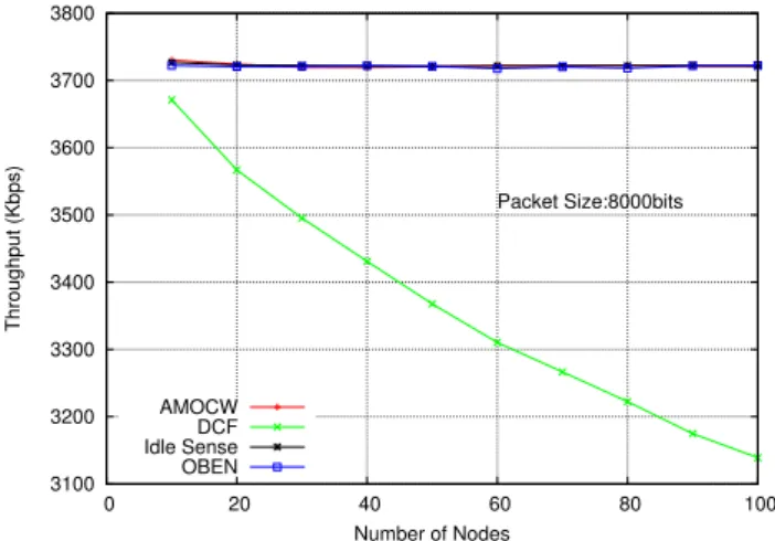
Firstly, I give the throughput of four schemes, i.e., OBEN, AMOCW, Idle Sense and DCF of IEEE 802.11b under different offered loads and pack- etsizes. Fig. 3.8 shows the throughput results with a different number of

(33)

3100 3200 3300 3400 3500 3600 3700 3800

0 20 40 60 80 100

Throughput (Kbps)

Number of Nodes

Packet Size:8000bits

AMOCW DCF Idle Sense OBEN

Figure 3.8: Throughput with node numbers Table 3.4: Throughput (Kbps) with node numbers

N AMOCW DCF Idle Sense OBEN

10 3730 3671 3727 3722

20 3724 3567 3723 3721

30 3720 3495 3723 3721

40 3719 3431 3721 3722

50 3721 3368 3721 3721

60 3722 3310 3722 3718

70 3721 3266 3722 3720

80 3723 3222 3722 3718

90 3721 3175 3722 3722

100 3722 3139 3721 3723

nodes. The packet size is the size of payload data at MAC layer and does not include MAC overhead, which is one reason that the simulation results are lower than the theoretical values. The throughput is the total data traﬃc successfully received.

The throughput of IEEE 802.11 DCF decreases with the number of nodes increasing. When the number of nodes changes from 10 to 100, the throughput of IEEE 802.11 DCF falls from 3.68Mbps to 3.12Mbps, about 18% down.

On the contrary, our proposal OBEN, Idle Sense and AMOCW have almost no changes. The throughput of OBEN is almost same as that of Idle Sense and AMOCW, that the three lines of OBEN, Idle Sense and AMOCW over- lap each other in the figure. The detail can be found in the Table 3.4 with throughput data. While achieving as high throughput as AMOCW, OBEN has a better fairness, which will be shown in the next section.

(34)

3.5.2 Variation of CW and Fairness

Many researches deal with the fairness of networks. For different applica- tions, there are different requests. Here, I omit the detail and just evaluate this item in way of an intuitive awareness. IEEE 802.11 applies an exponen- tiation backoff algorithm which can disperse retransmission timing among collision nodes. However, some nodes may defer time too long so that they cannot transmit for a long interval, which results in poor fairness as occurred in AMOCW and Idle Sense. I can evaluate the fairness of OBEN with AMOCW through the observation ofCW variation in the saturation case. Fig. 3.9 shows the instantaneous value ofCW of a node in simulation.

At the beginning, 20 active nodes compete for the channel. After 50 seconds, 40 nodes start competing for the channel. Then, the 40 nodes leave after 100 seconds. From Fig. 3.9, OBEN is coincided with the analysis results and has good scalability in runtime. In contrast, CWs of AMOCW, Idle Sense and DCF vary intensely when the number of nodes increases quickly, which means a big change of the transmission interval in view of the time dimension and this results in poor fairness and high jitter. Fig. 3.10 shows the instantaneous value of CW and the retransmission attempts of a node.

OBEN has a small variation of CW and the number of retransmission at- temps because OBEN always obtains CW around the optimal value. In contrast, in AMOCW, the variation of CW is large, which causes many retransmission attempts and decreases fairness as described below.

To evaluate the fairness of OBEN, I adopt the following Fairness Index (FI) [29] that is commonly accepted:

F I = (∑

i=1Ti/ϕi)² n∑

i=1(T_i/ϕ_i)² (3.10)

where T_i is throughput of flow i, ϕ_i is the weight of flow i (normalized throughput requested by each node). Here, I assume all nodes have the same weight in simulation. According to equation (4.7), F I ≤1, where the equation holds only when allT_i/ϕ_i are equal. Normally, a higher FI means a better fairness.

Figure 5.9 shows the results with a diﬀerent number of nodes from 10 to 100, in which the results of OBEN, AMOCW, Idle Sense and IEEE 802.11 DCF are put together for comparison. From the figure, I can see that our proposal OBEN has the best fairness among the four protocols. In particular, when the number of nodes increases, the fairness of OBEN has no obvious changes. On the other hand, Idle Sense degrades fairness heavily and becomes lower than DCF from 50 nodes, which results from each node of Idle Sense not knowing the correct CW to which it should set and it just increases or decreasesCW according to the common channel situation indicated by the average idle interval. Thus, a lack of balance occurs among nodes in the network. The same tendency also can be found for AMOCW

(35)

0 200 400 600 800 1000 1200 1400

0 20 40 60 80 100 120 140

CW sizes of a node

Simulation Time (sec) (20 -> 60 -> 20 nodes) AMOCW

DCF Idle Sense OBEN OBEN Analysis

Figure 3.9: CW sizes of a node with simulation time

except that the fairness is improved. For Idle Sense and AMOCW, the fairness changes periodically, which is thought to be the result of AIMD algorithm used in Idle Sense and AMOCW. From the figure, I can see that the fairness of OBEN is dramatically enhanced.

3.6 Conclusions

In OBEN, nodes just need to confirm if the media is busy or idle to obtain the number of idle slots, successful transmissions and collisions through listening to a wireless channel without added overhead. And then using a simple and eﬀective method, OBEN estimates the number of nodes to set an optimal CW. Meanwhile, though all the nodes may not have the same CW, occasionally, each node can adjust its CW rapidly and keeps close to the optimal value, which means they will fairly share the common wireless channel. This leads to good fairness.

Through both analysis and simulation, our scheme has the following advantages. First, the method of estimating the number of active nodes of a channel is simple and effective for each node to grasp the network traffic situation. In addition, the average idle length is insensitive to the change in packet length or the number of active nodes. Each node can adjust its backoff process simply, avoiding complex calculations. Second, compared with the Idle Sense and AMOCW, OBEN achieves better fairness with almost the same throughput.

(36)

0 200 400 600 800 1000 1200 1400

0 20 40 60 80 100 120 140 0

5 10 15 20 25 30

CW sizes of a node Retransmission Attempts of a node (packets)

Simulation Time (sec) (20 -> 60 -> 20 nodes) AMOCW CW OBEN CW AMOCW Retransmission OBEN Retransmission

Figure 3.10: CW sizes and retransmission attempts of a node with simulation time

0.8 0.82 0.84 0.86 0.88 0.9 0.92 0.94 0.96 0.98 1

0 20 40 60 80 100

Fairness Index

Number of Nodes AMOCW

DCF Idle Sense OBEN

Figure 3.11: Fairness Index

(37)

(38)

Improving the throughput

and the fairness in single-hop with QoS

The Chapter 3 proposed the new MAC protocol OBEN. Whereas, OBEN does not take QoS into account. The real time traffic need to be provided with the required throughput and delay guarantees. According to the kind of traffic, the node must control the transmission opportunity. Thus, this chapter proposes a novel MAC protocol scheme that Optimizing Backoff with better QoS, named as OBQ. OBQ, based on OBEN, can improve the throughput and the fairness with good QoS.

The remainder of this chapter is organized as follows. The Section 4.1 describes the problems of the conventional method. I introduce the related work in Section 4.2 I elaborate on our key idea and the theoretical analysis for improvement in Section 4.3. Then I present our proposed scheme OBQ in detail. Section 4.4 gives performance evaluation and the discussions on the simulation results. Finally, concluding remarks are given in Section 4.5.