払
鶉1冊
文
On the Numerical Analysis of Elliptic Partial Differential Equations by Successive Overrelaxation Method.
Jiro SHIMoNlsHI*
Nobuaki ToMiTA* Hiroshi NIKi** Hideo
(Received September 30, 1972)
SAWAM1**
We have proposed formerly the method of using S.O.R. in which successive better estimate of the apploximated accelerating factor are obtained by using the property with residuals, during the couse of solution.1),2),3) in this paper, we propose the new technic 6f obtaining the estimate of optimum accelerating factor by using the property with residuals. By applying our method, we solve the Laplace/s equations with Dirichlet boundary condition and with the mixed boundary condition in 2−dimensional coordinate, and in axlally−Jsymmetric regions, and compare its effectiveness with that of other method.
Introduetiom :
The successive over−relaxation method(hereafter referrd to as S. O. R.) is known an effective iterative method for sohTing the difference analogue of an elliptic partial differ−
ential equation. lt is found that the numerical solution of ellipt・ ic partiai differential equations is obtained by solving linear algebratic equations which can be expressed in the form:
五κ緬, (1)
where, matrix A is symmetric matrix and x, b are colum vector, By resolving matrix A into 1−L−U and applying S.O.R., formula (1) is expressed as forrnula (2).
(1一 toL) x( le)= {o) E7 一(to−1) 1} x(ie 1)十 ob, (2)
where o is a parameter known as accelerating factor and the rate of conYergence of iterative皿ethod depen ds strong−
ly on this accelerating factor. And x(k), x(leTl) are values which are obtaine d bothle th time−step and (k−1) th time−step.
Iis unit matrix and L, U are lower and upper triangu!ar matrices with null diagonals. The convergence of formula
(2) is governedby the lqrgest o± the absolute values of the eigenvalues of the matrix M, as shown formula (3) :
!1f一 (1一 tuL)一1 {toU一(to一1) 1} (3)
By YQng!s4)theory and others the optimu皿aecelerating factor toopt which produces the best rate of convegence is given by the following:
The relationship among the eigenvaluesλ,i ofノ賦 acceレ eratig factorω, and the eigenvalues of matrix(L十U)is given by the following ;
Jei.2一(Ni十to−1)2/to2Ni. (4)
From formula (4), re,pt must satisfy the following relation of formula (5):
Q)oPt21bmax2_4(ωoPt一一一1);0,
コ に コ ロ ら ロ ロ サ ヒ ロ ロ カ タ
て ド コ
an(1 trom mls relauon lt ls possloleτo qelmeωoρ≠:
ω。毎一2/(1+[/. 1一砺僻2,
where鯨ακis Lhe maximum ofμか
If we define the displacemen£vector atんth time−step byformula(7):
θ(々)=X(彦+1)一X(々)
,
the norm of arbitrary displacement vector sat童sfies
li斑 IIθ(々+1) li/ ll 訊々) i{ = λmax.
々→。。
A鶏dthen, we define
λた剰e(k+1)1/11d釧.
*DePa吻ten彦。/Elec〃ical Engineering
Tsayama Technical College**DePartment of APplied Mathematics
Fασ%〃ッ。/ScienceOfeayama. Co〃ege o/Science
(5)
(6)
(7)
(8)
(9)
Since we can consider that Xle continually increases, the assirmed limit value Nmax can be estimated from the rela−
tion between le and Xk.
Kulsrud, Carr6 and others have publised the method of esti一
一27マー
津山高専紀要 第3巻 第3号(1973)
mate Xmax during the course of solution, and then estima−
ting of apploximated toopt by using for皿ula(8),(9).
Kulsrud s method is following procedure :
(1) The first five iterations are performed by using with 1.5 value.
(2) Assumed X... is obtained from formula (9). Find pmax from eqttation (4) and then, an improved estimate of di is oPtained from formuls (6) . (3) This process is repeated until the new estimate on to amounts to the last estimate which is desired beforehand.
This final value of tob is used for remainder of the calculation. Successive estimate of tu is each used for five iterations.
The precedure of Carre s method is fol!owing:
(1) The first iteration is performed by using to with unity value. The next twelve iterations are performed by using with 1.375 value. Successive esti皿ate ofωis each used for twelve iterations,
until a fimal estimate ot ob has been made.
(2) Next, in order to estimate Xmax at the end of the group of twelve iterations, the values of II e/le)[1 are for皿ed during the last four of these. From the values of I l e(le)Il, three successive values of p(k)
are obtained by formula (10) :
ρ(k−2)1=:Ue(le−2)1/」e(le−3)ll, P(k−1)=ldん一1)1凶2(le−2)1
P(k)一ile(le)II/1[e(k i)ll. (10)
(3) By using Aitken−extrapolation, )... is estimated shown as formula (11).
X...#P(h−2)一{P(leml)一p(k−2)}2/{p(le−2)十p(fe)一2p(fe−1)},
(11)
and ILmax is found from equat ion (4) , and then an improved estimate of to is obtained from formula
(6).
(4) An estimate to is deemed satisfactory if arithmetic difference Ato between this estimate and the previos one satisfies the condition:
dto/(2−to)ZO.05, (12)
and if condition has been satisfied, o is deter−
rnined as final estimate valne of tob.
(5) This final tob is used for the remainder of calcu−
Iations.
There seem to be inherent dangers the use of above
mentioned technique. That is;un!ess the value of pti
obtained by these method is equal to tu 一1, the process will cQntinually increaEe cob which tend to a),pt in formula(6). lt indicats that the process should a1ways started with an initial tu less than the suspected tob. When an tub larger than tu,pt is predicated by the process, ob will no lon一 ger be able to converge to tuopt. Accordingly, it is important how to select an initial to. And it is necessary not to per−
mit too large an overestimate of tob. But this can be con:
trolled by the termination procedure for the tob process.
That is;as above皿entioned, they have predicated otopt
when arit.hmetic difference between improved ob and pre−vious one beco皿es less than a small amount.
Outline of the kulsrud/s and Carr6 s method was dis−
dcrive above. ln thi$ explanation, in order to estimate tuopt, Kulsrud has selected that initial tu is 1.5 value, and Carre has selected 1 value. And, they have applied only some kind probiem and have published.
Therefore we attempted solving the problem in axially symmetric co−ordinate by using their method. From these results, we have found that their method could not continue the S.O. R., because tob falled into complex values during the caluculation for some size models. When its condition had been yielded, they have never explained as to just ofter procedure in their reports.
By introducing the new idea how to estimate Xmax and
determine the oept. We attempted the new method which
can be able to use for both the problem on 2−dirnensional Cartesian co−ordinats and axially symmetric co−ordinats.Theory :
We also attempted to estimate Xma. by using the ratios of successive norm of displacement vector.
That is, ptmax is estimated by using the ratios of succes−
sive I〕or皿of displacement vector shown as formula(13):
Xmax.t{P(k)十P(fe−i)十P(km2)]/3,
(13)
where カ@一2)= 1]e(k−2)1「/11e(た一3)ll,ρ@一1)=11θ⑭一1)」/idle一2)1,
P(fe)一le(le)ll/][e(le−i):.
The norm ll e㈲[i used for estimateλ,max is the arithmetic sum of the absolute length of the displacement vector朕々).
That is,
れ
ie(た)1=ΣコIXi(k)一Xi(彦一1)i.
ゴ=1
By usingλ,max eStimated from the abQve. pro66ss,βmbx.is
一 278 一
S.0.R.法を用いた楕円型偏微分方程式の一解法 下西・富田・仁木・沢見
assumed from equation (4) and to is estimated from formu一
}a (6). By applying our method, we have estimated to by every nine iteration.
In order to predicat toopt, it was important how to con−
troll the procedure the tob process. We have empirically found:/ the following :
An improved to is obtained after some number of iteyations,
and when to is less than toopt, the norm, just after o has been7improved, is larger than the norm just before w had
∈轄胤「...tUt.h.へ
beeltt imptoved. But as to comes near o,pt, the above men−
tioned relation is reversed. And we have proposed formaly the method which predicat di,pt by using the property with residuals, as following;
we have empirically noticed that, after the optimum value, all eil」一 are positi v−e, w neR Lhe factor is larger than the optimum value, howerer, some eis are found to be negative. (reffer to 1), 2) )
In this paper, by applying this property, we have de−
termined the final estimate value of ob Our method is summarrized as follows:
(1) The first iterat ioR is performed by using e) which is given by X...==cos Cva/(N)1/2)
for spuare region. Where, N is mesh to be calcu−
lated.
(2) And then, by using the ratios of norm p(le−2), p(h−1),
p(k), Xmax 1s estimated from formula(13) .
(3) pmax is assumed from equation (4) and the estimate of to is obtained from formula (6), where, in the equation (4) , the previous to is used.
(4) Successive estimate of to is each used by every nine iterations and this process is repeated until the norm,
just after to has been improved, is smqller thap the norm just before lo had been improved and if nega−
tive sign of residuals ei appears ten per cent of the mesh to be calculated, its tob is considered overesti−
mate, then, this tub is multiplied by O.985 value.
Then, the then to is assumed the final value of tob (5) Remainder calculatiofl is performed by using this final tub We have empirically determined 9 value which will be necessary iteration number in order to estimate better tob and O . 985 value which is a mul−
tiplier when cab is judged overstimate by our method.
estimated by using other method for Dirichlet problem of rectangular region in 2−dimensional Cartesian co−ordinats.
It was found from this resu!t, that our method produced better optimum accelerating factor than the others.
Ta湿e 1
Comparison of to opt estimated by our method with by others.size
一.
Carre s
method
20 × 15 1.5660
25 × ・9..O
30 ×. 25
1.6806 1.7498
1 Kulsrud s i
method
Our
me・ thod1.7112
1.68e51.7783 1.7465
1.8エ94:一
1.7589
40×30 1.8569 1.7992
a)oPt
1.6725 1.7413 1.7859
1.8259・
Table 2 gives a comparison cti TLhe nurriber of i i eratives when tuopt is obtained various method, where, the problem is the solution oi Laplace s equation for axja].ly−synimetric
Ta魏e 2
Comparison of our rnetlaod and other method for axially symmetric region.size
Experimental results;
Carre s
method ﹇
Kulsrud s
method
25 × 20
N ×
e)f
×
Our method
35 × 20
109
1.883e
N ×
×
wf
13 × 13
N .一
tuf
×
52
r
1.7685
78
:
1.8202
15 × 15
17 x 17
N
tof
N
tof
20 ) 20
25 × 25
30 × 30
Table 1 gives a comparison of toopt which have been estimated by using our method with toopt which have been
40 × 40
N
ωノ
N
tof
N
ωノ
N
wf
41
ト
E 1.6754
× × 1
42
.一
×
×
×
×
×
85
1.8709
×
no
convergence
×
×
1.7038 67
1.7933 81
1.8394 99
1.8454 118
1.8621 125
1.8839
N : lteration number for convergencetof : Final value of acceleratihg factor
一 279 一
津山高専紀要第3巻第3号(1973)
region. We could not obtain a solution for X in Table 2,
because the accelerating factor had cornplex value . lt is apparent from above results, that Kulsrud s and Carre s method could not obtain the solution for the models like these.
Our皿ethod was slso tried on a region with rectangular
Dirichlet boundaries coverd and mixed boundaries condi−
tion which two of the boundaries had Neuman conditions
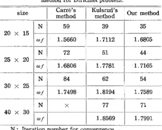
applied.Table 3
Comparison of our method and other method for Dirichlet problem.In each cace. a maximum residue less than 10−5 time
the largest boundary value was required to terminate the solution.
Conculusion:
size
20 × 15
25 × 20
30 × 25
4e × 30
N
of
N
tof
N
tuf
N
dif
Carre s 皿etho(1
59
1.5660 72
1.6806 84
1.7498
×
Kulsrud s
method
39
1.7112 51
1.7781
62
1.8194 77
1.8569
Our method 35
1.6805
44・
・1.7165
54
1.7589
In some models which we attempted, it was found that Kulsred s xnethod was mo.re effective than Carre s one, but as for special models, Carre s was more effective than Kulsrud s. But it is considered that both their method can not to use for some kind of problem.
On the other hand, our method can using these problem and it is clear that our method requier fewer iterations than the others. Especially, for a problem with mixed boundary condition, as is evident from above results our method is the most effective of all others.
In the field of engineering and the like, since Dirichlet problem is not used so much as mixed boundary condition proble皿, we consider that our method is more effective for mixed boundary condition in these fields. We hope to report in near future.
71
1.7991 N : lteration number for convergencetof: Final value accelerating factor
Table 4
Comparison of our method and othermethod for mixed boundary problem.
Acknowledgments: We used a HITAC−8400/65 in Data procssing Centre of Okayama College of Science, And NEAC−3200/30 in Tsuyama Technical College.
size
20 x 15
IN
25 × 20
30 × 25
40 .× 30
ωア
N
ωア
N
tuf
N
tof
Carre s
method Kulsrud smethod
107 81
1.7787 98
1.8848
×
199
1.8870
1.8766 113
1.9110 143 1.9309
184
1.9987
Our method 73
1.829695
1.8659114
1.8923143
1.9118 N : lteration number for convergencetof: Final value accelerating factor
References
(1) NIKI, H.: Practical technique for the successive over−
relaxation method , Electron. Lett., 1971,7, pp.173−174.
(2) RADLEY, D. E., DIRMIKIS, D., anq BIRTLES, A..B.:
Coment on practoal technique for the successi e over−
relaxation method, Electron. Lett., 1971, 7, p.369.
(3) NIKI, H., and others, : Relaxtion method for mixed boundary conditions ., Electron. Lett., 1971, 7, p.525.
(4) Young, D. M.: lterative method for solving differ−
ential equations of el]iptic type. , Trans. Amer. Math.
Soc., 1954, 76, pp.92−111.
(5) Carre, B. A.: The determination of the optimum accelerating factor for successive over−relaxation .,
Comput. J. 4, p.73.
(6) KULSRUD,H.E.: Apractical echnique for the deter−
mination of the optimum relaxation factor of the succes−
siveover−relaxation method ., Comm. Assoc. comp., 1961,
4, pp.184−187.
Table 3,4 give the itg. ration number up to convergence and final aceelerating factor and compare theml with others.
It is consider from these results that Carre s method is
insecure for the some models, because tob had cpmplex
value.一 280 一