Theoretical analysis of spin current induced in cold atoms with artificial

(1)

Theoretical analysis of spin current induced in cold atoms with artificial

spin-orbit coupling

人工スピン軌道相互作用を持つ冷却原子系で誘起されるスピン流に対する理論的解析

Department of Physics,

Graduate School of Science and Engineering, Tokyo Metropolitan University

Ryohei Sakamoto

2019

(2)

Abstract

Atomtronics, a technique to control atoms for an application of devices, has been studied in recent years. The purpose of this thesis is to propose a novel method to control atoms for the application to the atomtronics. To achieve this purpose, we use a spin current in a spin-orbit (SO) coupled cold atoms. The spin current, that is a counterflow of particles with diﬀerent spins, has attracted attention as a method to control electrons. On the other hand, the artificial SO coupled cold atoms were experimentally realized in 2011 and have been studied theoretically and experimentally. We can expect that a spin current can be formed in the SO coupled cold atoms because the SO coupling is known to induce a spin current and controlled because the cold atoms have various experimentally controllable parameters. However, little has been studied so far on the spin current in the cold atom. Therefore, we studied novel controllability of the spin current in the SO coupled cold atom.

An SO coupled Bose-Einstein condensate (BEC) was experimentally realized in 2011 and then an SO coupled degenerate fermions became available in 2012. In these systems, since the SO coupling was engineered in a neutral atom by dressing two atomic spin states with a pair of Raman lasers and an external magnetic field, it is called artificial SO coupling. In addition, some parameters such as intensity of the SO coupling can be experimentally tuned by the lasers and the external magnetic field in the artificial SO coupled cold atoms. Therefore, by investigating parameter dependence of the spin currents, we reveal controllability of the atoms in the artificial SO coupled Bose and Fermi systems. As a result, in the SO coupled Bose system, the spin current changes discontinuously and non-smoothly across the phase boundaries, while in the SO coupled Fermi system, the spin current changes continuously and smoothly at zero temperature.

On the other hand, Bose-Fermi mixture was experimentally realized and have been studied from diﬀerent viewpoints. Therefore, we can expect to realize an artificial SO coupled Bose-Fermi mixture in near future. In this system, since atoms of diﬀerent quantum statistics coexist under an influence of the SO coupling, novel phenomena can be expected. Based on these ideas, we investigate a ground state and a spin current in a mixture of fermions and SO coupled bosons. The ground states are calculated in the SO coupled Bose-Fermi mixture with high density or low density of the atoms by using a variational method and some approximations such as tight-binding approximation. For the high density, the fermions have a large influence on the Bose system, while, for the low density, the fermions have little influence although the relative amounts of the bosons and the fermions are comparable in the two cases. In addition, we show that the spin current of the

(3)

fermions changes discontinuously and non-smoothly across the phase boundaries of the bosons.

(4)

Introduction

Atoms trapped and cooled in ultra-low temperature is called cold atom. Cold atom can be experimentally realized and exhibit a variety of quantum phenomena. One of useful features of the cold atoms is controllability of physical parameters including interaction strength between the atoms[1, 2]. Taking advantage of the features, we can create various interesting atom systems. Particularly, in 2011, a spin-orbit (SO) coupled Bose-Einstein condensate (BEC) was experimentally realized[3] and then an SO coupled degenerate fermions became available[4, 5]. In these experiments, SO coupling was engineered in a neutral atom by dressing two atomic spin states with a pair of lasers and it is called artificial SO coupling. To explore rich properties of SO coupled BECs and degenerate Fermi gases, the SO coupled cold atoms have been studied theoretically and experimentally[6, 7, 8, 9, 10, 11, 12, 13, 14, 15, 16, 17, 18, 19, 20, 21, 22, 23, 24, 25, 26, 27]. In addition, another effort was made for simultaneous cooling of bosonic and fermionic atoms[28, 29]. The mixture systems where atoms of different quantum statistics coexist could have a variety of aspects and have been studied from different viewpoints[30, 31, 32, 33, 34].

On the other hand, atomtronics, the study of atomic transport phenomena for the application to devices, has attracted attention[35, 36, 37, 38]. In the atomtronics, a realization of a novel device unlike electronics can be expected because electrons, that is used in electronics, are Fermi particles with charge whereas atoms, that is used in atomtronics, are neutral Fermi or Bose particles. In our study, to propose a novel method to control atoms, we focus on a spin current. Spin current is generally defined as a counterflow of particles with diﬀerent spins and various methods to induce and control a spin current, that is called spintronics, have been proposed[39, 40, 41, 42, 43, 44, 45, 46, 47, 48, 49, 50]. Since it is known that spin current is induced by SO coupling, we can expect that atoms can be controlled by spin current in the SO coupled cold atoms.

In this thesis, we investigate the ground state and the spin current in the three types of artificial SO coupled cold atoms. The original results are to show the ground state phase diagram in the SO coupled Bose-Fermi mixture and the controllability

(7)

of the spin current in the SO coupled cold atoms. In the following chapters, we first derive the definition of a spin current and review the experimental method to realize the artificial SO coupled cold atom. Afterwards, we show the ground states and spin currents in the artificial SO coupled Bose system, the artificial SO coupled Fermi system, and the artificial SO coupled Bose-Fermi mixture, respectively. The details are shown in the followings.

As a ready to analyze a spin current, in Chap. 2, we show the properties of particle and spin currents in the system with an arbitrary magnetic field and SO coupling. To define particle and spin currents, we first derive the conservation laws of particle and spin from U(1) and SU(2) symmetry. Next, we consider the eﬀect of a magnetic field and SO coupling on the currents. In the latter half, the relation between the currents and an unitary transformation and the condition to induce currents are shown.

In order to experimentally create SO coupling in a cold atom, it is necessary to tune parameters in the cold atom with artificial gauge field[51]. Therefore, in Chap.

3, we review the experimental method to realize the cold atoms with artificial gauge field and artificial SO coupling, respectively. In addition, we show that the intensities of the SO coupling and eﬀective magnetic field can be controlled by the external lasers and magnetic field in the artificial SO coupled cold atoms.

Based on the above chapters, in Chaps. 4, we discuss an artificial SO coupled Bose system. As a first step, we analyze a non-interacting Bose system where all the bosons behave as a single-particle. The ground state of the interacting Bose system have been investigated in the previous studies by using a variational method[8, 9, 10, 11, 15]. Therefore, we review the method to obtain the ground state phase diagram and show the ground state phase diagram and the spin current of the bosons.

In the next chapter, we show the ground state and the spin current in the artificial SO coupled Fermi system without the interaction. As a result, we can see that the ground state is classified by the diﬀerence of Fermi sphere and that the spin current of the fermions has a characteristic property unlike that of the bosons. In addition, we investigate the eﬀect of the weak interaction on the Fermi system and show that it is negligible.

In Chap. 6, we consider the mixture of fermions and SO coupled bosons and show the ground state phase diagram and the spin current of the fermions. Since the SO coupled Bose-Fermi mixture is a novel system that had not been studied, all results in this chapter are original. We analyze the ground states of the bosons in the Bose-Fermi mixture without and with Bose-Fermi spin interaction by using the variational method same as in Chap. 4 and some approximations. In addition, the spin current of the fermions can be calculated in the same way as in Chap. 5 in the Bose-Fermi mixture with Bose-Fermi spin interaction. Finally, in Chap. 7, we conclude above results.

(8)

Chapter 2

Spin current

Spin current is a counterflow of particles with diﬀerent spins. Recently, spintronics, the study of spin-dependent electron transport phenomena in solid-state materials, has attracted attention[39, 40, 41, 42, 43] and various methods to induce and control a spin current have been proposed[44, 45, 46, 47, 48, 49, 50].

In this chapter, as a ready for the following chapters, we discuss the properties of currents induced in the system of spin-1/2 particles with a magnetic field (Zeeman eﬀect) and spin-orbit (SO) coupling. By using the invariance of Lagrangian, in Sec.

2.1, we derive the conservation law of particle and show the eﬀect of a magnetic field and SO coupling on the conservation law. In the next section, we derive the (non- )conservation law of spin in the same way and define the spin current. Since the definitions of the particle and spin currents are changed by a unitary transformation of the wave function, we show the relation between the currents and the unitary transformation in Sec. 2.3. Finally, in Sec. 2.4, we analyze the properties of particle and spin currents and show the conditions that the currents are induced.

2.1 Conservation law of particle and particle current

Let us consider the system of spin-1/2 particles with a magnetic field (Zeeman eﬀect) and SO coupling. The Lagrangian is given by

L = L0+LB+Lso, (2.1)

L0 =

∫ dr

{

ψ^†(r, t) [

i¯h∂

∂t− ¯h²∇² 2m +µ

]

ψ(r, t) }

, (2.2)

L_B =

∫ dr{

ψ^†(r, t) [B(r)·σ]ψ(r, t)}

, (2.3)

L_so =

∫ dr{

ψ^†(r, t) [B_so·σ]ψ(r, t)}

, (2.4)

where ψ(r, t) is the field operator, m is the mass of particles，σ = (σ_x, σ_y, σ_z) is 2×2 Pauli matrix, and ∇ indicates the gradient with respect to r. In Eqs. (2.3)

(9)

and (2.4), B(r) is an arbitrary magnetic field and B_so = (B_so,x, B_so,y, B_so,z), where B_so,j =a_j ·(−i¯h∇) and a_j = (a_xj, a_yj, a_zj) is an arbitrary vector corresponding to a strength of SO coupling ¹⁾. In the following, we will derive the conservation law of particle from the rotational symmetry in the phase factor of the wave function of the system[43, 49].

2.1.1 Conservation law of particle

Firstly, we analyze the system without the magnetic field and SO coupling described by Eq. (2.2). Using scalar quantity φ(r, t) that is dependent on space-time, we consider the phase transformation of field operator

ψ(r, t)→e^iφ(r,t)ψ(r, t), ψ^†(r, t)→ψ^†(r, t)e⁻^iφ(r,t). (2.5) By substituting this field operator into Eq. (2.2), the Lagrangian is converted into

L₀ →L₀+

∫ dr

{ ψ^†

[

−¯h∂φ

∂t ]

ψ + i¯h²

2m

([(∇ψ^†)

ψ−ψ^†(∇ψ)]

·(∇φ) +ψ^†ψ(∇φ)² )}

. (2.6) When the phase φ is diﬀerentiable and a single-valued function of space-time, the original Lagrangian and the converted Lagrangian must describe the same physical phenomenon. Therefore, the first-order term of φin Eq. (2.6) must be zero. This means that the variation of the action δS₀ = δ∫_∞

−∞dtL₀ satisfies the following equation:

δS₀ =

∫ _∞

−∞

dt

∫ dr

{

−¯hψ^† [∂φ

∂t ]

ψ+ i¯h² 2m

([(∇ψ^†)

ψ−ψ^†(∇ψ)]

·(∇φ) )}

= ¯h

∫ _∞

−∞

dt

∫ dr

{[∂( ψ^†ψ)

∂t − ∇ · i¯h 2m

[(∇ψ^†)

ψ−ψ^†(∇ψ)]] φ

}

= ¯h

∫ _∞

−∞

dt

∫ dr

{[∂ρ

∂t +∇ ·j ]

φ }

= 0. (2.7)

From this equation, we can obtain the conservation law of particle

∂ρ

∂t +∇ ·j = 0, (2.8)

1)The SO coupling term in Eq. (2.4) can be written as

Bso·σ=(

px py pz

)

axx axy axz

ayx ayy ayz

azx azy azz







σx

σy

σz



, wherep=−i¯h∇.

(10)

where

ρ=ψ^†ψ and j =− i¯h 2m

[(∇ψ^†)

ψ−ψ^†(∇ψ)]

(2.9) are the number density of particle and the particle current density, respectively.

2.1.2 Particle current in the system with a magnetic field and SO cou- pling

Calculating the variation of the actions obtained from Eqs. (2.3) and (2.4) under the phase transformation (2.5), we analyze the eﬀect of the magnetic field and SO coupling on the conservation law of particle (2.8).

Firstly, since the magnetic field term B(r)·σ in Eq. (2.3) commute the scalar quantity φ(r, t) in the phase transformation, the magnetic field does not aﬀect the conservation law of particle.

Secondly, by using the phase transformation (2.5), Eq. (2.4) is converted into L_so →L_so+

∫ dr

{ ψ^†

[ ∑

i,j=x,y,z

a_ij(¯h∂_iφ)σ_j ]

ψ }

, (2.10)

where we use the relation e⁻^iφp_ie^iφ =p_i + ¯h∂_iφ. Thus, the variation of the action of the SO coupling term can be written as

δS_so = ¯h

∫ _∞

−∞

dt

∫ dr

{ ψ^†

[ ∑

i,j=x,y,z

a_ij(∂_iφ)σ_j ]

ψ }

= ¯h

∫ _∞

−∞

dt

∫ dr

{

∇ · [

− ∑

i,j=x,y,z

a_ijψ^†σ_jψe_i ]

φ }

,

= ¯h

∫ _∞

−∞

dt

∫

dr[(∇ ·jso)φ], (2.11)

where e_i is the unit vector in the direction i and we used integration by parts.

Consequently, from Eqs. (2.7) and (2.11), we can obtain the modified conservation law

∂ρ

∂t +∇ ·(j+j_so) = 0, (2.12)

ρ=ψ^†ψ, j =−i¯h 2m

[(∇ψ^†)

ψ −ψ^†(∇ψ)]

, j_so =− ∑

i=x,y,z

e_i(a_i ·s), (2.13) wheres=ψ^†σψis the spin density. Equation (2.12) shows that SO coupling induces the particle currentj_soand the total particle currentj+j_sois a conservative quantity.

(11)

2.2 Conservation law of spin and spin current

In the above section, we derived the conservation law of particle by using the phase transformation (2.5) with the scalar quantity φ(r, t). In this section, we use the phase transformation with a three-component vector ϕ(r, t)

ψ(r, t)→e^iϕ(r,t)^·^σψ(r, t), ψ^†(r, t)→ψ^†(r, t)e⁻^iϕ(r,t)^·^σ, (2.14) and derive the conservation law of spin and show that the magnetic field and the SO coupling break this conservation law.

2.2.1 Conservation law of spin

By using the phase transformation (2.14), the Lagrangian (2.2) is converted into L₀→L₀+

∫ dr

{ ψ^†

[

−¯h∂(ϕ·σ)

∂t ]

ψ +i¯h²

2m

([(∇ψ^†)

·(∇ϕ·σ)ψ−ψ^†(∇ϕ·σ)·(∇ψ)]

+ψ^†(∇ϕ·σ)²ψ )}

,(2.15) When the phase ϕ(r, t) is diﬀerentiable and a single-valued function of space-time, the variation of the action can be written as

δS₀ = ¯h

∫ _∞

−∞

dt

∫ dr

× {

−ψ^†

[∂(ϕ·σ)

∂t ]

ψ+ i¯h 2m

([(∇ψ^†)

·(∇ϕ·σ)ψ−ψ^†(∇ϕ·σ)·(∇ψ)])}

= ¯h

∫ _∞

−∞

dt

∫

dr ∑

α=x,y,z

{[∂(

ψ^†σ_αψ)

∂t − ∇ · i¯h 2m

[(∇ψ^†)

σαψ−ψ^†σα(∇ψ)]] ϕα

}

= ¯h

∫ _∞

−∞

dt

∫

dr ∑

α=x,y,z

{[∂ρ^α_s

∂t +∇ ·j_s^α ]

ϕ_α }

= 0. (2.16)

Therefore we can obtain the conservation law of spin

∂s_α

∂t +∇ ·j_s^α = 0, (2.17)

where

s_α =ψ^†σ_αψ and j_s^α =− i¯h 2m

[(∇ψ^†)

σ_αψ−ψ^†σ_α(∇ψ)]

(2.18) are the spin density and the spin current density with spin α, respectively.

(12)

2.2.2 Spin current in the system with a magnetic field and SO coupling Next, we consider the eﬀect of the magnetic field and SO coupling on the conservation law of spin (2.17). Firstly, under the phase transformation (2.14), Eq. (2.3) is converted into

L_B →

∫ dr{

ψ^†[

e⁻^iϕ^·^σ[B(r)·σ]e^iϕ^·^σ] ψ}

. (2.19)

Here, we can find

e⁻^iϕ^·^σ[B(r)·σ]e^iϕ^·^σ =B(r)·σ+ 2ϕ·(B(r)×σ) +O(ϕ²), from the relations [σ_i, σ_j] = 2i∑

k=x,y,zϵ_ijkσ_k, A×B·C =A·B×C, [−iϕ·σ,B(r)·σ] =−i∑

α,β

ϕ_αB_β(r) (

2i∑

γ

ϵ_αβγσ_γ )

= 2 [ϕ×B(r)]·σ, and Campbell-Baker-Hausdorﬀ formula

e^ABe⁻^A=B+ [A, B] + 1

2![A,[A, B]] + 1

3![A,[A,[A, B]]] +· · · , (2.20) whereϵijkis Levi-Civita symbol andA, B, andC are arbitrary operators. Therefore, we can rewrite Eq. (2.19) as

L_B →L_B+ 2

∫ dr{

ψ^†[

(B(r)×σ)·ϕ+O(ϕ²)] ψ}

, (2.21)

and the variation of the action of the magnetic field term can be written as δS_B = ¯h

∫ _∞

−∞

dt

∫

dr ∑

α=x,y,z

{[

ψ^† (2

¯

h(B(r)×σ)_α )

ψ ]

ϕ_α }

= ¯h

∫ _∞

−∞

dt

∫

dr ∑

α=x,y,z

{−TB^αϕ_α}. (2.22)

Secondly, under the phase transformation (2.14), Eq. (2.4) is converted into L_so →

∫ dr{

ψ^†[

e⁻^iϕ^·^σ(B_so·σ)e^iϕ^·^σ] ψ}

=

∫ dr

{ ψ^†

[ e⁻^iϕ^·^σ

(∑

i,j

aijpiσj

) e^iϕ^·^σ

] ψ

}

, (2.23)

Here, we can find

e⁻^iϕ^·^σ(p_iσ_j)e^iϕ^·^σ =p_iσ_j+ 2i¯h∑

α,β

ϵ_αβjϕ_ασ_β∂_i+ ¯hσ_j∑

α

∂_iϕ_ασ_α+O(ϕ²),

(13)

from the relation

[−iϕ·σ,−i¯h∂_iσ_j] =−¯h[ϕ·σ, σ_j]∂_i+ ¯hσ_j(∂_iϕ·σ)

= −¯h∑

α,β

ϵαβγ(−ϕα)(2iσβ)∂i+ ¯hσj

(

∂i

∑

α

ϕασα

)

, (2.24) and Campbell-Baker-Hausdorﬀ formula (2.20). Therefore, we can rewrite Eq. (2.23) as

L_so →L_so+ ¯h

∫ dr

{ ψ^†∑

i,j

a_ij [

2i∑

α,β

ϵ_αβjϕ_ασ_β∂_i+σ_j∑

α

∂_iϕ_ασ_α+O(ϕ²) ]

ψ }

,

and the variation of the action of the SO coupling term can be written as δS_so = ¯h

∫ _∞

−∞

dt

∫

dr∑

α

ϕ_α {

2i∑

i,j,β

a_ijϵ_αβjψ^†σ_β∂_iψ−∑

i,j

a_ij∂_i(

ψ^†σ_jσ_αψ)}

= ¯h

∫ _∞

−∞

dt

∫

dr∑

α

ϕα

{

−2m

¯ h

∑

i

(ai×js,i)_α+∇ · (

−∑

i

eiaiαρ )}

= ¯h

∫ _∞

−∞

dt

∫

dr∑

α

[(−Tso^α+∇ ·j_so^α)]ϕ_α, (2.25) where we used Eqs. (2.9) and (2.18) and the relation ∑

α,β,γϵ_αβγa_βb_γ = (a×b)_α. Finally, from Eqs. (2.16), (2.22), and (2.25), we can obtain the non-conservation law of spin

∂s_α

∂t +∇ ·(j_s^α+j_so^α) = TB^α+Tso^α, (2.26) s_α =ψ^†σ_αψ, j_s^α =− i¯h

2m

[(∇ψ^†)

σ_αψ−ψ^†σ_α(∇ψ)]

(2.27) T_B^α =−2

¯

h(B(r)×s)_α, j_so^α =−∑

i

e_ia_iαρ, T_so^α = 2m

¯ h

∑

i,j,k

ϵ_αjka_jij_s,i^k , (2.28) Eq. (2.26) shows that the spin and the spin current are not conservative quantities when TB^α ̸= 0 orTso^α ̸= 0. Note that above discussion is not valid when the strength of SO coupling a_ij has spatial variation from Eq. (2.24).

2.3 Unitary transformation

Unitary transformation is used well to simplify analysis. However, particle and spin current densities and a spin density are not invariant for the unitary transformation

(14)

having a spatial variation and spin dependent, respectively. Therefore, in this section, we show the relation between the unitary transformation and the currents or the spin.

Let us consider the unitary transformation

ψ(r) =U^†(r) ˜ψ(r), (2.29) where ψ(r) is the field operator and U(r) is the unitary matrix (U^†U =I). Under this transformation, the number density of particle (2.9) dose not change obviously (ρ=ψ^†ψ = ˜ψ^†ψ). On the other hand, the particle current density (2.9) is converted˜ into

j = − i¯h 2m

[(∇ψ˜^†

)ψ˜−ψ˜^† (∇ψ˜

)]− i¯h 2m

{ψ˜^†[

(∇U)U^†−U(

∇U^†)]ψ˜ }

= ˜j + ˜j_U. (2.30)

This equation shows that the unitary transformation having spatial variation causes the additional term ˜j_U. This is because the unitary transformation having spatial variation is equivalent with the coordinate transformation having spatial variation.

Next, since the spin density (2.27) can be written as s = ψ^†σψ = ˜ψ^†UσU^†ψ, the˜ direction of the spin changes likeσ →σ˜ =UσU^†. This comes from the rotation in the spin space by the unitary transformation. The spin current (2.27) is converted into

j_s^α = − i¯h 2m

[(∇ψ^†)

σαψ−ψ^†σα(∇ψ)]

= − i¯h 2m

[(∇ψ˜^† )

˜

σ_αψ˜−ψ˜^†σ˜_α (∇ψ˜

)]− i¯h 2m

{ψ˜^†[

(∇U)σ_αU^†−U σ_α(

∇U^†)]ψ˜ }

= ˜j_s^α+ ˜j_sU^α . (2.31)

This equation shows that the spin current is converted by the spatial variation and spin (Pauli matrix) dependence of U, respectively.

2.4 Properties of the currents

In this section, we consider the conditions that the particle and spin currents are induced. In the followings, firstly, we first analyze the relation between the spinor wave function and the currents[48, 52] and then show the force acting on a particle in the system with a magnetic field and SO coupling[49, 53].

Spinor wave function is given by ψ1(r) =√

n1(r)

(cos^γ(r)₂ e^iϕ^↑^(r) sin^γ(r)₂ e^iϕ^↓^(r)

)

, (2.32)

(15)

where n₁(r) is the density normalized to unity (∫

drn₁(r) = 1), γ is the parameter to determine the ratio between the two spinor components, and ϕ_↑ and ϕ_↓ are the phases of the components. Substituting Eq. (2.32) into Eq. (2.9), the particle current density is written as

j =−¯hn₁ m

(∇ϕ_↑cos² γ

2 +∇ϕ_↓sin² γ 2

)

=−¯hn₁

2m (∇ϕ+∇ϕ_zcosγ), (2.33) where we define ϕ = ϕ_↑+ϕ_↓, ϕ_z = ϕ_↓−ϕ_↑. In addition, from Eq. (2.18), we can obtain the spin density

s1 =ψ₁^†σψ1 =n1(cosϕzsinγ,−sinϕzsinγ,cosγ) (2.34) and the spin current densities

j_s^x =−¯hn1

2m [∇ϕcosϕ_zsinγ− ∇γsinϕ_z], j_s^y =−¯hn₁

2m [∇ϕsinϕzsinγ− ∇γcosϕz], (2.35) j_s^z =−¯hn₁

2m [∇ϕcosγ+∇ϕ_z],

where we assume that the spin quantization axis is along the z axis. Equations (2.33) and (2.35) show that the spatial variation of ϕ_↑, ϕ_↓, or γ is necessary to induce the currents. In particular, when ϕ_z =k·r, the spin density (2.34) have a spiral spin structure in x-y and the z-spin current proportional to |k| is induced in the direction of k, wherek is a constant vector.

At last, we investigate the force induced by a eﬀective magnetic fieldB(r) +B_so in Eqs. (2.3) and (2.4)[49, 53]. When a single particle Hamiltonian is given by

h^′_so =−h¯²∇²

2m + [B(r) +B_so]·σ, (2.36)

from the equation of motionf(r) = md²r/(dt²) and Heisenberg equation of motion i¯hdr/(dt) = [r, h^′_so] , the force operator f(r) can be written as

f(r) = m

(i¯h)² [[r, h^′_so], h^′_so]

= m

(i¯h)² {

¯ h²

m∇(B(r)·σ) +i¯h [∑

i,j

a_ije_iσ_j,∑

ℓ

(B_ℓ+a_kℓp_k)σ_ℓ ]}

= −∇(B(r)·σ) + 2m

¯ h

∑

i,j

a_ije_i [(

B(r) +∑

k

a_kp_k )

×σ ]

j

, (2.37) where we used the commutation relations [x_i, p_j] = i¯hδ_ij and [σ_i, σ_j] = 2iϵ_ijkσ_k. The first term in Eq. (2.37) shows that the force depending on the spin is induced

(16)

by a spatial variation of the magnetic field B without SO coupling. In addition, the second term in Eq. (2.37) show that the SO coupling induces the force if the magnetic field has not spatial variation.

We are interested in a counterflow of particles with diﬀerent spins. Therefore, in the following chapters, we call z-spin current as a spin current and analyze only it.

(17)

Chapter 3

Artificial spin-orbit coupled cold atom

In 2009, NIST (National Institute of Standards and Technology) group create Bose- Einstein condensate (BEC) with vector potential, that is called artificial gauge field, by manipulating the Raman lasers and the external magnetic field[51]. On the basis of this technique, afterwards, artificial magnetic field, artificial electric field, and artificial spin-orbit (SO) coupling can be created in BECs[3, 54, 55]. Furthermore, this technique can be used in degenerate Fermi system and SO coupled Fermi system have been created[4, 5]. Since SO coupling is known to induce interesting phenomena such as topological insulator or spin-Hall eﬀect[46, 56, 57] in the solid state physics, we can expect that SO coupled cold atom also induce interesting phenomena.

In this chapter, we show the method to experimentally create a cold atom with a magnetic field and SO coupling. At first, we discuss the BEC with the artificial gauge field and, next, show the method to create the artificial SO coupling in the BEC.

3.1 Artificial gauge field

In the beginning, we will examine how create the artificial gauge field in BEC.

In the experiment of NIST[51], they used ⁸⁷Rb BEC in the F = 1 ground state and counterpropagated two Raman lasers(Fig. 3.1a). Here, ⁸⁷Rb in the external magnetic field has Zeeman splitted three hyper-fine states |F = 1, mz =−1⟩,

|F = 1, m_z = 0⟩, |F = 1, m_z = +1⟩, where m is a magnetic quantum number. In addition, these states are coupled by two Raman lasers with a wave number k₀ and frequency ω_L andω_L+ ∆ω, respectively. As a result, eﬀective Hamiltonian is given by

(18)

Figure 3.1: Experimental setup to create the artificial gauge field in BEC[51]. (a) The two Raman lasers with frequencies ω and ω+ ∆ω and the external magnetic field with the strengthB0 are applied to⁸⁷Rb BEC. (b) Level diagram of the Raman coupledF = 1 ground states detuned by the quadratic Zeeman shift ϵ(=ωq) and the Raman detuningδ.

h₃ =





 p²

2m −¯hω_z ¯hΩ

2 e⁻^iΘ 0

¯ hΩ

2 e^iΘ p²

2m + ¯hω_q ¯hΩ 2 e⁻^iΘ

0 ¯hΩ

2 e^iΘ p²

2m + ¯hω_z







, (3.1)

where p is momentum, ¯hω_z and ¯hω_q are first and quadratic Zeeman shift, and Θ = Θ(x, t) = 2k₀x−∆ωt. The detail of the derivation of Eq. (3.1) is shown in appendix A.

To eliminate time-space dependence in Eq. (3.1), we use the following unitary matrix:

U₃(x, t) =



e^iΘ 0 0

0 1 0

0 0 e⁻^iΘ



. (3.2)

(19)

Figure 3.2: Dispersions provided from Eq. (3.3) for (a) δ₀ =ω_q = 0, (b) δ₀ >0, ω_q = 0, and (c) δ0 ≃ωq (>0). The number of minimum points can be tuned by the parameters.

Then, unitary transformed Hamiltonian is given by ¹⁾

˜h₃ = U₃(x, t)h₃U₃^†(x, t)−i¯hU₃(x, t)∂U₃^†(x, t)

∂t

=







(p−2¯hk0)²

2m + ¯hδ₀ ¯hΩ

2 0

¯ hΩ

2

p²

2m −¯hω_q ¯hΩ 2

0 ¯hΩ

2

(p+ 2¯hk₀)² 2m −¯hδ₀







, (3.3)

where k₀ = (k₀,0,0), δ₀ = ∆ω−ω_z is detune, and we used the relation provided from Campbell-Baker-Hausdorﬀ formula (2.20)

e^∓^2ik⁰^xp²_xe^±^2ik⁰^x =p²_x±4¯hk₀p_x+ 4¯h²k²₀ = (p_x±2¯hk₀)².

Fig. 3.2 is the dispersion provided from Eq. (3.3) and shows that the number of minimum points changes by tuning the parameters k₀,Ω, δ₀, and ω_q. At ultra-low temperature, when the dispersion has single minimum point k_min = (k_min,0,0), the eﬀective single-particle Hamiltonian can be written ash^′ ≈(p−¯hk_min)²/2m^∗, where m^∗ is the eﬀective mass. By comparing this Hamiltonian with the one of the single electron with charge q and vector potentialA, we can see that these have the same form:

(p−¯hkmin)²

2m^∗ ←→ (p−qA)²

2m . (3.4)

Therefore, we can regard Eq. (3.3) as the system with the artificial vector potential (or artificial gauge field).

1)By substituting the unitary transformation of a wave function ψ = U^†ψ˜ into Schr¨odinger equation i¯h∂tψ=hψ, we can find that the Schr¨odinger equation for ˜ψis given byi¯h∂tψ˜=[

U hU^†−i¯hU(

∂tU^†)]ψ.˜ In the same way, we can also obtainh=U^†˜hU+i¯h(

∂tU^†) U.

(20)

3.2 Artificial spin-orbit coupling

3.2.1 Method to create the artificial spin-orbit coupling

By tuning the parameters in BEC with artificial gauge field, we can create the SO coupled BEC[3]. Using the time dependent unitary matrix

U3(t) =



e⁻^i∆ωt 0 0

0 1 0

0 0 e^i∆ωt



, (3.5)

and adding the constant term, Eq. (3.1) can be rewritten as

¯h₃ = U₃(t)h₃U₃^†(t)−i¯hU₃(t)∂U₃^†(t)

∂t + ¯h

(δ₀+ω_q 2

)

=





 p²

2m +3¯hδ0+ ¯hωq

2

¯ hΩ

2 e⁻^2ik⁰^x 0

¯ hΩ

2 e^2ik⁰^x p²

2m +¯hδ₀−¯hω_q 2

¯ hΩ

2 e⁻^2ik⁰^x

0 ¯hΩ

2 e^2ik⁰^x p²

2m −hδ¯ ₀−¯hω_q 2







. (3.6)

From this equation, we can find that the energy of hyper-fine state |1,+1⟩ is larger than other states when δ₀ ≃ ω_q (Fig. 3.2c). In this case, if δ₀ is much larger than typical energy scale of the system E₀ = ¯h²k₀²/(2m), hyper-fine states |1,−1⟩ and

|1,0⟩ are energetically dominant and we can neglect the state |1,+1⟩. Therefore, the eﬀective Hamiltonian can be written as

¯h₂ ≃



 p² 2m + ¯hδ

2

¯ hΩ

2 e⁻^2ik⁰^x

¯ hΩ

2 e^2ik⁰^x p² 2m −¯hδ

2



, (3.7)

where we define δ=δ₀ −ω_q (≃0). By using the unitary matrix U₂(x) =

(e^ik⁰^x 0 0 e⁻^ik⁰^x

)

, (3.8)

we can find that Eq. (3.7) can be rewritten as

˜h₂ =U₂(x)¯h₂U₂^†(x) =





(p−¯hk₀)² 2m + ¯hδ

2

¯ hΩ

¯ 2 hΩ

2

(p+ ¯hk₀)² 2m −¯hδ

2





= p²

2m −¯hk0

m pxσz+hΩ¯

2 σx+¯hδ

2 σz +E0 (3.9)

(21)

In this Hamiltonian, the second term corresponds to the SO coupling term and the third and fourth terms correspond to Zeeman terms. One of useful features of this system is controllability of physical parameters. In fact, the intensities of the SO coupling and magnetic fields can be tuned by tuning the Raman lasers and external magnetic field[6, 58]. The details of the method to tune the parameters are shown in appendix B.

Since we are interested in the physical quantities in a laboratory frame but Eq.

(3.9) is the Hamiltonian converted by the unitary transformation in the rotation frame, it is worth to mention Eq. (3.9) in a laboratory frame. By using the unitary matrix

U₂(x, t) = (

eⁱ^Θ² 0 0 e⁻ⁱ^Θ²

)

, (3.10)

Eq. (3.9) in the laboratory frame can be written as h₂ = U₂^†(x, t)˜h₂U₂(x, t) +i¯h

[

∂U₂^†(x, t)

∂t ]

U₂(x, t)

=



 p²

2m − ¯hωZ

2

¯ hΩ

2 e⁻^iΘ

¯ hΩ

2 e^iΘ p²

2m + ¯hω_Z 2





= p²

2m +B_eﬀ(x, t)·σ, (3.11)

where

B_eﬀ(x, t) = ¯h

2(Ω cos Θ,Ω sin Θ,−ω_Z) (3.12) is the eﬀective magnetic field and ω_Z = ω_z +ω_q is the total Zeeman shift. This equation shows that the spiral magnetic field inx-yplane and the uniform magnetic field along z-axis act on the system.

In the above discussion, we consider only SO coupled BEC. However, SO coupled Fermi system has been realized by using a similar method[4, 5]. note that, the SO coupling in Eq. (3.9) is equivalent to that of an electronic system with equal contributions of Rashba (∝ k_xσ_x +k_yσ_y) [59] and Dresselhaus (∝ k_xσ_x − k_yσ_y) [60] couplings and, in a solid state physics, such a system can be created by using GaAs[61, 62]. Therefore, we can expect that SO coupled Fermi system described by Eq. (3.9) is used as a quantum simulater.

3.2.2 Experimental realization of the spin current

Let us finally mention the possibility of experimental realization of the spin current.

When the spin of the particle sis aligned with the eﬀective magnetic field, the spin

(22)

can be written as

s(x, t) = (s_pcos Θ(x, t+ ∆t), s_psin Θ(x, t+ ∆t), s_z), (3.13) where ∆t represents a time delay. Therefore, by using Eqs. (2.28) and (3.12), the spin dissipation can be written as

TB^z =−2

¯

h[B_eﬀ(x, t)×s(x, t)]_z = hΩs¯ _p

2 sin (∆ω∆t),

This result shows that the spin current dissipate but, when the spin is well aligned to the eﬀective magnetic field (∆t ≃ 0), the dissipation is negligibly small and we can regard the spin current as the dissipationless.

In a cold atom system, such a dissipationless spin current separates the up-spin component and the down-spin component from each other and results in spin accumulation. Therefore, we would be able to measure the spin current by investigating the spin accumulation using time-of-flight absorption imaging and Stern-Gerlach magnetic field.

(23)

Chapter 4

Artificial spin-orbit coupled Bose system

An spin-orbit (SO) coupled pseudo-spin-1/2 Bose system was realized in 2011[3].

Since this system has not been studied in a solid-state physics, it is expected that novel phenomena are presented. Therefore, in the past decade, a considerable number of theoretical and experimental studies of this system have been proposed [3, 6, 7, 8, 9, 10, 11, 12, 13, 14, 15, 16, 17, 18, 19, 20].

In this chapter, we show the ground state phase diagram of the artificial SO coupled Bose system with and without the interaction and the spin current. Firstly, we analyze the ground state of the SO coupled Bose system without the interaction in Sec. 4.1. Secondly, in Sec. 4.2, we show the ground state phase diagram of SO coupled Bose system with the interaction by using a variational method[8, 9, 10, 11, 15] and the parameter dependence of the spin current.

4.1 Ground state of the Bose system without interaction

When the interaction between atoms can be ignored in the Bose system at zero temperature, all the bosons are in the same ground state. Therefore, to investigate the SO coupled Bose system without the interaction, we analyze the property of a single-boson in the following.

Let us consider the single-particle Hamiltonian

˜h_so = p²

2m −¯hk₀

m p_xσ_z+hΩ¯

2 σ_x+¯hδ

2 σ_z+E₀. (4.1)

Note that tilde indicates that the quantity is the unitary transformed one by Eq.

(3.10). From this Hamiltonian, we can calculate the single-particle dispersion ϵ^±_so(k) = ¯h²k²

2m +E₀ ±

√(¯h²k₀k_x m − ¯hδ

2 )2

+ (¯hΩ

2 )2

, (4.2)

(24)

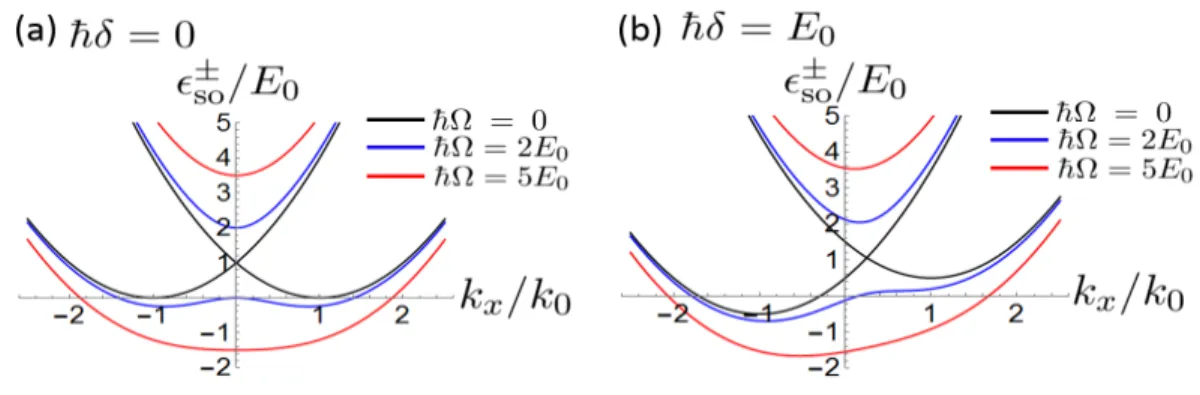
Figure 4.1: Dispersioins (4.2) in the kx direction. The lines are for ¯hΩ = 0 (black), 2E0

(Blue), and 5E₀ (Red) with (a) ¯hδ= 0 and (b) ¯hδ=E₀. The black and blue lines in Fig.

(a) show that the dispersion has two minima when δ= 0 and ¯hΩ<4E₀.

and plot this dispersion as a function of k_x in Fig. 4.1. When δ = 0, the ground state is doubly degenerated with nonzero momentum when Ω <4E0 (black and blue lines in Fig. 4.1(a)) and has zero momentum with no degeneracy when Ω ≥ 4E0

(red line in Fig. 4.1(a)), where these minima are given by

±k^min_δ=0 = (±k_δ=0^min,0,0), k_δ=0^min =





 k₀

√ 1−

(¯hΩ 4E₀

)2

(¯hΩ<4E₀) 0 (¯hΩ≥4E₀)

. (4.3)

When δ ̸= 0, on the other hand, the ground state has nonzero momentum with no degeneracy, where the minimum is given by k_δ^min_̸₌₀ = (k^min_δ_̸₌₀,0,0).

The eigen-state ˜ψ_±_,k satisfying ˜h_soψ˜_±_,k =ϵ^±_so(k) ˜ψ_±_,k can be written as (ψ˜_+,k

ψ˜₋_,k )

=

( cosθ_k_x sinθ_k_x

−sinθ_k_x cosθ_k_x

) (ψ˜_↑_,k ψ˜_↓_,k

)

, (4.4)

tanθ_k_x = 2

¯ hΩ



√(

−¯h²k₀k_x m +¯hδ

2 )2

+ (hΩ¯

2 )2

− ¯h²k₀k_x m +¯hδ

2



, (4.5)

where ˜ψk = ( ˜ψ_↑,k,ψ˜_↓,k)^T is the wave function of the boson with the wave number k (T denotes transpose). When δ = 0, since the ground state is doubly degenerated or is not degenerated, the ground state wave function in real space can be written as