Online Auction Markets
著者 HIROSE Yohsuke
journal or
publication title
明治学院大学経済研究 = The papers and proceedings of economics
volume 157
page range 123‑139
year 2019‑01‑31
URL http://hdl.handle.net/10723/00003546
1 Introduction
Today, many people use consumer-to-consumer electronic commerce sites to buy (or sell)
goods. In particular, with the emergence of online auction sites (e.g., eBay and Yahoo!), many people have become familiar with auctions. In such tradings, sellers often sell two or more items as bundling auctions. However, other sellers sell the same items separately. In this paper, we focus on bundling auctions of online auction markets. We propose an empirical model of online common value auctions for both bundling auctions and separate auctions.
Some papers focus on the bundling auction model in theoretical literature. Palfrey (1983) stud- ied bundling auctions with two bidders. He found that bundling auctions generate more expected revenues with two bidders within the private values paradigm. Chakraborty (1999) extended Pal- frey (1983) to a general number of bidders. He found that if the number of bidders grows large, the expected revenue of separate sales becomes greater than that of bundling auctions. While Chakraborty (1999) studied the private values model, Chakraborty (2002) studied the common value auction model and found the effect that they call the winner’s curse reduction effect in bundling auctions.
He also compared the expected revenues between bundling auctions and separate auctions.
Our empirical example involves eBay mint coin auctions in 2014. In our data set, there are two kinds of coin sets: 11-coin sets and 22-coin sets. We regard the 11-coin sets as separate items and the 22-coin sets as bundled items. We also conduct some counterfactual simulations using the estimated parameters. We evaluated the winner’s curse reduction effect in the sense of Chakraborty (2002)
and compared revenue between bundling auctions and separate auctions. Chakraborty (2002)
『経済研究』(明治学院大学)第 157 号 2019 年
An Empirical Analysis of Bundling Sales in Online Auction Markets
Yohsuke HIROSE
Faculty of Economics, Meijigakuin University
showed that bidders will bid more aggressively in separate auctions than in bundling auctions; he named this effect the winner’s curse reduction effect. We measured the magnitude of the winner’s curse reduction effect. We found that bidders in separate auctions will bid $2.5 higher than in bundling auc- tions. For revenue comparison, we found that the expected revenue in a bundling auction is higher than that in separate auctions by $0.37. Since the average transaction price of bundled items (22-coin sets) is $8.98, the value of additional gains are not negligible.
The rest of this paper is organized as follows. In Section 2, we describe the model of online auctions within the pure common value paradigm. Additionally, following Chakraborty (2002), we re- view the theoretical results for the bundling auctions. Section 3 describes the estimation strategy for the model described in Section 2. We utilize Bayesian estimation to estimate the structural parame- ters. In Section 4, we estimate the structural parameters using real auction data. Our empirical ex- ample is eBay mint coin set auctions in 2014. In Section 5, we compute the winner’s curse reduction effect in the sense of Chakraborty (2002) and compare the revenue between separate auctions and bundling auctions using the estimated parameters. Section 6 features some concluding remarks.
2 Model
There are N risk neutral potential bidders and a seller. The number of potential bidders, N, is a random variable and an exogenous variable. The seller sells two different objects k
=
1 and 2. In this model, we consider the pure common value model in which the ex post valuation of the item is the same for each bidder. Let V1 and V2 denote the values for items 1 and 2, respectively. The real- izations of values are unknown to the bidders. Instead, each bidder, i, receives her private signals corresponding to V1 and V2, which are denoted by S1i and S2i, respectively. Each bidder knows the realization of her own private signal but does not know the others’ before auctions. However, both the distribution of S1i and the distribution of S2i are common knowledge among bidders. In this paper, we consider a specific functional form for V1 and V2. We assume that the value of each item to bid- ders is the average of their signals. That is, the valuations take the form ofrespectively.1 For the bundled item, we impose the additive separability on bidder i’s signal for the bundled items, Si. Namely, we assume that Si
=
S1i+
S2i. Then, from our specific functional form for the value, the valuation of the bundled item, V, isWe assume that Sk1, …, SkNare independently and identically distributed. Namely, Ski ~i.i.d. N
i=1
∑
V1
=
N1 S1i andV2=
Ni=1
∑
S2i,1 N
N i=1
∑
V
=
N1 Si=
Ni=1
∑
(S1i+
S2i)=
V1+
V2N1
F(k x) for k
∈
{1, 2}. We assume that S1iand S2i are independently distributed. Furthermore, we as- sume that for each k∈
{1, 2}, Ski is affiliated with S1i+
S2i in the sense of Milgrom and Weber (1982).2.1 Equilibrium
In this paper, we regard online eBay auctions as second-price auctions. That is, each bidder submits her bid and the bidder with the highest bid among bidders wins the object and pays the second highest bid. Then, the equilibrium bidding strategies in separate auctions for items k
=
1 and2 are straightforward arguments from Milgrom and Weber (1982).
Let Yki be the highest signal except bidder i’s signal, Ski. That is, Yki
=
maxj≠i Skj. Then, the equilibrium bidding functions for bidder i with private signals S1i=
s1 and S2i=
s2 in separate auc- tions are given byb(1 s1)
=
E[V1|S1i=
s1, Y1i=
s1] and b(2 s2)=
E[V2|S2i=
s2, Y2i=
s2] (1)for items k
=
1 and 2, respectively.Analogously, the equilibrium bidding function for bundling auctions can be derived in the same manner. Let Si
=
S1i+
S2i be the sum of bidder i’s signals, S1i and S2i. Furthermore, let G(·) de- note the cumulative distribution function of Si=
S1i+
S2i. In other words, G(·) is the convolution of F(·) and 1 F(·). Then, 2 S1, …, SN are also independently and identically distributed with the CDF G(·).Namely, Si~i.i.d. G(s).
Let Yi be the highest signal except bidder i’s signal, Si. That is, Yi
=
maxj≠iSj. Then, using an argument similar to that of a separate auction, we gain the equilibrium bidding function for bidder i with signal Si=
s in the bundling auctionsb
(s)
=
E[V1+
V2|Si=
s, Yi=
s]. (2)2.2 Bundling auctions versus separate auction
Since we computed the various effects of bundling auctions in our empirical example, it is worth-while to review the theoretical result of bundling auctions within the common value paradigm.
Chakraborty (2002) discussed the bundling auctions model and the separate auctions model within the pure common value paradigm. Furthermore, he discussed the effect of bundling auctions and separate auctions with some useful examples. In this subsection, we review the results of Chakraborty (2002).
Chakraborty (2002) discussed that bundling auctions have a winner’s curse reducing effect.
The intuitive explanation of the winner’s curse reducing effect is as follows. In separate auctions of k
=
1 and 2, winning the items k=
1, 2 implies that each winner has the highest signal on each item.On the other hand, in a bundling auction, winning the bundled item implies that the winner has the highest signal for the bundled item but not for individual items, k
=
1 and 2. Therefore, winning thebundling auction is not as bad as winning two separate auctions. The following theorem is the Theo- rem 1 in Chakraborty (2002). They call the result of Theorem 1 the winner’s curse reducing effect.
Theorem 1 (Chakraborty (2002)). A bidder bids more aggressively when the objects are bundled.
That is,
b(s)
≥
b(1 s1)+
b(2 s2), where s=
s1+
s2.3 Estimation
The results of equilibrium bidding strategies (1) and (2) are familiar to economists. However, few empirical studies focus on the structural estimation of common value auction models. The main reason is the negative result of nonparametric identification on the common value auction model.
Athey and Haile (2002) and Athey and Haile (2007) showed the conditional distribution of Ski, given Vk is not identified from the observed bids in the common value auction model without additional identification conditions.
Therefore, most studies of structural estimation of the auction model focus on the private val- ues model. Recently, some papers have studied the identification condition of the common value auc- tion model. For example, Li, Perrigne, and Vuong (2000) showed the identification under the additive separability of the common value component. Février (2008) restricted the shape of the density function of the common value and showed the identification of the common value auction model.
d’Haultfoeuille and Février (2008) proposed the identification condition of the common value auction model, assuming the support of a private signal is finite and varies depending on the common value.
In this paper, we impose parametric specification to avoid the identification problem.
3.1 Estimation procedure
We observe Tk auctions indexed by t
=
1, …, Tk for item k∈
{1, 2}. The same items are each sold in separate auctions. Analogously, we observe T auctions indexed by t=
1, …, T for bundling auctions. We can observe each bidder’s bid, Bkit, and the number of actual bidders, nt, for bidder i, for item k∈
{1, 2}, and for auction t∈
{1, …, Tk }. We cannot observe each bidder’s signals, Skit and Sit, the common value, Vkt and Vt, and the number of potential bidders, Nt. We assume that the number of potential bidders is constant among auctions as is the maximum number of actual number of bidders observable by econometricians such as Guerre, Perrigne, and Vuong (2000).Following the example of Bajari and Hortaçsu (2003), we assume that bidders’ signals, Skit, are normally distributed with mean, µkt, and variance, σ2kt. That is, for k
∈
{1, 2}, Skit~
N(µkt, σ2kt), whereµkt
=
α’kXkt and σ2ktk=
(exp(βk1), …, exp(βkd))Xkt, where d represents the dimensionality of the vec- tor of the coefficient parameter, and Xkt is the vector of the auctionspecific covariate. The values of αk=
(αk1, …, αkd) and βk=
(βk1, …, βkd) are unknown to econometricians; therefore, we estimate these parameters.Recall that the equilibrium bidding function b(·) is given byk b(k sk)=E(Vkt|Skit
=
sk, Ykit=
sk).Since b(·) is a strictly increasing function, there exists an inverse function k ϕ(·). Note that since we k considered second-price auctions, the winning bid of item k,wkt, in auction t is the second-highest bid in auction t. Therefore, observing the winning bids, the likelihood function for separate auctions is given by
(3)
where f(·) is the probability density function of k Skit. In this case, f(·) is the normal density function.k The likelihood function for bundling auctions can be derived in the same manner. We assume that Sit is the normal random draw with mean µt and variance σ2t. That is, Sit~N (µt, σ2t) where µt
=
α’Xt and σ2t=(exp(β1), …, exp(βd))Xt, where α=
(α1, …, αd) and β=
(β1, …, βd) are the unknown coefficient parameter vector to be estimated.Since the equilibrium bidding function, b(·), is a strictly increasing function, there exists an in- verse function, ϕ(·). Similar to the separate auctions, since we considered second-price auctions, the winning bid, wt, in auction t is the second-highest bid in auction t. Therefore, in observing the win- ning bids, the likelihood function for the bundling auction is given by
(4)
where ɡ(·) is the probability density function of Sit. In this case, ɡ(·) is the normal density function.
t=1
Tk
∏ (1 1 N N-2) [
F(k ϕ(k wkt)|μkt, σ2kt)]
N-2L(w1, …, wkt|
α
k,β
k(, Xk1, …, Xkt))=
1 b(′k ϕ(k wkt))
×
f(k ϕ(k wkt)|μkt, σ2kt)× [
1-
F(k ϕ(k wkt)|μkt, σ2kt)]
,t=1
∏
T(
1 1 N N-
2) [G(ϕ(wt)|μt, σ2t)]
N-2
L(w1, …, wt|
α
,β
,(X1, …, Xt))=
1 b(′ ϕ(wt))
×
ɡ(ϕ(wt)|μt, σ2t)× [
1-
G(ϕ(wt)|μkt,σ2kt)]
,4 Empirical examples 4.1 Data description
Our empirical example consists of auctions of 2005 U.S. mint coin set held on eBay in 2014.
Data were collected from 208 eBay auctions completed in October, 2014. There are two types of goods in our data set. One is the 11-coin mint set and the other is the 22-coin mint set. The 22-coin mint set includes two packages of the 11-coin mint set. The sample sizes are 107 and 101, respectively.
As Bajari and Hortaçsu (2003) and Wegmann and Villani (2011) studied coin auctions in their empirical illustrations, coin auctions are excellent examples in the empirical study of the common values auction model. While Bajari and Hortaçsu (2003) and Wegmann and Villani (2011) both col- lected various kinds of coins in their empirical illustrations, we only collected 2005 U.S. mint coin sets
(11-coin sets and 22-coin sets). Therefore, we estimated the distribution of signals with fewer co- variates.
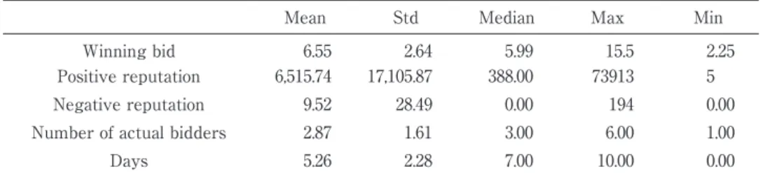
Tables 1 and 2 provide the summary of statistics for the 11-coin set and 22-coin set, respec- tively. The first column describes the variables. “Winning bid” is the second highest bid in the eBay auction. As seen in Tables 1 and 2, on average, one could purchase a mint coin set for $7.3 or $9.2 for the 11 -coin set or 22 -coin set, respectively. “Positive reputation” denotes the number of positive ratings a seller has received. Similarly, “Negative reputation” is the sum of the number of negative ratings and the number of neutral ratings a seller receives. Since the number of neutral ratings and the number of negative ratings are usually small relative to the number of positive ratings, we
Mean Std Median Max Min
Winning bid 8.98 3.35 8.25 17.0 3.3
Positive reputation 22,553.29 33,006.16 1,303.00 73,892.00 0.00
Negative reputation 13.39 17.17 3.00 57.00 0.00
Number of actual bidders 3.47 2.04 3.00 7.00 1.00
Days 5.98 2.06 7.00 10.00 1.00
Table 2: Summary statistics (2005 U.S. mint coin sets, (22-coin set) # of obs. = 101)
Mean Std Median Max Min
Winning bid 6.55 2.64 5.99 15.5 2.25
Positive reputation 6,515.74 17,105.87 388.00 73913 5
Negative reputation 9.52 28.49 0.00 194 0.00
Number of actual bidders 2.87 1.61 3.00 6.00 1.00
Days 5.26 2.28 7.00 10.00 0.00
Table 1: Summary statistics (2005 U.S. mint coin sets, (11-coin set) # of obs. =107)
regard neutral ratings as negative ratings. “Number of actual bidders” is the number of participants who actually bid at auction t. “Days” denotes the duration of the auctions held.
4.2 Estimation results 4.2.1 The 11-coin set
For the 11-coin set, we assume that the signal, Si, follows the normal distribution. That is, Sit~i.i.d. N(µ1t, σ21t ),
where µ1t
=
α0+
α1Xt1+
α2Xt2, and σ21t=
exp(β0)+
exp(β1)Xt1+
exp(β2)Xt2. The parameters α=
(α0, α1, α2) and β=
(β0, β1, β2)are unknown to econometricians.2 In this empirical illus- tration, the auction- specific covariates, Xt=
(Xt1, Xt2) are the logarithm of “Positive reputation+
1” and “Negative reputa- tion+
1”; that is,Xt1
=
log(Positive reputation+
1) and Xt2=
log(Negative reputation+
1)for observed auction t.
The prior distribution of α and β are α~N(0, 10I) and β~N(0, 10I), where I is the identity matrix of order 3.
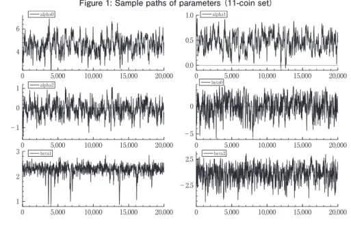
We used the random walk-based Metropolis-Hastings algorithm to generate random draws from the posterior distributions. The number of iteration is 20000, and the burn-in period is 1000. Ta- ble 3 reports the probabilities parameters take positive (PP), the p-values of convergence diagnos- tics for the MCMC (CD) and Inefficiency Factors (IF). All p-values of the convergence diagnostics are more than 0.06. Furthermore, the inefficiency factor values are sufficiently low. In particular, the inefficiency factors are 39.88 to 95.65, which implies that we would obtain the same variance of the posterior sample means from 209 uncorrelated draws, even in the worst case. Figure 1 shows the sample paths of estimated parameters. From Figure 1 it can be seen that the sample paths of these parameters converge to posterior distributions. Thus, we conclude that the sample paths of estimat- ed parameters converge to posterior distributions.
Figure 2 shows the posterior densities of parameters for the 11-coin set. Table 4 and Figure 2
Parameter Covariate (Coefficient Parameter) PP CD IF
µ1 Const. (α0) 1.00 0.77 87.41
log(Pos.Rep. +1)(α1) 1.00 0.85 95.65 log(Neg.Rep. +1)(α2) 0.46 0.96 66.27
σ21 Const. (β0) 0.51 0.06 54.85
log(Pos.Rep. +1)(β1) 1.00 0.32 47.15 log(Neg.Rep. +1)(β2) 0.44 0.77 39.88 Table 3: The convergence diagnostics for the MCMC (CD) and the inefficiency factors (IF) for the
11-coin set
Parameter Covariate (Coefficient Parameter) Mean Stdev. 95% credible interval
µ1 Const. (α0) 4.59 0.71 (3.23, 6.00)
log(Pos.Rep. +1) (α1) 0.46 0.17 (0.12, 0.79)
log(Neg.Rep. +1) (α2) −0.03 0.39 (−0.78, 0.73)
σ21 Const. (β0) 0.01 1.76 (−3.56, 3.12)
log(Pos.Rep. +1) (β1) 2.27 0.22 (1.71, 2.60)
log(Neg.Rep. +1) (β2) −0.35 1.60 (−3.70, 2.44)
Table 4: Posterior inferences for the 11-coin set Figure 1: Sample paths of parameters (11-coin set)
0 5,000 10,000 15,000 20,000
4 6
alpha0
0 5,000 10,000 15,000 20,000
0.0 0.5
1.0 alpha1
0 5,000 10,000 15,000 20,000
-1 0
1 alpha2
0 5,000 10,000 15,000 20,000
-5 0
beta0
0 5,000 10,000 15,000 20,000
1 2
3 beta1
0 5,000 10,000 15,000 20,000
-2.5
2.5 beta2
Figure 2: Posterior densities (11-coin set)
2 3 4 5 6 7
0.25 0.50
Density
alpha0
0.00 0.25 0.50 0.75 1.00 1
2 Density
alpha1
-1.5 -1.0 -0.5 0.0 0.5 1.0 1.5 0.5
1.0 Density
alpha2
-5.0 -2.5 0.0 2.5 5.0
0.1 0.2 Density
beta0
0.5 1.0 1.5 2.0 2.5 3.0
1 2 Density
beta1
-5.0 -2.5 0.0 2.5
0.1 0.2 Density
beta2
provide some posterior inferences. In Table 4, “Mean,” “Stdev,” and “95% interval” represent the pos- terior mean, the posterior standard deviation, the 95% credible interval, respectively.
As seen in Table 4, the posterior mean of α0 is 4.59. Since α0 is the constant term correspond- ing to the mean parameter µ1, when a seller has no reputation (i.e., a new entrant), the mean of the bidders’ signal is $4.59. As seen in Table 4, the posterior mean of α1 is 0.46, which is the coefficient parameter of the covariate log(Positive reputation
+
1) corresponding to the mean parameter µ1. Therefore, if a seller earns a more positive reputation, the mean of the bidders’ signals will increase.This result seems intuitively plausible. The posterior mean of α2 is
−
0.03, and α2 takes a positive val- ue with probability 0.46. Since α2 is the coefficient parameter of the covariate log(Negative reputa- tion+
1) corresponding to the mean parameter µ1, the number of negative ratings does not have much effect on the mean of the bidder’s signal. This result is not intuitively plausible. One possible reason for the tiny effect of negative reputations on the mean of bidders’ signals is the positive corre- lation between positive reputations and negative reputations. The correlation coefficient between positive reputations and negative reputations is 0.86 , which represents a high positive correlation.From Table 1, the number of negative ratings is small relative to the number of positive ratings.
There are very few auctions in which sellers receive negative ratings. In most cases, sellers receive positive ratings. Many sellers with log(Positive reputation
+
1)<
7(i.e., sellers with positive reputa- tions, less than 1100 total) had no negative ratings. All sellers with log(Positive reputation+
1)≥
7had some negative ratings.
Therefore, sellers with more trades receive more (both positive and negative) ratings. From these facts, we conclude that the number of negative ratings does not represent the insincerity of seller but, rather, the abundance of the seller’s experience, in our empirical example.
4.2.2 The 22-coin set
Similar to the case of 11-coin set, we assume that the signal Si follows the normal distribution.
That is,
Sit~i.i.d. N(µt, σ2t),
where µt
=
α0+
α1Xt1+
α2Xt2, and σ2t=
exp(β0)+
exp(β1)Xt1+
exp(β2)Xt2. The parameters α=
(α0, α1, α2) and β=
(β0, β1, β2 ) are unknown to econometricians. In this empirical illustration, the auction-spe- cific covariates, Xt=
(Xt1, Xt2) are the logarithm of “Positive reputation+
1” and “Negative reputa- tion+
1”.The prior distribution of α and β are α~N(0, 100I) and β~N(0, 100I), where I is the identi- ty matrix of order 3.
Similar to the case of 11-coin set, we use the random walk-based MH algorithm to generate random draws from the posterior distributions. We draw 30000 random samples from the posterior distribution via MH algorithm for each parameter. The burn-in period is 3000.
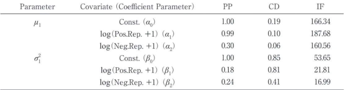
Table 5 provides the summary of statistics of posterior distributions and the p-values of con- vergence diagnostics for the MCMC (CD) and Inefficiency Factors (IF). All p-values of the conver- gence diagnostics are more than 0.06. Furthermore, the inefficiency factors are less than 188. There- fore, we would obtain the same variance of the posterior sample means from 159 uncorrelated draws, even in the worst case. Figure 3 shows the sample paths of estimated parameters. We conclude that the sample paths of estimated parameters converge to posterior distributions.
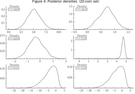
Figure 4 shows the posterior densities of parameters for the 22-coin set. Table 6 and Figure 4 provide some posterior inferences. As seen in Table 6, the posterior mean of α0 is 5.15. Since α0 is the constant term corresponding to the mean parameter µ. Therefore, when a seller has no reputation
(i.e., a new entrant), the mean of the bidders’ signal will be $5.15. The posterior mean of α1 is 0.70.
Since α1 is the coefficient parameter of the covariate log(Positive reputation
+
1) corresponding to the mean parameter µ, we find that positive reputation has positive effect on the mean of bidders’ sig- nals. The posterior mean of α2 is−
0.28 and α2 takes a positive value with probability 0.30. Recall thatParameter Covariate (Coefficient Parameter) PP CD IF
µ1 Const. (α0) 1.00 0.19 166.34
log(Pos.Rep.
+
1) (α1) 0.99 0.10 187.68 log(Neg.Rep. +1) (α2) 0.30 0.06 160.56σ21 Const. (β0) 1.00 0.85 53.65
log(Pos.Rep. +1) (β1) 0.18 0.81 21.81 log(Neg.Rep. +1) (β2) 0.24 0.41 16.99 Table 5: The convergence diagnostics for the MCMC (CD) and the inefficiency factors (IF) for the
22-coin set
Figure 3: Sample paths of parameters (22-coin set)
0 5,000 10,000 15,000 20,000 25,000 30,000 2.5
5.0 7.5
10.0 alpha0
0 5,000 10,000 15,000 20,000 25,000 30,000 0
1
alpha1
0 5,000 10,000 15,000 20,000 25,000 30,000
-1 0
1 alpha2
0 5,000 10,000 15,000 20,000 25,000 30,000 0.0
2.5
5.0 beta0
0 5,000 10,000 15,000 20,000 25,000 30,000
-20
-10
0 beta1
0 5,000 10,000 15,000 20,000 25,000 30,000
-10 0
beta2
α2 is the coefficient parameter of the covariate log(Negative reputation
+
1) corresponding to the mean parameter µ. According to our results, the number of negative ratings does not have much effect on the mean of bidders’ signals. This result is not plausible to our intuition. A possible reason is the same as in the case of 11-coin set. That is, a high positive correlation between positive reputa- tions and negative reputations. The correlation coefficient between positive reputations and negative reputations is 0.92, which represents a high positive correlation between positive reputations and negative reputations. Table 2 shows the number of negative ratings is small relative to the number of positive ratings. There are very few auctions in which sellers receive negative ratings. In most cases, sellers receive positive ratings. Analogous to the case of 11-coin set, Many sellers with log(Positive reputation
+
1)<
7.2 (i.e., sellers with positive reputations, less than 1330 total) had no neg- ative ratings. All sellers with log(Positive reputation+
1)≥
7 had some negative ratings. We conclude that the number of negative ratings does not represent the insincerity of seller but, rather, the abun- dance of the seller’s experience. As a result, negative ratings do not have much impact on the meanParameter Covariate (Coefficient Parameter) Mean Stdev. 95% credible interval
μ Const. (α0) 5.15 1.36 (2.53, 7.90)
log(Pos.Rep. +1) (α1) 0.70 0.29 (0.12, 1.25)
log(Neg.Rep. +1) (α2) −0.28 0.58 (−1.42, 0.89)
σ2 Const. (β0) 4.68 0.24 (4.27, 5.02)
log(Pos.Rep. +1) (β1) −3.56 3.79 (−12.37, 1.71)
log(Neg.Rep. +1) (β2) −3.18 3.94 (−12.21, 2.48)
Table 6: Posterior inferences for the 22-coin set
Figure 4: Posterior densities (22-coin set)
0.0 2.5 5.0 7.5 10.0
0.1 0.2 0.3 Density
alpha0
-0.5 0.0 0.5 1.0 1.5
0.5 1.0 1.5 Density
alpha1
-2 -1 0 1 2
0.25 0.50
0.75 Density
alpha2
0 1 2 3 4 5
1 2
Density
beta0
-25 -20 -15 -10 -5 0 5
0.05 0.10
Density
beta1
-25 -20 -15 -10 -5 0 5
0.05 0.10 Density
beta2
of bidders’ signals.
5 Counterfactual simulations
In this section, we compute the winner’s curse reduction effect in the sense of Chakraborty
(2002) and compare the revenue of separate auctions and bundling auctions using the estimated pa- rameters from Section 4.3
In our empirical model, the distribution of bidders’ signals depends on auction-specific covari- ates. We compute the winner’s curse reduction effect and the expected revenue for a “representa- tive” auction using the sample means of covariates, log(Positive reputation
+
1) and log(Negative reputation+
1), in Tables 1 and 2 and the posterior mean of the estimated parameters in Tables 4 and 6. The sample means of log(Positive reputation+
1) and log(Negative reputation+
1) arelog(Positive reputation
+
1)=
6.77 and log(Negative reputation+
1)=
1.34,respectively. The number of participants for a representative auction is N
=
7. Subsequently, the bid- ding functions can be computed using equations (1) and (2).In our empirical example, since the separate items, k
=
1 and k=
2, are the same item, we can- not estimate the parameters for item k=
2 directly. In other words, we cannot obtain the estimates for coefficient parameters (α, β) for item 2 from observed bids. However, for an arbitrary fixed co- variates (and hence for the representative auction), the distribution of bidders’ signals for item 2 can be identified. Since bidder i’s private signal for item k=
1, S1i, and bidder i’s private signal for item k=
2, S2i, are independent, the distribution of bidders’ signals for item 2 can be recovered from the identified distributions of bidders’ signals for item 1 , S1i, and bidders’ signals for bundled item, Si. Note that while we assume the independence, we do not assume that S1i and S2i have identical distri- butions.Since our parametric specification imposes that S1i, S2i, and Si are normal random variables, from the reproductive property of normal distributions, we have S2i~N(µ
−
µ1, σ2−
σ21), where (µ, σ2) and (µ1, σ21) are the parameters for distributions of Si and S1i, respectively. Let (µ2, σ22) be the parameter vector for distributions of S2i. By the estimated parameters and the sample mean of co- variates, we gain µ2=
1.85 and σ22=
40.53. Note that, since the mean of the signals for item 1 is µ1=
7.66, E(S1i)>
E(S2i) holds. This inequality seems intuitively plausible because the willingness to pay for the second item is usually less than that for the first item.The statement of Theorem 1 is the winner’s curse reduction effect, as proposed by Chakraborty (2002). Namely, b(i s)
≥
b1(i s1)+
b2(i s2). For each fixed signal s=
5, 10, 15, varying the value of the signal for item 1, s1, from 3.0 to s, we compute b(i s)−
(b1(i s1)+
b2(i s2)).Figures 5, 6, and 7 report the difference of the bidding function b(i s)
−
(b1(i s1)+
b2(i s2)) forfixed signals s
=
5, 10, 15, respectively. The shape of the graph with s=
5 is not similar to that of the graphs with s=
10, 15. When s=
5, the difference decreases as the signal for item 1, s1, increases. On the other hand, when s=
10 and 15, the difference decreases for s1∈
(3.0, 8.0) and s1∈
(3.0, 11.0) and it increases for s1>
8.0 and s1>
11.0, respectively. The values of b(i s)−
(b1(i s1)+
b2(i s2)) for s=
5, 10,15 are similar, around $2.50.
One may mistakenly conclude that Theorem 1 implies the revenue of bundling auctions is higher than that of separate auctions. Actually, Theorem 1 does not imply revenue ranking. In Theo-
Figure 5: Difference of the bidding function with s=5
3.0 3.2 3.4 3.6 3.8 4.0 4.2 4.4 4.6 4.8 5.0
2.352.362.372.382.392.402.412.422.43
Signal s1
Difference
B(is)-B1(is1)+B2(is2))
Figure 6: Difference of the bidding function with s=10
3.0 3.5 4.0 4.5 5.0 5.5 6.0 6.5 7.0 7.5 8.0 8.5 9.0 9.5 10.0
2.42.52.62.72.82.9
Signal s1
Difference
B(is)-B1(is1)+B2(is2))
rem 1, for any signal of bundling auctions, Si
=
s, the equation s=
s1i+
s2i must hold. When we compare the revenues, the equation s=
s1i+
s2i need not hold. The realizations of S1i and S2i are determined in- dependently.The expected revenues are computed by the Monte Carlo simulation method. Using the esti- mated parameters and the sample means of covariates, we draw the signals of bundling and separate auctions from the estimated distributions. We assume that the number of potential bidders is N
=
7.Then, the equilibrium bids for signals are computed via equation (1) and (2). The winning bids are the second-highest bids for both bundling and separate auctions. The revenue difference is computed by the difference between the bundling auction’s winning bid and that of the separate auction. We iterate this procedure 5000 times.
The density of revenue differences between bundling and separate auctions is shown in Figure 8. The shape of the density is symmetrical at point 0. Table 7 reports the summary statistics of revenues and revenue differences. In Table 7, “Mean” and “Stdev.” are the mean and the standard deviation of revenue differences, respectively. Similarly, “.25 quantile,” “Median,” and “.75 quantile”
represent the first quartile, the second quartile, and the third quartile. The probability that the revenue of bundling auctions is higher than that of separate auctions is denoted by “PP.”
According to Figure 8 and Table 7, the revenue of bundling auctions is higher than that of separate auctions with probability 0.53. The expected revenue difference is $0.37. Therefore, sellers can gain an additional profit of $0.37 by using a bundle auction rather than two separate auctions.
Since the average transaction price of bundled items (22-coin sets) is $8.98, we find that the value of additional gains are not negligible. In the theoretical literature, Chakraborty (2002) discussed the
Figure 7: Difference of the bidding function with s=15
3 4 5 6 7 8 9 10 11 12 13 14 15
2.502.753.003.253.503.75
Signal s1
Difference
B(is)-B1(is1)+B2(is2))
revenue ranking between the revenue of bundling auctions and separate auctions. He found that bundling auctions generate more expected revenue than do separate auctions when the number of bidders is sufficiently small. According to Tables 1 and 2, the number of participants at most 7.
Therefore, our empirical example does not contradicts the result of Chakraborty (2002).
6 Conclusions
In this paper, we focused on bundling auctions in online auction markets. In online auction markets (e.g., eBay and Yahoo!), sellers often sell two or more items in bundling auctions. Converse- ly, other sellers sell the same items separately. We propose an estimation procedure for bundling auction models within the pure common value paradigm.
Our empirical example is eBay mint coin set auctions in 2014. In our data set, there are two kinds of coin sets: 11-coin sets and 22-coin sets. We regard the 11-coin sets as the separate item and the 22-coin set as the bundled item. We also conducted some counterfactual simulations using the es- timated parameters. We computed the winner’s curse reduction effect following Chakraborty (2002)
Mean Stdev. .25 quantile Median .75 quantile PP
Revenue (bundle) 8.67 3.12 6.61 8.85 10.88 ―
Revenue (item 1) 6.99 2.48 5.39 7.10 8.73 ―
Revenue (item 2) 1.32 1.90 0.09 1.41 2.67 ―
Revenue difference 0.37 4.47 −2.60 0.38 3.40 0.53
Table 7: Summary statistics of revenue and revenue differences
Figure 8: Density of revenue difference between bundling auctions and separate auctions
-17.5 -15.0 -12.5 -10.0 -7.5 -5.0 -2.5 0.0 2.5 5.0 7.5 10.0 12.5 15.0 17.5 20.0
0.010.020.030.040.050.060.070.08
Revenue difference
Density
Density
Revenue Difference
precedent and compared the revenue of bundling auctions and separate auctions. We found that the value of the winner’s curse reduction effect is about $2.5. For revenue comparison, we found that the expected revenue in the bundling auctions is higher than that in the separate auctions by $0.37.
Since the average transaction price of bundled items (22-coin sets) is $8.98, the value of additional gains are not negligible.
There are some avenues for future research in this paper. For one, we ignored the endoge- nous entry of bidders. In general, bidders will decide endogenously to participate, whether in bun- dling auctions or separate auctions. Analogously, we also ignored the seller’s incentive to decide which item (the bundled item or separate items) to sell. The seller’s decision as to which item to sell will depend on the revenue ranking between bundling auctions and separate auctions.
Acknowledgment
I am indebted to Yasuhiro Omori for his warm encouragement and detailed comments. I am also grateful to Jun Nakabayashi and seminar participants at the 2014 Japanese Economic Associa- tion Autumn Meeting at Seinan Gakuin University for helpful comments and disscussions. The com- putational results are obtained by using Ox version 7.00 (Doornik (2007)).
Notes
1 This specification is the special case of Chakraborty (2002) and has been used in several papers. Example are Goeree and Offerman (2002) for auctions within common value and private values paradigm and Shahriar
(2008) and Shahriar and Wooders (2011) for auctions with buy prices model.
2 We omit subscript k
=
1 for the coefficient parameters α and β.3 Chakraborty (2002) also discussed the expected revenues of both bundling auctions and separate auctions.
Under the regularity conditions that are satisfied in our parametric specifications (i.e., normally distributed sig- nals), He found that revenue ranking between the revenue of bundling auctions and separate auctions depends on the number of potential bidders, N. He found that bundling auctions generate more expected revenue than do separate auctions for all N
<
N*, where N* is a sufficiently small number.References
Athey, Susan and Philip A. Haile. 2002. “Identification of Standard Auction Models.” Econometrica 70(6): 2107–
2140.
———. 2007 . “Nonparametric Approaches to Auctions.” In Handbook of Econometrics, vol. 6 A, edited by James Heckman and Edward Leamer. Amsterdam: Elsevier Science, 3847–3965.
Bajari, Patrick and Ali Hortaçsu. 2003. “The Winner’s Curse, Reserve Prices, and Endogenous Entry: Empirical Insights from eBay Auctions.” Rand Journal of Economics 34(2): 329–355.
Chakraborty, Indranil. 1999. “Bundling Decisions for Selling Multiple Objects.” Economic Theory 13(3): 723–733.
———. 2002. “Bundling and the Reduction of the Winner’s Curse.” Journal of Economics and Management Strategy 11(4): 663–684.
d’Haultfoeuille, Xavier and Philippe Février. 2008. “The Nonparametric Econometrics of Common Value Models.”
Working Paper.
Doornik, Jurgen A. 2007. Object-Oriented Matrix Programming Using Ox. London: Timberlake Consultants Press, 3rd ed.
Février, Philippe. 2008. “Nonparametric Identification and Estimation of a Class of Common Value Auction Mod- els.” Journal of Applied Econometrics 23(7): 949–964.
Goeree, Jacob K. and Theo Offerman. 2002. “Efficiency in Auctions with Private and Common Values: An Exper- imental Study.” American Economic Review 92(3): 625–643.
Guerre, Emmanuel, Isabelle Perrigne, and Quang Vuong. 2000. “Optimal Nonparametric Estimation of First-Price Auctions.” Econometrica 68(3): 525–574.
Li, Tong, Isabelle Perrigne, and Quang Vuong. 2000 . “Conditionally Independent Private Information in OCS Wildcat Auctions.” Journal of Econometrics 98(1): 129–161.
Milgrom, Paul R. and Robert J. Weber. 1982. “A Theory of Auctions and Competitive Bidding.” Econometrica 50
(5): 1089–1122.
Palfrey, Thomas R. 1983 . “Bundling Decisions by a Multiproduct Monopolist with Incomplete Information.”
Econometrica 51(2): 463–483.
Shahriar, Quazi. 2008. “Common Value Auctions with Buy Prices.” Working Paper.
Shahriar, Quazi and John Wooders. 2011. “An Experimental Study of Auctions with a Buy Price under Private and Common Values.” Games and Economic Behavior 72(2): 558–573.
Wegmann, Bertil and Mattias Villani. 2011. “Bayesian Inference in Structural Second-Price Common Value Aauc- tions.” Journal of Business & Economic Statistics 29(3): 382–396.