The mean field analysis of the Kuramoto model on graphs II. Asymptotic stability of the incoherent state, center manifold reduction, and bifurcations

The mean field analysis of the Kuramoto model on graphs II.

Asymptotic stability of the incoherent state, center manifold reduction, and bifurcations

Hayato Chiba

^∗

and Georgi S. Medvedev

^†

September 25, 2017

Abstract

In our previous work [3], we initiated a mathematical investigation of the onset of synchronization in the Kuramoto model (KM) of coupled phase oscillators on convergent graph sequences. There, we derived and rigorously justified the mean field limit for the KM on graphs. Using linear stability analysis, we identified the critical values of the coupling strength, at which the incoherent state looses stability, thus, determining the onset of synchronization in this model.

In the present paper, we study the corresponding bifurcation. Specifically, we show that similar to the original KM with all-to-all coupling, the onset of synchronization in the KM on graphs is realized via a pitchfork bifurcation. The formula for the stable branch of the bifurcating equilibria involves the principal eigenvalue and the corresponding eigenfunctions of the kernel operator defined by the limit of the graph sequence used in the model. This establishes an explicit link between the network structure and the onset of synchronization in the KM on graphs. The results of this work are illustrated with the bifurcation analysis of the KM on Erd˝os-R´enyi, small-world, as well as certain weighted graphs on a circle.

1 Introduction

In 1970s, a prominent Japanese physicist Yoshiki Kuramoto described a remarkable effect in collective dy- namics of large systems of coupled oscillators [11]. He studied all-to-all coupled phase oscillators with randomly distributed intrinsic frequencies, the model which now bears his name. When the strength of cou- pling is small, the phases are distributed approximately uniformly around a unit circle, forming an incoherent state. Kuramoto identified a critical value of the coupling strength, at which the the incoherent state looses stability giving rise to a stable partially synchronized state. To describe the bifurcation corresponding to the onset of synchronization, Kuramoto introduced the order parameter - a scalar function, which measures the

∗Institute of Mathematics for Industry, Kyushu University / JST PRESTO, Fukuoka, 819-0395, Japan, [email protected]

degree of coherence in the system. He further showed that the order parameter undergoes a pitchfork bifur- cation. Thus, the qualitative changes in the statistical behavior of a large system of coupled phase oscillators near the onset to synchronization can be described in the language of the bifurcation theory.

Kuramoto’s discovery created a new area of research in nonlinear science [20, 21, 19]. The rigorous mathematical treatment of the pitchfork bifurcation in the KM was outlined in [4] and was presented with all details in [1]. The analysis in these papers is based on the generalized spectral theory for linear operators [2] and applies to the KM with intrinsic frequencies drawn from a distribution with analytic or rational probability density function. Under more general assumptions on the density, the onset of synchronization in the KM was analyzed in [6, 8, 5]. These papers use analytical methods for partial differential equations and build upon a recent breakthrough in the analysis of Landau damping [18].

In our previous work [3], we initiated a mathematical study of the onset of synchronization in the KM on graphs. Following [14, 15], we considered the KM on convergent families of deterministic and random graphs, including Erd˝os-R´enyi and small-world graphs among many other graphs that come up in appli- cations. For this model, we derived and rigorously justified the mean field limit. The latter is a partial differential equation approximating the dynamics of the coupled oscillator model in the continuum limit as the number of oscillators grows to infinity. In [3], we performed a linear stability analysis of the incoherent state and identified the boundaries of stability. Importantly, we related the stability region of the incoherent state to the structural properties of the network through the spectral properties of the kernel operator defined by the limit of the underlying graph sequence [12]. In the present paper, we continue the study initiated in [3]. Here, we analyze the bifurcations at the critical values of the coupling strength, where the incoherent state looses stability. In the remainder of this section, we review the model and the main outcomes of [3]

and explain the main results of this work.

We begin with a brief explanation of the graph model that was used in [3] and will be used in this paper.

In [3], we adapted the construction of W-random graphs [13] to define a convergent sequence of graphs. The flexible framework of W-random graphs allows us to deal with a broad class of networks that are of interest in applications. Let W be a symmetric measurable function on the unit square I

²

:= [0, 1]

²

with values in [−1, 1] and let X

n

= {ξ

_n1

, ξ

n2

, . . . , ξ

nn

} form a triangular array of points ξ

ni

, i ∈ [n] := {1, 2, . . . n}, n ∈ N , subject to the following condition

n→∞

lim n

⁻¹

n

X

i=1

f (ξ

_ni

) = Z

I

f(x)dx ∀f ∈ C(I). (1.1)

Γ

n

= hV (Γ

n

), E (Γ

n

), (W

nij

)i is a weighted graph on n nodes labeled by the integers from [n], whose edge set is

E(Γ

_n

) = {{i, j} : W (ξ

_ni

, ξ

_nj

) 6= 0, i, j ∈ [n]} .

Each edge {i, j} ∈ E(Γ

n

) is supplied with the weight W

nij

:= W (ξ

ni

, ξ

nj

). In the theory of graph limits, W is called a graphon [12]. It defines the asymptotic properties of {Γ

_n

} for large n.

Consider the initial value problem (IVP) for the KM on Γ

_n

θ ˙

ni

= ω

i

+ Kn

⁻¹

n

X

j=1

W

nij

sin(θ

nj

− θ

ni

), i ∈ [n], (1.2)

θ

ni

(0) = θ

⁰_ni

. (1.3)

The intrinsic frequencies ω

_i

, i ∈ [n], are independent identically distributed random variables. The dis- tribution of ω

1

has density g(ω). For the spectral analysis in Section 3, we need to impose the following assumptions on g: a) g : R → R

⁺

∪ {0} is an even unimodal function, and b) g is real analytic function with finite moments of all orders: R

R

|x|

^m

g(x)dx < ∞, m ∈ N. For instance, the density of the Gaussian distri- bution satisfies these conditions. The KM on weighted graphs {Γ

_n

} (1.2), (1.3) can be used to approximate the KM on a variety of random graphs (cf. § 4.2 [3]).

Along with the discrete model (1.2) we consider the IVP for the following partial differential equation

∂

∂t ρ(t, θ, ω, x) + ∂

∂θ {ρ(t, θ, ω, x)V (t, θ, ω, x)} = 0, (1.4) ρ(0, θ, ω, x) = ρ

⁰

(θ, ω, x) ∈ S × R × I, (1.5) where

V (t, θ, ω, x) = ω + K Z

I

Z

R

Z

S

W (x, y) sin(φ − θ)ρ(t, φ, ω, y)g(ω)dφdωdy. (1.6) Here, ρ(t, θ, ω, x) is the conditional density of the random vector (θ, ω) given ω, and parametrized by (t, x) ∈ R

⁺

× I, and S = R/2πZ is a circle. In particular,

Z

S

ρ(t, θ, ω, x)dθ = 1 ∀(t, ω, x) ∈ R

⁺

× R × I. (1.7) It is shown in [3, Theorem 2.2] that

µ

ⁿ_t

(A) = n

⁻¹

n

X

i=1

δ

_{(θni(t),ωi,ξni)}

(A) (1.8) interpreted as a probability measure on Borel sets A ∈ B (G), G = S × R × I, converges in the bounded Lipschitz distance [7] uniformly on bounded time intervals to the absolutely continuous measure

µ

_t

(A) = Z

A

ρ(t, θ, ω, x)g(ω)dθdωdx, A ∈ B (G), (1.9) provided µ

ⁿ₀

and µ

0

are sufficiently close in the same distance. The latter can be achieved with the appro- priate initial condition (1.3) and sufficiently large n (see [3, Corollary 2.3]). Therefore, the IVP (1.4),(1.5) approximates the IVP (1.2),(1.3) on finite time intervals for sufficiently large n.

An inspection of (1.4) shows that ρ

u

= 1/(2π), the density of the uniform distribution on S , is a steady state solution of (1.4). It corresponds to the incoherent (mixing) state of the KM. Numerics suggests that the incoherent state is stable for small K ≥ 0. The loss of stability of the incoherent state is interpreted as the onset of synchronization in the KM. This is the main focus of [3] and of the present paper. In [3], we identified the boundaries of the region of stability of the incoherent state in (1.4). Specifically, we showed that there exist K

_c⁻

≤ 0 ≤ K

_c⁺

such that ρ

_u

is linearly stable for K ∈ [K

_c⁻

, K

_c⁺

], and is unstable otherwise.

The critical values K

_c⁻

and K

_c⁺

depend on the network topology through the eigenvalues of the compact symmetric operator W : L

²

(I) → L

²

(I)

Z

The eigenvalues of W are real with the only accumulation point at 0. Denote the largest positive and smallest negative eigenvalues of W by µ

max

and µ

min

respectively. If all eigenvalues are nonnegative (nonpositive), we set µ

_min

= −∞ (µ

_max

= ∞). The main stability result of [3] yields explicit expressions for the transition points

K

_c⁻

= 2

πg(0)µ

_min

and K

_c⁺

= 2

πg(0)µ

_max

. (1.11)

Thus, the region of linear stability of ρ

_u

depends explicitly on the spectral properties of the limiting graphon W . Recall that W represents the graph limit of {Γ

_n

}. Thus, (1.11) links network topology to synchroniza- tion in (1.2). For the classical KM (all-to-all coupling), W (x, y) = 1 and µ

min

= −∞, µ

_max

= 1, which recovers the known Kuramoto’s formula.

In the present paper, we study the onset of synchronization in (1.2) in more detail. After some prelimi- naries and preparatory work in Sections 2 and 3, we revisit linear stability of the incoherent solution. This time, we show that despite the lack of eigenvalues with negative real part and the presence of the continuous spectrum on the imaginary axis, the incoherent state is an asymptotically stable solution of the linearized problem (cf. Theorem 4.1). This is a manifestation of the Landau damping in the KM.

In Section 5, we study the bifurcation at K

_c⁺

with a one-dimensional center manifold. To this end, we recall the order parameter

h(t, x) = Z

I

Z

R

Z

S

W (x, y)e

^iθ

ρ(t, θ, ω, y)g(ω)dθdωdy, (1.12) which was introduced in [3] as a measure of coherence in the KM on graphs. This is a continuous analog of the local order parameter

1 n

n

X

j=1

W

nij

e

^iθnj(t)

for the discrete model (1.2). The order parameter generalizes the original order parameter used by Kuramoto for the all-to-all coupled model. Note that (1.12) depends on x and contains information about the structure of the network through W . As will be clear below, the order parameter plays an important role in the analysis of the mean field equation. In particular, it can be used to locate nontrivial steady state solutions. To this end note that the velocity field (1.6) can be conveniently rewritten in terms of the order parameter

V (t, θ, ω, x) = ω + K 2i

e

^−iθ

h(t, x) + e

^iθ

h(t, x)

. (1.13)

In particular, for a given steady state of the order parameter written in the polar form

h

∞

(x) = R(x)e

^iΦ(x)

, (1.14)

the velocity field takes the following form

V (t, θ, ω, x) = ω − KR(x) sin(θ − Φ(x)).

Setting ∂

θ

(V ρ) = 0, we find the corresponding steady state solution of (1.4) ρ(θ, ω, x) =







δ θ − Φ(x) − arcsin(ω/KR(x))

, |ω| ≤ KR(x), 1

2π

p ω

²

− K

²

R(x)

²

|ω − KR(x) sin(θ − Φ(x))| , |ω| > KR(x), (1.15)

where δ stands for the Dirac delta function. The stationary solution (1.15) has the following interpretation:

the first line describes phase-locked oscillators, while the second line yields the distribution of the drifting oscillators. Thus, solutions of this form may combine phase-locked oscillators and those moving irregularly.

Such solutions are called partially phase-locked or partially synchronized. The phase of a phase-locked oscillator at x with a natural frequency ω, is given by

θ = Φ(x) + arcsin ω

KR(x)

, (1.16)

provided |ω| ≤ KR(x). In Sections 5 and 6, we will identify branches of stable equilibria bifurcating from K

_c^±

in terms of the corresponding values of the order parameter. Then Equation (1.16) will be used to describe the corresponding stable phase-locked solutions.

In Section 5, assuming that µ

max

is a simple eigenvalue of W, we show that the coupled system (1.2) un- dergoes a supercritical pitchfork bifurcation at K

_c⁺

. Specifically, we derive an ordinary differential equation for the order parameter h and show that the trivial solution of this equation looses stability at K

_c⁺

and gives rise to a stable branch of (nontrivial) equilibria, corresponding to partially synchronized state (cf. (5.1)). In Section 6, we consider the onset of synchronization in networks with certain symmetries (cf. (6.1)). This leads to the bifurcation with a two-dimensional center manifold. The bifurcation analysis in Sections 5 and 6 is illustrated with the analysis of the KM on Erd˝os-R´enyi, small-world graphs, and to a class of weighted graphs on a circle.

2 Preliminaries

In the remainder of this paper, we will assume that K ≥ 0. The case of negative K is reduced to that above by switching to K := −K and W := −W . Furthermore, without loss of generality we assume that µ

_max

> 0.

2.1 Fourier transform

We rewrite (1.4) in terms of the complex Fourier coefficients z

_j

=

Z

S

e

^ijθ

ρ(t, θ, ω, x)dθ, j ∈ Z . (2.1) Applying the Fourier transform to (1.4) and using integration by parts, we obtain

∂z

j

∂t = − Z

S

e

^ijθ

∂

∂θ {V (t, θ, ω, x)ρ(t, θ, ω, x)} dθ

= ij Z

S

e

^ijθ

V (t, θ, ω, x)ρ(t, θ, ω, x)dθ

= ijωz

_j

+ jK 2

Z e

^ijθ

e

^−iθ

h(t, x) − e

^iθ

h(t, x)

ρ(t, θ, ω, x)dθ,

(2.2)

where

h(t, x) = Z

I

Z

R

Z

S

W (x, y)e

^iθ

ρ(t, θ, ω, y)g(ω)dθdωdy

= Z

I

Z

R

W (x, y)z

1

(t, ω, y)g(ω)dωdy.

(2.3)

From (2.2), we further obtain

∂z

j

∂t = ijωz

_j

+ jK

2 hz

j−1

− hz

_j+1

, j ∈ Z . (2.4)

By (1.7), z

0

= 1. Further, z

−j

= ¯ z

j

, because ρ is real. Thus, in (2.4) we can restrict to j ∈ N.

Let

Pf(ω, x) = Z

R

W[f ](ω, x)g(ω)dω

= Z

I

Z

R

W (x, y)f (ω, y)g(ω)dωdy.

(2.5)

Combining these observations, we rewrite (2.4):

∂

∂t z

₁

= iωz

₁

+ K

2 Pz

₁

− Pz

₁

z

₂

, (2.6)

∂

∂t z

j

= ijωz

j

+ jK

2 Pz

1

z

j−1

− Pz

1

z

j+1

, j = 2, 3, . . . . (2.7)

Note that the trivial solution Z := (z

₁

, z

₂

, . . . ) ≡ 0 is a steady state solution of (2.6), (2.7). It corre- sponds to the uniform distribution ρ

_u

= 1/(2π), a constant steady state solution of (1.4). Linearizing around Z ≡ 0, we arrive at

∂

∂t z

₁

= Tz

₁

, (2.8)

∂

∂t z

_j

= ijωz

_j

, j = 2, 3, . . . , (2.9) where T is a linear operator on H := L

²

( R × I, g(ω)dωdx)

Tf = iωf + K

2 Pf. (2.10)

2.2 The eigenvalue problem

The multiplication operator M

_iω

: H → H defined by

M

_iω

f = iωf, ω ∈ R (2.11)

is a closed operator. The continuous spectrum of M

_iω

fills the imaginary axis

σ

_c

(M

_iω

) = isupp(g) = i R . (2.12) Since P is compact (as a Hilbert-Schmidt operator), T : H → H is closed and σ

c

(T) = i R .

Next we turn to the eigenvalue problem

Tf = λf, (2.13)

where T and P are operators on H (cf. (2.10) and (2.5)).

We will locate the eigenvalues of T through the eigenvalues of W (cf. (1.10)). Since W is a compact symmetric operator on L

²

(I ), it has a countable set of real eigenvalues with the only accumulation point at zero. All nonzero eigenvalues have finite multiplicity.

Suppose λ is an eigenvalue of T and v ∈ H is the corresponding eigenfunction. Then a simple calcula- tion yields (cf. [3])

w = K

2 D(λ)Ww, (2.14)

where

D(λ) = Z

R

g(ω)dω

λ − iω , (2.15)

w = Z

R

v(ω, ·)g(ω)dω ∈ L

²

(I ). (2.16) Equation (2.14) yields the equation for eigenvalues of T

D(λ) = 2

Kµ , (2.17)

where µ is a nonzero eigenvalue of W.

Using (2.17), we establish a one-to-one correspondence between the eigenvalues of W and those of T.

Specifically, for every positive eigenvalue of W, µ, there is a branch of eigenvalues of T, λ = λ(µ, K ), K ≥ K(µ) := 2

πg(0)µ , (2.18)

such that

K→K(µ)+0

lim λ(µ, K) = 0+, lim

K→∞

λ(µ, K) = ∞. (2.19)

Recall that µ

_max

stands for the largest positive eigenvalue of W. Then for K ∈ [0, K(µ

_max

)) there are no

eigenvalues with positive real part. Furthermore, for small ε > 0 and K ∈ (K(µ

max

), K (µ

max

) + ε) there

is a unique positive eigenvalue of T, λ(K, µ

_max

), which vanishes as K → K(µ

_max

) + 0 (see [3] for more

details).

3 The generalized spectral theory

The major obstacle in studying stability and bifurcations of the incoherent state is the continuous spectrum of the linearized problem on the imaginary axis (cf. (2.12)). To deal with this difficulty, we develop the generalized spectral theory following the treatment of the classical KM in [1]. Below, we outline the key steps in the analysis of the generalized eigenvalue problem referring the interested reader to [1] for missing proofs and further details.

3.1 The rigged Hilbert space

Here, we define the rigged Hilbert space which will be used in the spectral analysis below. Let Exp(β, n) be the set of holomorphic functions on the region C

n

:= {z ∈ C | Im(z) ≥ −1/n} such that the norm

||φ||

_β,n

:= sup

Im(z)≥−1/n

e

^−β|z|

|φ(z)| (3.1)

is finite. With this norm, Exp(β, n) is a Banach space [1]. Let Exp be their inductive limit with respect to n = 1, 2, . . . and β = 0, 1, 2, . . .

Exp = lim −→

β≥0

lim −→

n≥1

Exp(β, n) = [

β≥0

[

n≥1

Exp(β, n). (3.2)

With the inductive limit topology, Exp is a complete Montel space

¹

. The properties of Exp are described in detail in [1].

Next, we define X := Exp ⊗L

²

(I) as a topological tensor product of Exp and L

²

(I). X is a complete Montel space. It is a dense subspace of H. The topology of X is stronger than that of H. For every f ∈ X we have f (ω, ·) ∈ L

²

(I ) for each ω ∈ R . In addition, f (ω, x) is holomorphic in ω on the upper half plane, where it can grow at most exponentially.

Let X

⁰

be the dual space of X. It is the space of continuous antilinear functionals on X. Let h·, ·i denote the pairing between X

⁰

and X, i.e., for l ∈ X

⁰

and f ∈ X, hl, f i := l(f ) stands for the corresponding antilinear functional.

The dual space X

⁰

is equipped with the weak dual topology (cf. [1])

²

. H is a dense subspace of X

⁰

, and the topology of H is stronger than that of X

⁰

. Hence,

X ⊂ H ⊂ X

⁰

form a rigged Hilbert space (a.k.a. Gelfand triple) [10].

Note that if l ∈ X

⁰

∩ L

²

(R × I, g(ω)dωdx) then hl, f i := (l, f

^∗

)

_L2(R×I)

=

Z

I

Z

R

l(ω, x)f (ω, x)g(ω)dωdx,

1A locally convex topological vector space is called Montel if every bounded set in it is relatively compact.

2{ln} ⊂X⁰converges tol∈X⁰ifhln, fi ∈Ctends tohl, fifor everyf∈X.

for f ∈ X, where f

^∗

(ω, x) := f(ω, x). Thus, T and the rigged Hilbert space defined above satisfy all assumptions of the generalized spectral theory in [1].

3.2 The generalized eigenvalue problem

In this subsection we calculate the resolvent of T and spectral projections. With the rigged Hilbert space defined above, we will view the resolvent as an operator from X to X

⁰

.

Below, we will need to construct analytic continuation for certain functions involving integrals of Cauchy type. For this, we are going to use an implication of the Sokhotski formulas, which we formulate as a separate statement for convenience.

Lemma 3.1. (Sokhotski, cf. [9]) Let f be a complex valued function on R . Suppose f has at most a finite number of integrable discontinuities. Then

F (z) = Z

R

f (ω)dω

z − iω (3.3)

is an analytic function in the right and left open half-planes of C . Furthermore, for z = x +iy, the following formulas determine the limits of F (z) as x → 0±:

x→0±

lim F (z) = ±πf (y) + i PV Z

iR

f (−iφ)dφ φ − iy

= ±πf (y) − iπH [f ](y),

(3.4)

where PV stands for the principal value in the sense of Cauchy and H[f ] denotes the Hilbert transform of f .

Corollary 3.2. Suppose f is holomorphic on the real axis and admits the analytic continuation to the upper half-plane. Then

F ˜ (z) =







F (z), x > 0, lim

x→0+

F (z), x = 0, F (z) + 2πf(−iz), x < 0,

(3.5) is an entire function.

3.3 The generalized resolvent

Our next goal is to compute the resolvent of T

R(λ) = (λ − T)

⁻¹

. (3.6)

To this end, we first compute R(λ) for Re(λ) > 0 and extend it analytically to the left half-plane as an

operator from X to X

⁰

.

In the right half-plane Re(λ) > 0, R(λ) can be rewritten as follows R(λ) = A(λ)

I − K

2 PA(λ)

−1

, (3.7)

where

A(λ) = (λ − iω)

⁻¹

, (3.8)

and I stands for the identity operator. Note that A(λ) ceases to exist as the multiplication operator on H as Re(λ) → 0 (recall that the imaginary axis is the continuous spectrum of M

_iω

). However, it can be extended to the left half-plane as as an operator A : X → X

⁰

defined as follows

h A (λ)u, vi =







(A(λ)u, v

^∗

)

_H

, Re(λ) > 0,

lim

Re(λ)→0+

(A(λ)u, v

^∗

)

_H

, Re(λ) = 0,

(A(λ)u, v

^∗

)

_L2(R×I,gdωdx)

+ 2πg(−iλ) R

I

u(−iλ, x)v(−iλ, x)dx, Re(λ) < 0.

(3.9)

By Corollary 3.2, h A (λ)u, vi is an entire function in λ for all u, v ∈ X. This suggests an appropriate generalization of R(λ), R(λ) : X → X

⁰

defined by

R (λ) = A (λ)

I − K

2 P

^×

A (λ)

−1

, (3.10)

where P

^×

: X

⁰

→ X

⁰

is the dual operator of P.

For each u ∈ X, R (λ)u is an X

⁰

-valued meromorphic function. For Re(λ) > 0, it coincides with the restriction of R(λ) to X. Thus, R(λ) is a meromorphic continuation of R(λ) from the right half-plane to the left-half plane as an X

⁰

-valued operator. Note that since T has the continuous spectrum on the imaginary axis, R(λ) can not be continued to the left-half plane as an operator on H.

We define the generalized eigenvalues of T as the singularities of the generalized resolvent R(λ).

Definition 3.3. λ ∈ C is called a generalized eigenvalue of T if there is a nonzero v ∈ X

⁰

such that

I − K

2 P

^×

A (λ)

v = 0 (3.11)

In this case, v is called a generalized eigenfunction.

It turns out that the generalized eigenvalues and the corresponding eigenfunctions of T are, in fact, the eigenvalues and eigenfunctions of the dual of T, T

^×

.

Theorem 3.4. (cf. [2]) Let λ ∈ C be a generalized eigenvalue of T and v ∈ X

⁰

is the corresponding eigenfunction. Then T

^×

v = λv.

Remark 3.5. Using (3.9) and (3.11), one can see that the generalized eigenvalues λ = λ(µ, K ) of T are the roots of the following equation

2

Kµ = D (λ), (3.12)

where µ is a nonzero eigenvalue of W and D(λ) =



 

 

D(λ), Re(λ) > 0,

Re(λ)→0+

lim D(λ), Re(λ) = 0, D(λ) + 2πg(−iλ), Re(λ) < 0.

(3.13)

The right hand side of (3.13) is an entire function (cf. Corollary 3.2). For Re(λ) > 0, (3.12) is reduced to the equation for the eigenvalues of T (cf. (2.17)). In this case, the corresponding generalized eigenfunction v is included in L

²

( R × I, gdωdx), i.e., λ is an eigenvalue of T. On the other hand, for Re(λ) ≤ 0, the generalized eigenfunction v is not in H but is an element of the dual space X

⁰

.

3.4 The generalized Riesz projection

Let µ be a positive eigenvalue of W and w ∈ L

²

(I ) be the corresponding eigenfunction. The largest positive eigenvalue of W and the corresponding eigenfunction are denoted by µ

max

and w

max

respectively. For every K > K

_c⁺

= 2/(πg(0)µ

max

) there is a real positive eigenvalue of T, λ = λ(µ, K). The corresponding eigenfunction is given by

v(ω, x) = K 2

w(x)

λ − iω . (3.14)

As K approaches the critical value K

_c⁺

from above, the eigenvalue λ(µ

max

, K) converges to 0+ along the real axis and at K = K

_c⁺

it hits the continuous spectrum on the imaginary axis. The corresponding eigenfunction approaches the critical vector

X

⁰

3 v

⁺_c

:= K

_c⁺

2 lim*

λ→0+

w

max

λ − iω , (3.15)

where lim* stands for the limit in X

⁰

with respect to the weak dual topology, i.e., the action of v

⁺_c

∈ X

⁰

on u ∈ X is given by

hv

_c⁺

, ui = K

_c⁺

2 lim

λ→0+

Z

R×I

w

max

(x)g(ω)

λ − iω u(ω, x)dωdx

= K

_c⁺

2 lim

λ→0+

Z

R

(w

_max

, u

^∗

(ω, ·))

_L2(I)

g(ω)dω

λ − iω .

(3.16)

Let λ ∈ C be a generalized eigenvalue of T. Then the generalized Riesz projection Π

_λ

: X → X

⁰

is defined by

Π

λ

= 1 2πi

Z

γ(λ)

R(z)dz, (3.17)

where γ (λ) is a simple closed curve around λ oriented counterclockwise that does not encircle or intersect

the rest of the spectrum. Below, we shall refer to such curves as contours. The image of Π

_λ

gives the

generalized eigenspace of λ [1].

Theorem 3.6. Suppose the algebraic and geometric multiplicities of µ

_max

coincide. Then the generalized Riesz projection of λ = 0, the generalized eigenvalue of T for K = K

_c⁺

, has the following form

Π

0

= − lim*

λ→0+

D

⁰

(λ)

⁻¹

A(λ) ˜ Π

µmax

D(λ)

= g

₁

lim*

λ→0+

A(λ) ˜ Π

_µmax

D(λ) ,

(3.18)

where g

1

= − lim

λ→0+

D

⁰

(λ)

⁻¹

is a positive constant, A(λ) was defined in (3.8), and Π ˜

µ

stands for the Riesz projection onto the eigenspace of W corresponding to the eigenvalue µ. The operator D(λ) on H is defined by

D(λ)v = Z

R

v(ω, ·)g(ω)dω

λ − iω , v ∈ L

²

( R × I, gdωdx). (3.19) The proof of Theorem 3.6 relies on three technical lemmas. Below we state and prove these lemmas first and then prove the theorem.

Lemma 3.7. Let Re(λ) > 0 then R(λ)v = A(λ)v + K

2 A(λ)W

I − K

2 D(λ)W

−1

D(λ)v, v ∈ H. (3.20)

Proof. By definition of R(λ) (3.6), for any v ∈ H, we have

λ − iω − K 2 P

R(λ)v = v, and, thus,

R(λ)v = A(λ)v + K

2 A(λ)PR(λ)v. (3.21)

Using Fubini theorem, from (2.5) we have PR(λ)v = W

Z

R

(R(λ)v)(ω, ·)g(ω)dω

=: WQv.

(3.22)

On the other hand, integrating both sides of (3.21) against g(ω)dω, we obtain Qv =

Z

R

(R(λ)v)(ω, ·)g(ω)dω

= D(λ)v + K 2 D(λ)

Z

R×I

W (·, y) (R(λ)v) (ω, y)g(ω)dωdy

= D(λ)v + K

2 D(λ)WQv.

(3.23)

and

Q =

I − K

2 D(λ)W

−1

D(λ). (3.24)

Plugging (3.24) into (3.22), we have

PR(λ)v = W

I − K

2 D(λ)W

−1

D(λ)v. (3.25) The combination of (3.21) and (3.25) yields (3.20).

Lemma 3.8. Let λ = λ(µ, K) > 0 be an eigenvalue of T corresponding to the positive eigenvalue of W, µ, and K > K

_c⁺

, and suppose that the geometric and algebraic multiplicities of µ coincide.

Then

Π

_λ

= −D

⁰

(λ)

⁻¹

A(λ) ˜ Π

µ

D(λ), (3.26) where Π ˜

µ

is the Riesz projection onto the eigenspace of W corresponding to µ.

Proof. As before, let γ(λ) denote a contour around λ. From (3.20), we have Z

γ(λ)

R(z)dz = K 2

Z

γ(λ)

A(z)W

I − K

2 D(z)W

−1

D(z)dz. (3.27) We change variable in the integral on the right–hand side to ζ = 2(KD(z))

⁻¹

. By deforming the contour γ(λ) if necessary, we can always achieve D

⁰

(z) 6= 0 for z ∈ γ(λ), so that this change of variable ζ = ζ(z) is well defined. Under this transformation, γ(λ) is mapped to γ ˜ (µ), a contour around µ. Thus, we have

Z

γ(λ)

R(z)dz = − Z

˜ γ(µ)

A(z(ζ))W (ζ − W)

⁻¹

D(z(ζ )) dζ

ζD

⁰

(z(ζ)) . (3.28) Since the algebraic and geometric multiplicities of µ are equal, the singularity of (ζ − W)

⁻¹

at ζ = µ is a simple pole, and the other factor in the integrand of the above is regular at ζ = µ. Therefore, the right–hand side of (3.28) simplifies to

Z

γ(λ)

R(z)dz = − 1

µD

⁰

(λ) A(λ)W Z

˜ γ(µ)

(ζ − W)

⁻¹

D(z(ζ ))dζ

!

. (3.29)

By multiplying both sides of (3.29) by (2πi)

⁻¹

, we have Π

_λ

= − 1

µD

⁰

(λ) A(λ)W Π ˜

_µ

D(λ).

Finally, since Π ˜

µ

is the projection on the eigensubspace of W, W Π ˜

_µ

D(λ) = µ Π ˜

_µ

D(λ).

Thus,

Π

λ

= −(D

⁰

(λ))

⁻¹

A(λ) ˜ Π

µ

D(λ). (3.30)

Lemma 3.9.

z→0+

lim Z

R

g(ω)dω

(z − iω)

ⁿ⁺¹

= i

ⁿ

π n!

g

⁽ⁿ⁾

(0) − iH[g

⁽ⁿ⁾

](0)

. (3.31)

Proof. Using integration by parts n times, we obtain Z

R

g(ω)dω

(z − iω)

ⁿ⁺¹

= i

ⁿ

n!

Z

R

g

⁽ⁿ⁾

(ω)dω z − iω .

The application of Lemma 3.1 to the integral on the right-hand side yields (3.31).

Below will need the following implications of Lemma 3.9.

Corollary 3.10.

z→0+

lim D

⁰

(z) = −πH[g

⁰

](0) < 0, (3.32)

z→0+

lim Z

R

g(ω)dω

(z − iω)

³

= −π

2 g

⁰⁰

(0). (3.33)

Proof. Differentiating D(z) and using (3.31), for z off the imaginary axis we have D

⁰

(z) = −

Z

R

g(ω)dω (z − iω)

²

= −i

Z

R

g

⁰

(ω)dω

z − iω . (3.34)

The integral on the right–hand side is of Cauchy type and Lemma 3.1 applies. By (3.4),

z→0+

lim D

⁰

(z) = −iπg

⁰

(0) − πH[g

⁰

](0). (3.35) Since g is even, g

⁰

(0) = 0 and g

⁰

is odd. Because g is also nonnegative and unimodal g

⁰

(x) ≤ 0, x > 0.

Thus,

H[g

⁰

](0) = −1 π PV

Z

∞

−∞

g

⁰

(s)ds s

= −2 π lim

→0+

Z

∞

g

⁰

(s)ds s > 0.

(3.36)

The combination of (3.4) and (3.36) yields (3.32).

Likewise, (3.33) follows from Lemma 3.9 for n = 2 and Lemma 3.1.

Proof of Theorem 3.6. Theorem 3.6 follows from (3.30) and (3.32).

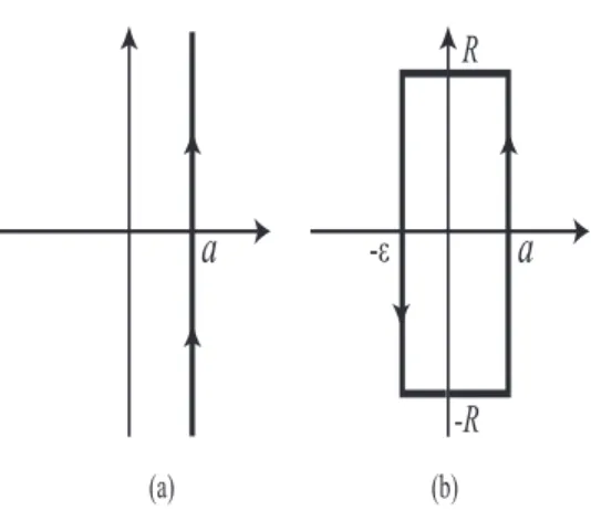
Figure 1: Deformation of the integral path for the Laplace inversion formula.

4 Asymptotic stability of the incoherent state

We now return to the problem of stability of the incoherent state. Recall that in the Fourier space the incoherent state corresponds to the trivial solution Z = (z

1

, z

2

, · · · ) = 0. The linearization about Z = 0 shows that it is a neutrally stable equilibrium of (2.8), (2.9) for 0 ≤ K < K

_c⁺

. There are no eigenvalues of T for these values of K and the continuous spectrum fills out the imaginary axis. Nonetheless, we show that the incoherent state is asymptotically stable with respect to the weak dual topology.

Theorem 4.1. For K ∈ [0, K

_c⁺

) the trivial solution of (2.8), (2.9) is an asymptotically stable equilibrium for initial data from X ⊂ X

⁰

with respect to the weak dual topology on X

⁰

.

Remark 4.2. The stability with respect to the weak dual topology is weaker than that with respect to the topology of the Hilbert space H. Still it is a natural topology for the problem at hand. In particular, Theorem 4.1 implies that the order parameter evaluated on the trajectories of the linearized problem tends to 0 as t → ∞.

Proof. Integrating (2.9) subject to z

_j

(0, ·) ∈ X, we have

z

j

(t, ·) = e

^ijωt

z

j

(0, ·), j ≥ 2.

By the Riemann-Lebesgue lemma, hz

_j

(t, ·), ψ(·)i =

Z

I

Z

R

e

^ijωt

z

j

(0, ω, x)ψ(ω, x)dωdx → 0, as t → ∞, ∀ψ ∈ X. (4.1) We now turn to (2.8). Consider the semigroup generated by the operator T on H given by the Laplace inversion formula

e

^tT

= lim

b→∞

1 2πi

Z

a+ib a−ib

e

^λt

(λ − T)

⁻¹

dλ, t > 0, (4.2)

where a > 0 is arbitrary. Thus, the (continuous) spectrum of T lies to the left of the integration path along

For arbitrary φ, ψ ∈ H, we have e

^tT

φ, ψ

H

= lim

b→∞

1 2πi

Z

a+ib a−ib

e

^λt

(λ − T)

⁻¹

φ, ψ

H

dλ. (4.3)

For φ, ψ ∈ X, (λ − T)

⁻¹

φ, ψ

H

is an analytic function in the right half–plane, which can be extended to the entire complex plane as a meromorphic function h R (λ)φ, ψi. Thus,

he

^tT

φ, ψi = lim

b→∞

1 2πi

Z

a+ib a−ib

e

^λt

h R(λ)φ, ψidλ ∀φ, ψ ∈ X. (4.4)

Let K ∈ [0, K

_c⁺

) be fixed. Next we claim that one can choose ε = ε(K) > 0 such that there are no generalized eigenvalues of T on or inside the contour

C

_ε,R

: a − iR → a + iR → −ε + iR → −ε − iR → a − iR (Fig. 1b)

for every R > 0. To construct C

_ε,R

with the desired property, we first fix δ > 0. Then we recall that generalized eigenvalues of T satisfy (3.12). From (3.13), under our assumptions on g, there exists R

0

= R

0

(δ) such that there are no roots of (3.12) in the region

D

⁺_R

0,δ

= {z ∈ C : |z| ≥ R

₀

& − δ < Re(z) ≤ a},

because (3.12) can be reduced to 2/(Kµ) = O(1/|λ|) in D

_R,δ⁺

for R 1. On the other hand, D(λ) is holomorphic. Thus, the set of roots of (3.12) (i.e., the set of generalized eigenvalues) does not have accumulation points in

D

⁻_R

0,δ

= {z ∈ C : |z| ≤ R

₀

& − δ < Re(z) ≤ a}.

Thus, we can choose ε > 0 such that there are no generalized eigenvalues in D

_R⁺

0,ε

∪ D

⁻_R

0,ε

. This completes the construction of C

ε,R

.

By the Cauchy Integral theorem, I

Cε,R

e

^λt

h R (λ)φ, ψidλ = 0 ∀φ, ψ ∈ X, (4.5) for any R > 0, and

Z

a+iR a−iR

e

^λt

h R (λ)φ, ψidλ =

Z

−ε+iR

−ε−iR

−

Z

−ε+iR a+iR

− Z

a−iR

−ε−iR

e

^λt

h R (λ)φ, ψidλ. (4.6)

Below, we show that the last two integrals on the right–hand side of (4.6) tend to 0 as R → ∞. Sending R → ∞ in (4.6) and using (4.4), we arrive at

he

^tT

φ, ψi = lim

R→∞

1 2πi

Z

−ε+iR

−ε−iR

e

^λt

h R (λ)φ, ψidλ

= e

^−εt

2πi lim

R→∞

Z

R

−R

ie

^iλt

h R (iλ − ε)φ, ψidλ

= O(e

^−εt

), ∀φ, ψ ∈ X

(4.7)

as t → ∞ because

Z

R

−R

ie

^iλt

h R (iλ − ε)φ, ψidλ

= O(1).

It remains to prove the following lemma.

Lemma 4.3. For K ∈ [0, K

_c⁺

),

R→∞

lim

Z

−ε+iR a+iR

e

^λt

h R (λ)φ, ψidλ = lim

R→∞

Z

a−iR

−ε−iR

e

^λt

h R (λ)φ, ψidλ = 0 ∀φ, ψ ∈ X. (4.8)

Proof. We show that the integral R

−ε+iR

a+iR

e

^λt

h R (λ)φ, ψidλ tends to zero as R → ∞. The second integral R

a−iR

−ε−iR

e

^λt

h R (λ)φ, ψidλ can be treated in the same way. Further, we decompose the integral into two integrals as

Z

−ε+iR a+iR

e

^λt

h R (λ)φ, ψidλ = Z

iR

a+iR

e

^λt

h R (λ)φ, ψidλ +

Z

−ε+iR iR

e

^λt

h R (λ)φ, ψidλ. (4.9) We show that the first integral on the right hand side tends to zero as R → ∞. For Re(λ) > 0, we have

h R (λ)φ, ψi = hA(λ)φ, ψi + K

2 hA(λ)W

I − K

2 D(λ)W

−1

D(λ)φ, ψi,

see (3.20). For the first term, we have Z

iR

a+iR

e

^λt

hA(λ)φ, ψidλ

= e

^iRt

Z

₀

a

e

^λt

Z

I

Z

R

1

λ + i(R − ω) φ(ω, x)ψ(ω, x)g(ω)dωdxdλ.

Since the integral above is finite, for any ε

₀

> 0, there exists L > 0 such that

Z

0 a

e

^λt

Z

I

Z

|ω|>L

1

λ + i(R − ω) φ(ω, x)ψ(ω, x)g(ω)dωdxdλ

< ε

0

On the other hand, the integrand

e

^λt

1

λ + i(R − ω) φ(ω, x)ψ(ω, x)g(ω) → 0,

as R → ∞ uniformly in x ∈ I, ω ∈ (−L, L) and λ ∈ (0, a). This implies that the integral Z

iR

e

^λt

hA(λ)φ, ψidλ → 0, as R → ∞.

Next, define a new function φ e

_λ

by φ e

λ

= W

I − K

2 D(λ)W

−1

D(λ)φ.

For 0 < K < K

_c⁺

, the operator T has no generalized eigenvalues in the right half plane and on the imaginary axis. This and (2.14) shows that I −

^K₂

D(λ)W

−1

is bounded uniformly in λ such that Re(λ) ≥ 0. Hence, φ e

_λ

is in X for any λ. Then the integral R

iR

a+iR

e

^λt

hA(λ) φ e

_λ

, ψidλ tends to zero by the same estimate as above.

This proves that R

iR

a+iR

e

^λt

h R (λ)φ, ψidλ decays to zero as R → ∞ . The second integral in (4.9) is estimated in a similar manner. This completes the proof of Lemma 4.3.

5 Bifurcation with a one-dimensional null space

In the previous section, we proved asymptotic stability of the equilibrium at the origin of the linearized system (2.8), (2.9) for K ∈ [0, K

_c⁺

). On the other hand, for K > K

_c⁺

there is a positive eigenvalue in spectrum of the linearized problem (cf. [3]). This signals a bifurcation at K

_c⁺

. This bifurcation is analyzed in this present section. As in the classical KM, the loss of stability of the incoherent state at K

_c⁺

and the development of partial synchronization for K > K

_c⁺

is best seen in terms of the order parameter.

Throughout this section, we assume that the largest positive eigenvalue µ

max

of W with the eigen- function w

_max

is simple. Furthermore, we assume that at K

_c⁺

there is a (one-dimensional) smooth center manifold of the equilibrium at the origin of (2.6), (2.7)

³

. Under these assumptions, below we show that the order parameter undergoes a supercritical pitchfork bifurcation at K

_c⁺

. The stable branch of equilibria bifurcating from 0 is given by

h

∞

(K) = g(0)

²

π

^3/2

p −g

⁰⁰

(0) µ

^3/2_max

s 1 C(x)

p K − K

c⁺

+ o( p

K − K

c⁺

), K > K

_c⁺

, (5.1) where

C(x) :=

Π ˜

_µmax

(|w

_max

|

²

w

_max

)

|w

_max

|

²

w

max

. (5.2)

Formula (5.1) generalizes the classical Kuramoto’s formula describing the pitchfork bifurcation in the all- to-all coupled model to the KM on graphs. The network structure enters into the description of the pitchfork bifurcation through the largest eigenvalue µ

max

and the corresponding eigenspace.

3The proof of existence of the center manifold is a technical problem and is beyond the scope of this paper (see [1] for the proof of existence of the center manifold in the original KM).

5.1 Preparation

Throughout this section, we assume that µ

max

is a simple eigenvalue of W. Let K = K

_c⁺

+ with 0 < 1 and rewrite (2.6),(2.7) as follows

∂

∂t z

₁

= T

₀

z

₁

+

2 Pz

₁

− K

2 Pz

₁

z

₂

, (5.3)

∂

∂t z

j

= ijωz

j

+ jK

2 Pz

1

z

j−1

− Pz

1

z

j+1

, j = 2, 3, . . . , (5.4) where T

₀

is T estimated at K = K

_c

and T = T

₀

+ P/2.

For small > 0, the equilibrium of (5.3), (5.4) at the origin has a 1D unstable manifold. We reduce the dynamics on the 1D unstable manifold, which we approximate by the center manifold of the origin for K = K

_c⁺

, i.e., for = 0. For the latter, we assume z

_k

= h

_k

(z

₁

), k = 2, 3, . . . , on the center manifold, where h

k

are smooth functions such that h

k

(0) = h

⁰_k

(0) = 0.

Let Π

0

be the projection to the eigenspace of λ = 0 spanned by v

_c⁺

(cf. Section 3.4). To track the evolution on the slow manifold we adopt the following Ansatz:

z

1

= Π

0

z

1

+ (I −Π

₀

)z

1

= αc(t)v

_c⁺

+ O(α

²

), (5.5) z

k

= h

k

(z

1

) = O(α

²

), k = 2, 3, . . . , (5.6)

= α

²

, (5.7)

where α > 0 is a small parameter, c(t) is the coordinate along the center manifold, and v

⁺_c

is the generalized eigenfunction of T

0

corresponding to the zero eigenvalue (cf. (3.15)). The Ansatz (5.5)-(5.7) follows right away once existence of the center manifold is shown.

We will start by deriving several auxiliary facts that follow from the Ansatz (5.5)-(5.7). First, using (5.5)-(5.7) and Theorem 3.4, from (5.3), we have

˙

z

₁

= T

₀

z

₁

+ O(α

²

) = T

^×₀

(αc(t)v

_c⁺

) + O(α

²

) = O(α

²

). (5.8) Next, we estimate the order parameter.

Lemma 5.1.

h(t, x) = αc(t)w

_max

(x) + O(α

²

). (5.9) Proof.

h = Pz

1

= P αc(t)v

_c⁺

+ O(α

²

)

= αc(t) K

_c⁺

2 lim

λ→0+

Z

R

Z

I

W (x, y)w

max

(y)g(ω)

λ − iω dydω + O(α

²

). (5.10)

Applying the Fubini theorem, (3.12) and (2.15), we have h = αc(t) K

_c⁺

2 (Ww

max

)D(0+) + O(α

²

)

= αc(t) K

_c⁺

µ

_max

2 D(0+)w

_max

+ O(α

²

)

= αc(t)w

max

+ O(α

²

).

(5.11)

Lemma 5.2.

z

₂

=

αc(t)K

_c⁺

2

2 λ→0+

lim*

w

²_max

(λ − iω)

²

+ O(α

³

). (5.12)

Proof. Using (5.5)-(5.7) and (5.8), we obtain

˙

z

₂

= h

⁰₂

(z

₁

) ˙ z

₁

= O(α

³

),

(Pz

1

)z

3

= O(α

³

). (5.13)

By plugging (5.13) into (5.4) for j = 2, we obtain

0 = 2iωz

₂

+ K(Pz

₁

)z

₁

+ O(α

³

). (5.14) Next we plug in the expressions for z

₁

, Pz

₁

, and z

₂

(see (5.5), (5.9), (5.12)) into (5.14) to verify that they satisfy this equation up to O(α

³

) terms. Specifically, we have

2iωz

2

+ K(Pz

1

)z

1

= 2iω

αc(t)K

_c⁺

2

2 λ→0+

lim*

w

²_max

(λ − iω)

²

+ K αc(t)w

max

+ O(α

²

)

αc(t)v

⁺_c

+ O(α

²

)

+ O(α

³

)

= −α

²

c(t)

²

(K

_c⁺

)

²

2 lim*

λ→0+

(λ − iω) − λ (λ − iω)

²

w

²_max

+ K

_c⁺

α

²

c(t)

²

w

max

K

_c⁺

2 lim*

λ→0+

w

max

λ − iω + O(α

³

)

= −α

²

c(t)

²

(K

_c⁺

)

²

2 lim*

λ→0+

w

_max²

λ − iω + α

²

c(t)

²

(K

_c⁺

)

²

2 lim*

λ→0+

w

_max²

λ − iω + O(α

³

)

= O(α

³

).

5.2 The slow manifold reduction

Projecting both sides of (5.3) onto the center subspace, we have Π

0

z ˙

1

= Π

0

T

0

z

1

+

2 Π

0

h − K

2 Π

0

(hz

2

). (5.15)

Using (5.5), we have

Π

₀

z ˙

₁

= α c(t)v ˙

_c⁺

,

Π

0

T

0

z

1

= T

^×₀

Π

0

z

1

= αc(t)T

^×₀

v

_c⁺

= 0. (5.16) Further,

Π

₀

h = g

₁

lim*

λ→0+

(λ − iω)

⁻¹

Π ˜

_µmax

D(λ)h. (5.17) To evaluate (5.17), we take the following steps

λ→0+

lim* D(λ)h = lim*

λ→0+

Z

R

αc(t)w

_max

λ − iω g(ω)dω + O(α

²

)

= αc(t)w

max

D (0+) + O(α

²

)

= 2αc(t)w

_max

K

_c⁺

µ

_max

+ O(α

²

) and

λ→0+

lim

Π ˜

µmax

D(λ)h = 2αc(t)w

max

K

c⁺

µ

_max

+ O(α

²

).

Finally,

Π

₀

h = 2αc(t) K

c⁺

µ

max

g

₁

lim*

λ→0+

w

_max

λ − iω + O(α

²

)

= αc(t) µ

max

g

1

2 K

c⁺

2

v

⁺_c

+ O(α

²

).

(5.18)

Similarly, to evaluate

Π

0

(hz

2

) = g

1

lim*

λ→0+

(λ − iω)

⁻¹

Π ˜

µmax

D(λ)(hz

2

), (5.19) we first compute

λ→0+

lim* D(λ)(hz

2

) = α

³

|c(t)|

²

c(t) K

_c⁺

2

2

|w

_max

|

²

w

max

lim

λ→0+

Z

R

g(ω)dω

(λ − iω)

³

+ O(α

⁴

)

= −α

³

|c(t)|

²

c(t)g

₂

K

_c⁺

2

2

|w

_max

|

²

w

_max

+ O(α

⁴

),

(5.20)

where

g

₂

= πg

⁰⁰

(0)

2 . (5.21)

By plugging (5.20) into (5.19), we obtain

−α

³

|c(t)|

²

K

_c⁺

Π ˜

_µmax

(|w

_max

|

²

w

_max

)

_{+ 4}