入力関数に肺微分曲線を用いた

I.     は じ め に

N-isopropyl-4-¹²³I-iodoamphetamine (以下 ¹²³I-

IMP) の局所脳血流量算出方法は，Kuhl ら¹⁾ が考

案したマイクロスフェアモデルに基づいた持続動 脈採血法²⁾ や Iida ら³⁾ が開発した一回動脈採血法 (以下 ARG 法) が使用されている．これらは，入 力関数を求める方法としては信頼性や再現性に優 れているが侵襲性において難点がある．近年，無 採血の非侵襲的な脳血流定量法として，宮崎らの

FU 変法⁴⁾ や米倉らの非侵襲的マイクロスフェア

法⁵⁾ (以下 NIMS 法) が開発され臨床に使用されて

いる．しかし，手技の繁雑性から一般に普及され るまでに至っておらず，より簡便な方法の開発が 望まれている．

99mTc-製剤では，Patlak plot 法を応用した無採

《原  著》

入力関数に肺微分曲線を用いた

I-IMP-Patlak plot 法の検討

――NIMS 法による脳血流量との比較――

伊勢谷 修* 三原 常径* 鈴木 健之** 宮前 達也**

松田 博史***

要旨 ¹²³I-IMPを用いた非侵襲的でより簡便な脳血流定量法として Patlak plot 法が臨床応用可能か検

討した．投与された ¹²³I-IMP は，肺にすべて一時的に集積した後，肺動脈血流により洗い出され，中 心循環系に拡散するものと仮定し，脳から肺野全体をカメラ視野内に入れ，ダイナミックデータを収集 した．肺のクリアランス曲線 L(t) を微分した後，CO (心拍出量) で除してプラス成分に変換し，単位時 間当たりに動脈血中に拡散する ¹²³I-IMPトレーサ濃度を求め，これを動脈血時間放射能曲線 A(t) とし た．A(t) と全脳時間放射能曲線 B(t) との間で Patlak plot 解析を行い K1 (全脳血流量 tCBF ml/min) と Vn

(非特異的初期分布容積 ml) を求めた．また，肺に残存するトレーサ量 [Lpeak−L(T)] から，時間 (T) ま

で中心循環系に拡散したトレーサの総量が求まり，これを経時的に行うことで集積曲線が得られる．こ の集積曲線を微分すると，単位時間当たりに中心循環系に拡散するトレーサ量を推定することができ る．これを入力関数指標 I(t) として，Patlak plot 解析を行い一方性流入指標 ki を求め，100 を乗じて脳 血流指標 (IMP-BPI) とした．脳血管障害および神経疾患を有する患者 16 症例を対象とし，同時に施行 した非侵襲的マイクロスフェア法で得られた平均脳血流値 (mCBF) に対して，K1 および IMP-BPI の相 関を求め両者を比較検討した．K1 と mCBF の相関は，r＝0.759 (y＝0.032x＋20.1), ki から求めた IMP- BPI では，r＝0.833 (y＝2.73x＋0.10) となり，両者とも強い相関関係が得られたが IMP-BPI の方が良い 結果となった．以上の結果から，入力側と流入側を同時に測定する ¹²³I-IMP-Patlak plot 法は，簡易的な 入力関数を用いても，非侵襲的な方法として臨床応用が可能であると判断した．

(核医学 40: 163–174, 2003)

*埼玉医科大学附属病院核医学診療部

**埼玉医科大学放射線科

***国立精神・神経センター武蔵病院放射線診療部 受付：14 年 1 月 25 日

最終稿受付：15 年 4 月 8 日

別刷請求先：埼玉県入間郡毛呂山町毛呂本郷 38 (0 350–0495)       埼玉医科大学附属病院核医学診療部

伊勢谷   修

血で非侵襲的な簡便法が Matsuda ら⁶⁾ によって開 発され (以下 Patlak plot-松田法) 広く臨床に使用 されている．この方法は，BPI (脳血流指標) を求

め，¹³³Xe の局所脳血流量の回帰式より平均脳血

流量を換算している．

今回，われわれは，¹²³I-IMP を用いた定量法の 定量手技における一層の簡易化を目的として，投 与された ¹²³I-IMP が肺にすべて一時的に集積した 後，肺動脈血流によって洗い出され中心循環系に 拡散し，ある一定の割合で脳に摂取されるトレー サ動態モデルを想定した．

データ収集には，大視野ガンマカメラ装置を用 い，脳から肺野全体をカメラ視野内に入れダイナ ミックデータ収集 (1 フレーム／秒) を行った．肺 のクリアランス曲線 L(t) を微分した後，CO (心拍 出量) で除してプラス成分に変換し，単位時間当 たりに動脈血中に拡散する ¹²³I-IMP トレーサ濃度 を求め，これを動脈血時間放射能曲線 A(t) とし た⁵⁾．A(t) と全脳時間放射能曲線 B(t) との間で Patlak plot 解析を行い K1 (全脳血流量 tCBF ml/

min) と Vn (非特異的初期分布容積 ml) を求めた．

一方，肺に残存するトレーサ量 [Lpeak−L(T)] か ら，時間 (T) までに中心循環系に拡散したトレー サの総量が求まり⁸⁾，これを経時的に行うことで 集積曲線 W(t) が得られる．この W(t) を微分する と単位時間当たりに中心循環系に拡散するトレー サ量から CO 成分を算出しない近似的な入力関数 を推定することができる．これを入力関数指標 I(t) として，Patlak plot 解析を行い一方性流入指標 k_i を求め，100 を乗じて脳血流指標 (IMP-BPI) と した．

局所脳血流量 (ml/g/min) を算出するには，K1 で は全脳の重量が必要である．また，一方性流入指 標 ki は，K1 の相対値であり，両者とも Patlak plot- 松田法と同様に局所脳血流量との換算が必要であ る．そこで，NIMS 法を同時に施行し，得られた 平均脳血流量 (以下 NIMS-mCBF) と K1 および ki

から求めた IMP-BPI との相関および回帰式を求 め，より簡便な方法が臨床応用可能かを比較検討 した．

II.     対象および方法

1. 対象症例

脳梗塞 10 例，モヤモヤ病 1 例，脳出血 1 例，

アルツハイマー病 4 例の合計 16 例であり，男性 13 例，女性 3 例で年齢は 14〜72 歳，平均は 58.5

±19.6 歳で，いずれも心肺疾患を認めない症例で ある．

2. データ収集

167 MBq の ¹²³I-IMP を右側肘静脈に 21 G 翼状 針，1.9 ml 容量の延長チューブ，三方活栓で確保 し，生食 20 ml を用いてボーラス注入した．

中エネルギー用コリメータ (以下 MEGAP コリ メータ) を装着した Picker 社製大視野 3 検出器カ メラ装置 PRISM-IRIX (有効視野 533 mm×394 mm) をコの字型にセットして，長軸方向に脳から 肺野全体がカメラ視野に入るようセッティングし た．ダイナミックデータは，64×64 マトリック ス，1 フレーム／秒で 0〜600 秒間を収集し，得 られたデータに 3 フレームの画像加算処理 (3 秒 加算) を行い 200 フレームに圧縮した．また，

NIMS 法のデータ収集は，米倉らの報告に準じて 行った．

3. 方  法

1) 脳および肺の関心領域 (regions of interest   以下 ROI) の設定 (Fig. 1)

肺クリアランス曲線のピークカウントおよび ピーク位置を正確に求めることを目的として，鎖 骨下静脈，上大静脈，右心および肺動脈が描画で きるよう画像加算し，鎖骨下静脈から肺動脈まで ROI-1 (Fig. 1-a) を設定した．その後，肺の集積画 像 (90〜150 秒間加算) を表示させ，ROI-1 が含ま れないよう左右の肺にそれぞれ ROI-2, 3 (Fig. 1- b) (画像表示の閾値は最高カウントの 20%) を設定 した．脳 ROI は，肺の最高カウントの影響を受 け，ROI の作成が困難である．そのため，画像調 整 (閾値は 0% で upper level 調整) を行い全脳に 楕円形 ROI-4 (Fig. 1-c) を設定した．なお，脳の 画像は，240〜300 秒間を加算して表示した．

入力関数に肺微分曲線を用いた I-IMP-Patlak plot 法の検討 165

Fig. 1

Setting of the ROIs (region of interest). a: Setting of the ROI for the subclavian vein, superior vena cava, right heart region and pulmonary artery. b: Setting of ROI-2 and ROI-3 for the right and left lung, respectively, without inclusion of ROI-1. c:

Setting of elliptic ROI-4 on the whole brain image.

Fig. 2

Pulmonary clearance curve and the brain time-activity curve. a: Clearance curve for the Rt. Lung and the Lt.

Lung, and the time-activity curve (TAC) of the whole brain. b: Pulmo- nary clearance curve after the addition of the Rt. and Lt. Lung counts.

Fig. 3

Differential curve for pulmonary clearance and input function A(t). a:

Pulmonary differential curve ∆L(t).

b: ∆L is multiplied by a negative value and converted to a positive component to be used as an arterial time-activity A(t), B(t)＝whole brain TAC.

Fig. 4

Simplified Compartmentation and calculation of the input function index. a: Simplified Computation model. b: W(t) represents the ac- cumulation curve obtained from sequention calculation of peak Lpeak

−L(t). The input function index I(t) is determined by differentiating the curve. [W(t)＝∫I(t)]

Fig. 5

Normalization of ∫I(t)dt curve and B(t). a: ∫I(t)dt curve obtained by integrating input function index I(t) and whole brain TAC B(t). b: Both curver were normalized by a 5- minute counts.

Fig. 6

Changes in the mean values of K1

and IMP-BPI over time and their standard deviation. Mean values dropped in both cases over time.

Fig. 7

Changes in the mean values of Vn

and Vi over time and their standard deviation. Negative values were obtained in both cases at certain times．

Fig. 9

Representative examples of nor- malization of ∫I(t)dt curve and B(t).

a: Case No. 5, b: No. 12. c: A case excluded because respiratory vari- ations were too great and normali- zation was inappropriate.

Fig. 7 Fig. 6

Fig. 9

入力関数に肺微分曲線を用いた I-IMP-Patlak plot 法の検討 167

Fig. 8

Chart of duration of analysis and plot. a: Data between A(t) and B(t), b: Data between I(t) and B(t) take the form of approximately a straight line along the plot dots.

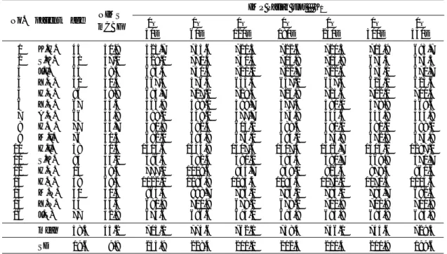
Table 1 NIMS-mCBF and K1 in the examined subjects

NIMS IMP Patlak plot K1

No. patient age

mCBF 0– 0– 0– 0– 0– 0– 0–

30s 60s 120s 180s 240s 300s 540s

1 K.H. 45 50.9 525.7 735.6 721.3 722.6 720.3 715.9 693.7

2 S.K. 51 37.0 328.1 770.4 740.4 704.8 704.8 674.3 674.3

3 J.I. 63 48.4 685.5 730.6 721.0 722.7 722.6 674.0 670.7

4 Y.T. 51 40.4 667.4 576.5 635.5 647.0 647.3 625.1 623.6

5 H.T. 86 49.8 693.7 727.0 728.3 726.8 725.6 712.0 700.5

6 Y.T. 67 35.3 556.9 589.1 599.7 577.5 580.0 578.8 569.6

7 A.T. 66 34.8 498.0 559.0 577.7 575.9 544.6 543.9 543.9

8 H.O. 77 35.7 580.9 592.5 605.2 589.3 591.0 591.0 599.0

9 M.I. 76 40.5 682.0 693.9 676.0 684.0 673.9 672.8 673.9

10 H.I. 38 51.4 1305.6 1333.9 1307.6 1307.3 1306.7 1305.1 1287.1

11 S.K. 84 43.1 596.4 582.5 581.2 584.5 581.7 569.9 571.7

12 H.T. 14 59.4 777.1 1019.6 945.7 938.1 926.4 878.5 861.6

13 H.S. 38 68.3 1122.1 1196.9 1184.4 1184.6 1172.2 1171.6 1105.6

14 M.N. 50 50.4 863.5 898.7 796.0 796.0 795.0 794.7 692.6

15 Y.N. 53 45.4 691.9 700.9 679.2 679.2 711.8 711.8 710.9

16 J.T. 77 32.8 674.6 686.6 694.0 693.8 693.8 693.8 693.8

mean 58.5 45.2 703.1 774.6 762.1 758.4 756.1 744.6 729.5

SD 19.6 9.8 235.9 228.4 211.1 212.3 211.4 211.9 199.6

NIMS-mCBF: Noninvasive Microsphere Method-mean Cerebral Blood Flow (ml/100 g/min) K1: total cerebral blood flow (ml/min), s: sec

2) 肺のクリアランス曲線と全脳時間放射能曲   線 B(t) の作成 (Fig. 2)

肺のクリアランス曲線は，肺 ROI-2, 3 の各々の クリアランス曲線 (Fig. 2-a) を作成し，両曲線を 加算 (Fig. 2-b) した．全脳時間放射能曲線 B(t) (Fig.

2-a) は，全脳 ROI-4 より求めた．いずれも，1〜

200 フレーム (600 秒間) まで行い，得られた両曲 線に 3 点タイムスムージング処理を加え Patlak

plot 解析に必要なデータを作成した．

3) 動脈血時間放射能曲線 A(t) と入力関数指標    

   I(t) の算出

肺のクリアランス曲線 L(t) を微分し，NIMS 法で 求めた心拍出量 CO で除してマイナス (−1) を乗じ て正の成分に変換させ，単位時間当たりに動脈血 中に流入する ¹²³I-IMP のトレーサ量を求め，これ を動脈血時間放射能曲線 A(t) とした (Fig. 3-a, b)．

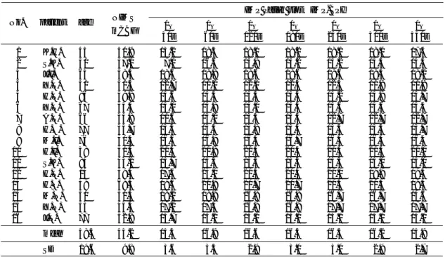
Table 2 Vn in the examined subjects IMP Patlak plot Vn

No. patient age 0– 0– 0– 0– 0– 0– 0–

30s 60s 120s 180s 240s 300s 540s

1 K.H. 45 2775.1 1505.5 1981.4 1374.3 834.7 684.4 3070.3

2 S.K. 51 5598.2 2482.6 2193.5 2933.1 2382.3 4320.7 1485.1

3 J.I. 63 793.9 −35.3 −619.7 −1235.0 −1806.6 3176.2 1861.0

4 Y.T. 51 52.4 959.7 −485.3 −1017.6 −1388.6 1615.3 457.4

5 H.T. 86 −16.7 −688.2 −1129.2 −1071.0 −920.2 1599.3 3143.9

6 Y.T. 67 267.8 −39.3 −883.0 559.9 178.5 −763.3 3027.4

7 A.T. 66 1169.5 793.6 −679.4 −778.9 2357.8 2992.7 2044.1

8 H.O. 77 397.2 327.3 −12.6 1229.3 1927.7 1963.7 591.5

9 M.I. 76 362.5 215.0 262.6 −444.3 1319.1 737.0 1981.3

10 H.I. 38 1133.5 253.6 102.5 −3314.4 −5306.2 −6528.8 −8421.4

11 S.K. 84 172.1 19.3 −199.6 −520.5 −658.7 566.9 228.0

12 H.T. 14 3359.3 814.5 289.6 −1248.6 −1967.5 797.2 1669.6

13 H.S. 38 1984.6 1520.5 −18.2 −1514.4 −3637.4 −5041.6 172.1

14 M.N. 50 1201.8 94.3 −4922.7 −5131.2 −6378.2 −6914.9 274.8

15 Y.N. 53 172.4 −35.4 1366.3 1389.5 −3090.7 −2682.2 −1680.7

16 J.T. 77 313.0 99.7 −585.1 −9124.1 −7727.9 −6951.2 −4359.3

mean 58.5 1233.5 518.0 −208.7 −1119.6 −1492.6 −651.8 346.6

SD 19.6 1531.2 790.7 1587.9 2868.1 3092.6 3775.9 3017.5

Vn: initial distribution volume (ml)

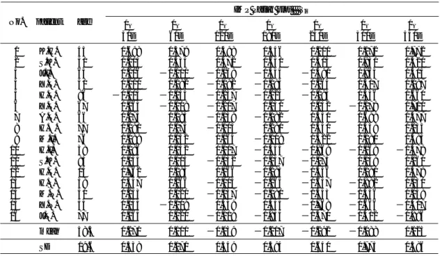
Table 3 NIMS-mCBF and BPI in the examined subjects

NIMS IMP Patlak plot IMP-BPI

No. patient age

mCBF 0– 0– 0– 0– 0– 0– 0–

30s 60s 120s 180s 240s 300s 540s

1 K.H. 45 50.9 13.2 18.5 18.1 18.2 18.1 18.0 17.4

2 S.K. 51 37.0 7.1 16.6 15.9 15.2 15.2 14.5 14.5

3 J.I. 63 48.4 18.6 19.8 19.6 19.6 19.6 18.3 18.2

4 Y.T. 51 40.4 12.7 11.0 12.1 12.3 12.3 11.9 11.9

5 H.T. 86 49.8 14.6 15.3 15.3 15.3 15.2 14.9 14.7

6 Y.T. 67 35.3 13.1 13.8 14.1 13.5 13.6 13.6 13.4

7 A.T. 66 34.8 11.6 13.0 13.5 13.4 12.7 12.7 12.7

8 H.O. 77 35.7 13.3 13.5 13.8 13.4 13.5 13.5 13.7

9 M.I. 76 40.5 16.6 16.9 16.5 16.7 16.4 16.4 16.4

10 H.I. 38 51.4 21.4 21.8 21.4 21.4 21.4 21.4 21.1

11 S.K. 84 43.1 15.7 15.3 15.3 15.3 15.3 15.0 15.0

12 H.T. 14 59.4 17.6 23.1 21.5 21.3 21.0 19.9 19.5

13 H.S. 38 68.3 19.6 20.9 20.7 20.7 20.5 20.5 19.3

14 M.N. 50 50.4 18.2 18.9 16.8 16.8 16.7 16.7 14.6

15 Y.N. 53 45.4 17.2 17.4 16.9 16.9 17.7 17.7 17.7

16 J.T. 77 32.8 13.7 14.0 14.1 14.1 14.1 14.1 14.1

mean 58.5 45.2 15.3 16.9 16.6 16.5 16.5 16.2 15.9

SD 19.6 9.8 3.6 3.5 2.9 3.0 3.0 2.9 2.7

IMP-BPI: ¹²³I-IMP-brain perfusion index (ki×100)

入力関数に肺微分曲線を用いた I-IMP-Patlak plot 法の検討 169

また，肺に残存するトレーサ量 [Lpeak−L(T)] か ら，時間 (T) までに中心循環系に拡散したトレー サの総量が求まり，これを継時的に行い集積曲線 W(t) を求めた．この W(t) を微分することで，単 位時間当たりに中心循環系に拡散するトレーサ量 を推定し，これを入力関数指標 I(t) とした (Fig.

4-b)．

4)     Patlak plot 解析の開始点と解析時間の設定 A(t) と I(t) は，肺クリアランス曲線 L(t) のピー ク点で 0 の値となる．この点を解析の開始点 (0 秒 とする) として，0〜30 秒間，0〜60 秒間，0〜120 秒間，0〜180 秒間，0〜240 秒間，0〜300 秒間，

0〜540 秒間の 7 点の解析時間を設定した．

A(t) と全脳時間放射能曲線 B(t) の間で，下記の (3) 式によりグラフプロット解析を行い直線近似 することにより，それぞれの全脳血流量 K1 (tCBF ml/min) と非特異的初期分布容積 V_n (ml) を求め た．しかし，入力関数 A(t) と I(t) は，測定時間が 90 秒以降になると，データの変動により負の値 が生じる．そのため，これらの値を削除して解析

を行った．また，I(t) では，下記の (5) 式を用い て A(t) の方法と同様に解析を行い，一方性流入指

標 ki を求め 100 を乗じて，IMP-BPI とした．ま

た，Vi を非特異的初期分布指標と定義した．

5) 理論式

動脈血時間放射能曲線 A(t) の算出式

A(t)＝−∆L(t)/CO (1)

この動脈血時間放射能曲線 A(t) と B(t) との間で，

Patlak plot 解析を行い K1 と Vn を求めた．

B(t)＝K1・ A(t)dt＋VnA(t) (2) B(t)＝K1・ A(t)dt

＋Vn (3)

A(t) A(t)

(3) 式に (1) 式を代入すると

CO・ B(t)

＝K1・ ∆L(t)dt

＋Vn (4) −∆L(t) ∆L(t)

となる．

Table 4 Vi in the examined subjects IMP Patlak plot Vi

No. patient age 0– 0– 0– 0– 0– 0– 0–

30s 60s 120s 180s 240s 300s 540s

1 K.H. 45 0.698 0.379 0.498 0.346 0.210 0.172 0.772

2 S.K. 51 1.205 0.534 0.472 0.631 0.513 0.930 0.320

3 J.I. 63 0.216 −0.010 −0.168 −0.335 −0.491 0.863 0.505

4 Y.T. 51 0.010 0.182 −0.092 −0.193 −0.264 0.307 0.087

5 H.T. 86 −0.004 −0.144 −0.237 −0.225 −0.193 0.336 0.660

6 Y.T. 67 0.063 −0.009 −0.207 0.131 0.042 −0.179 0.710

7 A.T. 66 0.273 0.185 −0.159 −0.182 0.550 0.699 0.477

8 H.O. 77 0.091 0.075 −0.003 0.280 0.440 0.448 0.135

9 M.I. 76 0.088 0.052 0.064 −0.108 0.322 0.180 0.483

10 H.I. 38 0.186 0.042 0.017 −0.543 −0.869 −1.069 −1.379

11 S.K. 84 0.045 0.005 −0.052 −0.137 −0.173 0.149 0.060

12 H.T. 14 0.762 0.185 0.066 −0.283 −0.446 0.181 0.379

13 H.S. 38 0.347 0.266 −0.003 −0.265 −0.637 −0.882 0.030

14 M.N. 50 0.253 0.020 −1.037 −1.080 −1.343 −1.456 0.058

15 Y.N. 53 0.043 −0.009 0.339 0.345 −0.768 −0.666 −0.417

16 J.T. 77 0.064 0.020 −0.119 −1.854 −1.570 −1.412 −0.886

mean 58.5 0.271 0.111 −0.039 −0.217 −0.292 −0.088 0.125

SD 19.6 0.338 0.171 0.349 0.594 0.640 0.775 0.586

Vi: initial distribution index

∫

∫

∫

入力関数指標 I(t) からの算出式

(4) 式で，CO が患者間で群間差が少なくほぼ一 定な値であると仮定すると (5) 式が得られる．

入力関数指標 I(t) は，Lpeak−L(T) の集積曲線 W(t) を微分することにより求めた．この I(t) を入 力関数として B(t) との間で，Patlak plot 解析を行 い一方性流入指標 ki を求めた．

B(t)

＝ki

I(t)dt

＋Vi (5) I(t) I(t)

IMP-BPI＝100×ki (6)

ゆえに IMP-BPI は，全脳血流量 K1 の相対値であ るため，CO がある一定の範囲内で成立する解析 法である．

6) データの信頼性の検証 (Fig. 5)

Lpeak−L(T) の集積曲線 W(t) は，I(t) を積分し た  I(t)dt 曲線と表すことができる (Fig. 5-a)．

I(t)dt 曲線と全脳時間放射能曲線 B(t) とをグラ フ上 (5 分のカウント数) (Fig. 5-b) で正規化し，

本法のデータの信頼性を確認した．なお，正規化 によって重ね合わせが不十分であった症例は，今 回のデータから除外した．

7)     SPECT 収集および画像処理

SPECT 収集は，投与 20 分後から MEGAP コリ メータにて，128×128 マトリックス，拡大 1.60 倍，1 検出器につき120°，一方向 12.5 秒 (計 72 方向) の連続収集モードで 4 回転収集した (撮像 時間 20 分)．SPECT 像の再構成には，再構成フィ ルターとしてランプフィルター，後処理フィル ターとしてバターワースフィルターを用い，吸収 補正は行わなかった．

8)     NIMS 法の解析

NIMS 法の解析に必要な脳の 5 分値 (Cb 5 min) は，300 秒から 30 秒間を加算し求めた．また，

肺の洗い出し比は，300 秒から 30 秒間を加算し 平均カウントを求め，肺のピークカウントで除し 算出した．また，肺 ROI 作成は，90 秒から 60 秒 間を加算し画像表示 (100〜0% 表示) させ，Fig. 1- a, b に従って行った．

9)     NIMS 法との検討

K1 は，全脳の質量が加味されておらず，IMP-

BPI は，脳血流の指標値である．そのため，同時 に施行した NIMS 法より求めた mCBF との相関 および回帰式を各々の解析時間毎に求め比較検討 した．

III.     結  果

各症例の解析時間毎の K1, Vn および IMP-BPI，

Vi と NIMS-mCBF の結果と平均値を Table 1, 2, 3, 4 に示す．

K1の解析時間毎の平均は 703±236 ml/min〜

775±228 ml/min で，IMP-BPI の解析時間毎の平 均は 15.26±3.57〜16.87±3.47 で，ほぼ一定の値 となったが K1 および IMP-BPI の時間的推移 (Fig.

6-a, b) は，0〜60 秒間の解析をピークに緩やかに 減少し，0〜540 秒間で K1 は 5.8%, IMP-BPI は 5.7% 低下した．

Vn と Vi の平均値の時間的推移 (Fig. 7-a, b) は，

最大 1234±1531 ml，最小 −1493±3093 ml で，

Viは最大 0.27±0.34，最小 −0.29±0.59 となり 両者とも解析時間によっては，負の値となった．

また，グラフプロット図は，両者とも解析時間に 関係なくほぼ直線上に分布した．Fig. 7-a, b はそ の代表例である．

集積曲線

(

)

17 例中16 例で両曲線が一致した．その代表例 (Fig. 9-a, b) と呼吸変動で両曲線が一致せず除外し た症例を Fig. 9-c に示す．なお，両曲線の 5 分で のカウント比の平均は，6.41±1.04 であった．

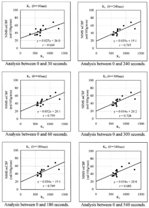
対象 16 例における K1と IMP-BPI と NIMS- mCBF との相関を Fig. 10 および Fig. 11 に示す．

K1 では，0〜30 秒間の解析で r＝0.660 となり，

それ以降では，r＝0.685〜0.759 の値が得られ た．回帰式は，0〜60 秒間 (r＝0.759) で y＝0.032x

＋20.1 となり，IMP-BPI は，0〜30 秒間の解析で r＝0.678 となり，それ以降では，r＝0.755〜0.833 の値が得られた．回帰式は，0〜180 秒間 (r＝

0.833) で y＝2.73x＋0.10 となった．

∫

∫

∫

∫

入力関数に肺微分曲線を用いた I-IMP-Patlak plot 法の検討 171

NIMS-mCBF の平均は 45.2±7.8 ml/100 g/min で 肺の洗い出し比の平均は 0.402±0.096， 心拍出量 (CO) の平均は 4569±674 ml/min であった．

IV.     考  察

123I-IMP は，一時的に肺に集積した後，動脈血

中に洗い出される特性を有している．Yonekura ら⁷⁾ は，ダイナミック SPECT とシンチレーショ ンカウンターを用いて，肺のクリアランス曲線の 半減期 (T1/2) と脳時間放射能曲線の 90% 到達時間

(T0.9) が相関することを報告している．また，米

倉ら⁸⁾ は，FU 法で肺のクリアランス曲線のピー ク点からある時間 (T) までの全身に拡散する ¹²³I- IMP の総量と脳の集積カウントから摂取比 (frac-

tional uptake, 以下 FU) を算出し，FU 値が肺の ピークカウントから 30 秒間は変動したがその後 は，ほぼ一定であると報告している．

入力関数指標 I(t) を積分して求めた I(t)dt 曲 線は，肺のピークからある時間 (T) までに中心 循環系に拡散したトレーサ量の総量であり，FU 法での Q-L(t) の曲線と同一の曲線となる．この

 I(t)dt 曲線と全脳時間放射能曲線 B(t) との正規

化で，両曲線が立ち上がり部分からほぼ一致した ことは，全脳時間放射能曲線 B(t) は，投与早期か ら肺のクリアランス曲線に依存していることを示 している．

Yokoi ら⁹⁾ は頻回な動脈採血とダイナミック

SPECT から 2 コンパートメントモデル Cb(t)＝

Fig. 10 Correlation between K1 of the analytic time and NIMS-mCBF. The coefficient of correlation is almost constant, regardless of the duration of measurement. K1 (0–60 sec) showed the strongest correlation (r＝0.759)．

Fig. 11 Correlation between IMP-BPI of the analytic time and NIMS-mCBF. As with K1, almost constant values were obtained regardless of the period of analysis. IMP-BPI (0–180 sec) showed the strongest correlation (r＝0.833)．

∫

∫

K Ca(s)ds−k2 Cb(s)ds 式から脳血流量 K1 (ml/

g/min) と脳からの洗い出し定数 k2 (min⁻¹) および 分配係数 λ を求めている．本法での IMP-BPI の 平均も 0〜60 秒間の値をピークに解析時間の終了 点を延長するにつれ緩やかに低下しており，脳か らの洗い出しの影響を受けているものと推測され る．

本来なら持続動脈採血法や ARG 法を比較対象 とすべきであるが，中野ら¹⁰⁾ は持続動脈採血法と FU 変法による CBF factor と比較検討し r＝0.962 ときわめて高い相関が得られたことを報告してい る．さらに，Kaminaga ら¹¹⁾ は，ARG 法と NIMS 法との検討を行い回帰式 y＝0.90x＋6.39 で，r＝

0.70 の相関があることを報告している．また，

宮崎らは，FU 法の改良法で ^99mTc-HM-PAO での Patlak plot-松田法と比較し，r＝0.833 の相関があ ることを報告している．これらのことから NIMS 法は，比較対象として妥当であると考えている．

本法は，急速注入により ¹²³I-IMP をできるだけ 瞬時に肺に集積させることが必要である．また，

123I-IMP から放出する 529 keV の γ-ray の影響を 充分に配慮したコリメータの選択が重要である．

千田ら¹²⁾ が提唱した数え落とし補正法での検討で

は，低エネルギー用高分解能 (以下 LEHR) コリ メータは y＝−0.0129x＋1.000， MEGAP コリ メータでは y＝−0.0047x＋1.00 の補正式が得られ た ． こ の 結 果 か ら ，L E H R コ リ メ ー タ は ， MEGAP コリメータに比べ数え落とし率が高く，

入力関数 [A(t) と I(t)] を正確に求めることができ ない．また，全脳時間放射能曲線 B(t) は，急速注 入時の高カウント領域 (鎖骨下静脈など) からの隔 壁通過線と散乱線の影響を受け，曲線の立ち上が り部分のデータを正確に測定することができな い．そのため，これらの影響をできるだけ排除す る目的で，中エネルギー用コリメータを使用し データ収集を行った．しかしながら，NIMS 法で の投与前シリンジカウント測定では，1.1 倍の数 え落とし補正が必要であった．

われわれが求めた ki と K1 から NIMS 法の解析 手技を応用すれば，解析時間毎の平均脳血流量

(ml/100 g/min) を算出することができる．しか し，本研究は，流出側と流入側の動態を同時に測 定することにより，定量手技の簡素化をどこまで 図れるかを目的としているために，ある条件下で 成立する解析法である．¹²³I-IMP は，k2 の影響で B(t) が時間と共に変化し，脳血流値も解析時間に よって異なった値を示す．そのため，ある時間 (T) での値であるという条件が必要である．また，

ki は，K1 の相対値であり，CO が患者間での群間

差が小さいという条件も必要である．今回の対 象 16 症例で NIMS 法から得られた CO は， 最小 3682 ml〜最大 6108 ml で平均は 4569±674 ml で あり，この範囲内であれば，NIMS 法での mCBF の相関結果から IMP-BPI を用いても臨床応用が可 能であると考えている．今後，設定条件の限界性 について， さらに症例を加え検討する必要がある．

IMP-BPI と NIMS-mCBF との検討で，解析時間 に関係なくほぼ一定の相関が得られたことは，5 分程度のダイナミック収集で脳血流量が求まり，

Patlak plot-松田法と同様，SPECT 撮像開始時間の 制約を受けず被検者の負担軽減と検査効率の向上 が図れる有効な解析法であることが示唆された．

しかし，ダイナミックデータ収集に大視野ガンマ カメラ装置や SPECT 収集には，感度低下を補う ため多検出器装置が必要であり，装置の制約を受 ける手技法である．また，肺の洗い出し率が低下 した症例では，脳血流値が求められない点や脳血 流指標から血流値を換算するための技術的な課題 があり，今後，本法の有用性について検討を行っ ていく必要がある．

V. 結  論

今回，われわれは，Patlak plot-松田法を応用

し K1 および IMP-BPI を求め，同時に施行した

NIMS-mCBF との回帰式から脳血流量を算出する 方法を試みることにより，下記の結果を得ること ができた．

1. 全脳時間放射能曲線 B(t) は，肺のクリアラ ンス曲線に依存している．

2. IMP-BPI と NIMS-mCBF の相関は， 0〜180 秒

∫

∫

入力関数に肺微分曲線を用いた I-IMP-Patlak plot 法の検討 173 間の解析で r＝0.833 と良好な相関関係が得られた．

3. ダイナミックデータ収集は 5 分程度で終了 でき，検査効率の向上が図れる．

以上の結論から，CO が一定であるとの仮定の もとで本法を用いることにより，¹²³I-IMP でも Patlak plot-松田法が応用でき，従来の非侵襲的な

123I-IMP 脳血流定量法より，簡便な方法として臨

床応用が可能である．

文  献

1) Kuhl DE, Barrio JR, Huang SC, Selin C, Ackermann RF, Lear JL, et al: Qunantifying Local Cerebral Blood Flow by N-Isopropyl-p-[¹²³I]Iodoamphetamine (IMP) Tomography. J Nucl Med 1982; 23: 196–203.

2) 松田博史，関 宏恭，石田博子，隅屋 寿，辻 志郎，久田欣一，他: N-Isopropyl-p-[¹²³I]Iodo- amphetamine とガンマカメラ回転型 ECT による局 所脳血流測定．核医学 1985; 22: 9–18.

3) Iida H, Itoh H, Bloomfield PM, Munaka M, Higano S, et al: A method to quantitate cerebral blood flow using a rotating gamma camera and iodine-123 iodoamphet- amine with one blood sampling. Eur J Nucl Med 1994;

21: 1072–1084.

4) 宮崎吉春，橋本正明，絹谷清剛，佐竹良三，井上 寿，塩崎 潤，他: ¹²³I-IMP による Fractional Uptake 法の改良．核医学 1996; 33: 285–291.

5) 米倉義晴，杉原秀樹，谷口義光，春木悦雄，古市 健治，宮崎吉春: 非侵襲的マイクロスフェア法に よる IMP 脳血流 SPECT の定量化――動態イメー ジングによる入力関数積分値の推定――．核医学

1997; 34: 901–908.

6) Matsuda H, Tsuji S, Shuke N, Sumiya H, Tonami N, et al: A quantitive approach to technetium-99m hexamethylpropylene amine oxime. Eur J Nucl Med 1992; 19: 195–200.

7) Yonekura Y, Fujita T, Nishizawa S, Iwasaki Y, Mukai T, et al: Temporal Changes in Accumulation of N- Isopropyl-p-Iodomphet-Amine in Human Brain:

Relation to Lung Clearance. J Nucl Med 1989; 30:

1977–1981.

8) 米倉義晴， 岩崎 康， 藤田 透， 笹山 哲， 的場

直樹， 定藤規弘， 他: 大視野ガンマカメラを用いた

N-isopropyl-p-[¹²³I]iodoamphetamine による脳血流 SPECT の簡便な定量化法．核医学 1990; 27: 1311–

1316.

9) Yokoi T, Iida H, Itoh H, Kanno I: A New Graphic Plot Analysis for Cerebral Blood Flow and Partition Coefficient with Iodine-123-Iodoamphetamine and Dynamic SPECT Validation Studies Using Oxygen- 15-Water and PET. J Nucl Med 1993; 34: 498–505.

10) 中野正剛，松田博史，谷崎 洋，小川雅文，宮崎 吉春，米倉義晴: ¹²³I-IMP を用いた非侵襲的マ イ ク ロ ス フ ェ ア 法 に よ る 局 所 脳 血 流 量 測 定

――Fractional Uptake 変法と持続動脈採血法との 比較――．核医学 1998; 35: 209–218.

11) Kaminaga T, Kunimatsu N, Chikamatsu T, Furui S:

Validation of CBF measurement with non-invasive microsphere method (NIMS) compared with auto- radiography method (ARG). Ann Nucl Med 2001; 15:

61–64.

12) 千田道雄，米倉義晴，向井孝夫，藤田 透，鳥塚 莞爾: ポジトロン CT における数え落としの補正．

核医学 1987; 24: 837–841.

Summary

Evaluation of the

I-IMP Patlak plot Method Using the Pulmonary Differential Curve as an Input Function: A Comparison with Cerebral Blood Flow (CBF) Determined

by the Noninvasive Micro-Sphere (NIMS) Method Osamu I

*, Tsunemichi M

*, Kenji S

**,

Tatsuya M

** and Hiroshi M

***

*Division of Nuclear Medicine, **Department of Radiology, Saitama Medical School ***Department of Radiology, National Center Hospital for Mental, Nervous and Musclar Disorders,

National Center of Neurology and Psychiatry

We explored the possibility of applying the Patlak plot method to clinical practice as a simple non-inva- sive quantitative method of measuring cerebral blood flow using N-isopropyl-4-[¹²³I]iodoamphetamine (¹²³I-IMP).

On the assumption that after temporarily accumu- lating in the lungs, all the administered ¹²³I-IMP is eliminated by the pulmonary arterial flow for sys- temic diffusion, we collected dynamic data by setting an area ranging from the brain to the whole lung field within the field of the camera. The lung clearance curve L(t) was differentiated and divided by cardiac output. It was then converted a positive number by multiplying it of −1 to determine the volume of ¹²³I- IMP tracer diffused in arterial blood per unit of time.

The calculated concentration was defined as the arte- rial time activity curve A(t).

A Patlak plot analysis was conducted between A(t) and the brain time activity curve B(t) to determine K1

(total cerebral blood flow [tCBF], ml/min) and Vn

(nonspecific initial distribution volume, ml). The total volume of tracer diffused in the central cardiovascular system within a given (T) was also obtainer from the volume of tracer remaining in the lungs [Lpeak−L(T)], and by reperting this calculation over time, an accu-

mulation curve was produced. By differentiating the obtained accumulation curve, we were able to estimate the volume of tracer diffused in the central cardio- vascular system per unit of time. With this value used as the input function index I(t), a Patlak plot analysis was conducted to determine the unidirection influx index ki, which was then multiplied by 100 to obtain the brain perfusion index (IMP-BPI).

The noninvasive micro-sphere method was per- formed concurrently on 16 patients with cerebro- vascular and/or neurological disorders to obtain mean cerebral blood flow (mCBF). Correlations between K1

and between IMP-BPI and mCBF were then deter- mind and compared.

Both K1 and IMP-BPI obtained from ki were found to correlate highly with mCBF, r＝0.759 (y＝0.032x

＋20.1) and r＝0.833 (y＝2.73x＋0.10) respectively, with a better result from IMP-BPI. These results indicate that the ¹²³I-IMP Patlak plot method with a wide-filed gamma camera is clinically applicable as a simpler noninvasive technique for measuring cerebral blood flow even when a simple input function is used.

Key words: ¹²³I-IMP, SPECT, Cerebral blood flow, Patlak plot, Brain perfusion index.