1Introduction DALL:Davidon’sAlgorithmforLogLikelihoodMaximization—Asubroutineforstatisticalmodelbuilders—

(1)

DALL: Davidon’s Algorithm for Log Likelihood Maximization

— A subroutine

for statistical model builders —

Makio Ishiguro and Hirotugu Akaike The Institute of Statistical Mathematics

Computer Science Monographs No. 25

November 13, 1996 revised October 15, 1999

/ dall.tex

Abstract: A subroutine for the log likelihood maximization is proposed. It is an implementation of Davidon’s variance algorithm with a numerical derivative evaluation procedure. It is designed for use of statistical model builders. It is originally coded in FORTRAN. Now C version is available. Numerical examples are given.

Key Words: Statistical modeling, log likelihood, AIC, Numerical optimization, Davi- don’s variance algorithm, Numerical diﬀerentiation, MLE, FORTRAN, parallel computation, Open Market Licence

.

1 Introduction

By the introduction of AIC (Akaike, 1973) it is recognized that many important statistical problems could be formulated as model selection problems. Necessary statistical modeling is the task not only of expert statisticians, but of all those who concern with the data analysis. Here the log likelihood maximization is the key operation. Typical steps for the statistical problem solving are as follows:

1. model building

2. log likelihood maximization

3. AIC computation and model selection 4. interpretation of the results.

The hindrance there, if any, is the diﬃculty of numerical maximization of the likelihood.

Numerical procedures should be used for the maximization. Traditional statistical procedures seem to be designed so that the computing cost will be as low as possible.

However, taking into account the recent development of computing technology, we need not be afraid of some computation. We may relax our attachment to the analytical methods, so that we will be able to concentrate our attention more on the physical aspect of data.

The optimization procedure should be one that works without user supplied gradient evaluation algorithm. The run-time cost could be reduced by the gradient evalulation algorithm. However, it is usual that the necessary eﬀort to write down the algorithm is substantial and it is not rare that the obtained algorithm contradicts the algorithm for the calculation of the function value. When the analysts is groping for a good model to describe a given phenomenon, the expectation of the possible trouble often suppresses the

(2)

The purpose of the present article is to propose one working procedure which meets the above stated requirements. We do not claim that ours is the best of all the optimization techniques in the literature. We do not even try to compare the performances of methods.

We just make public our procedure and encourage every data analyst to participate in the model building game. Those who are interested in other methods are refered to, for example, Douke & Asano (1989), Kowalik & Osborne (1968), K¨unzi et al. (1968), Lavi &

Vogl (1966) and Powell (1981).

2 DALL

Read ”DALL” so that it rhymes with ”call”. Following the above reasoning, we proposed, in 1996, a FORTRAN subroutine DALL for numerical maximization of the log likelihood function which was based on Davidon’s algorithm (Davidon, 1968) and numerical differen- tiation. The choice of the Davidon’s algorithm was based on the experience of the second author in the implementation of the maximum likelihood procedure for ARMA time series model in TIMSAC-74 (Akaike et al., 1985). The subroutine BILL for Davidon’s algorithm is a FORTRAN77 version of the maximization procedure in TIMSAC-74. The construc- tion and coding of DALL was mainly done by the first author. Now we propose a new FORTRAN version and an equivalent C version. The flow chart of DALL is given as Figure 1.

2.1 Davidon’s Algorithm

Assume that a functionφhas the form φ(x) =φ₀+1

2(x−x₀)^TV₀⁻¹(x−x₀), (1) whereV₀⁻¹is a negative deﬁnite matrix, then the relation between the gradient at a point xand the maximizing point is given by

g=V₀⁻¹(x−x₀). (2) That is, if the varianceV₀ of the function (1) is known and the gradient at a point is known the maximizing point is readily calculated by

x−V₀g. (3)

On the other hand, if gradients at suﬃcient number of points are knownV₀ can be estimated. Assuming that the object function is well approximated by a quadratic function, Davidon’s variance algorithm (Davidon, 1968), a typical quasi-Newton method, is con- structed on these two facts.

Notes to Figure 1

(1) The gradient is computed numerically by

g_i=φ(x+ step(i)e_i)−φ(x−step(i)e_i)

2 step(i) (i= 1,2,. . ., IP) (4) wheree_i is the unit vector of thei-th axis and IP is the dimension of the parameter vectorθ. This computation can (and should, if possible) be executed parallely.

(2) The diﬀerence betweenSP HI and the maximum value is given by 1

2(x_∗−x₀)^TV₀⁻¹(x_∗−x₀), which is equal to

1

2g^T_∗V₀g_∗. (5)

RHO is the twice of an estimate of this value. It is implicitly assumed that the varianceV_n is suﬃciently close toV₀.

(3)

❄ START

n= 0. Setx₁ andV₁

❄

✛

n=n+ 1

❄ ⁽¹⁾ P HI=φ(x_n)

g_n=dφ/dx(x_n) x_∗=x_n−V_ng_n SP HI=φ(x_∗) g_∗=dφ/dx(x_∗) ROH=g^T_∗V_ng_∗ N COU N T =N COU N T+1

❄

> P HI

✛ ✧✧✧❜❜❜

✧✧✧

❜❜

❜^{SP HI} ✲

x_n+1=x_∗, ISP HI= 0 x_n+1=x_n, ISP HI=ISP HI+ 1

✲✛

❄₍₂₎ 0

✛ ✧✧✧❜❜❜

✧✧✧

❜❜

❜ ^ROH

FINISH ✻ ❄

1 ✧✧✧❜❜❜

✧✧✧

❜❜

❜^{ISP HI}

❄ ⁽³⁾

Defineλ_∗so that

V_∗=V_n+ (λ_∗−1)V_ng_∗g^T_∗V_n/RHO satisfies

x_n−x_∗=V_∗(g_n−g_∗).

❄₍₄₎

❄

< α✧✧✧❜❜❜

✧✧✧

❜❜

❜ ^λ^∗ ✲✧✧✧❜❜❜

✧✧✧

❜❜

❜ ^λ^∗

1

❄ (6)

❄^{> β} ❄

LAMBDA=α

❄

LAMBDA=β

❄

LAMBDA=λ∗

❄ ⁽⁵⁾

V_n+1=V_n+ (LAM BDA−1)V_ng_∗g^T_∗V_n/RHO ResetV_n+1

❄ ✲

✻

Figure 1. Flow chart of DALL

(3) Under the present assumptions, ifV_n =V₀theng_∗= 0 and the procedure ends. The fact thatg_∗= 0 is an evidence of V_n=V₀. If (1) is the correct form,V₀ satisﬁes

(4)

Deﬁneγ=−g^T_nV_ng_∗/RHO, thenλ_∗=|γ/(γ+ 1)|.

(4) IfLAM BDA= 1, V_n is not improved. IfLAM BDA= 1 is far from 1 the modi- ﬁcation might be too drastic, especially if the assumed form (1) of the function is dubious.

The careful choice ofαandβ, which appear in step 3.(c), is important. The choice is discussed by Davidon(1968) andα= 10⁻³andβ= 10 are suggested as reasonable choices. However, based on our own experience of the use of the procedure we setα andβ equal to 0.25 and 4.0, respectively.

(5) Generally, the shape of aK-dimensional matrixAis known by calculating{Ab₁, Ab₂, Ab₃,. . ., Ab_K}, where{b₁,b₂,b₃,. . .,b_K}is an orthogonal system ofK vectors. If we choose the basis so thatb₁=V_ng_∗, we have relations

V_n+1b_j =V_nb_j (j= 2,. . ., K). (7) (6) Tis path is not a part of Davidon’s original algorithm.

2.2 DALL

Explanations hereafter are for the FORTRAN version. It should not be too diﬃcult translate the following text into words of C.

Usage Prepare

subroutine model(a,ip,el,lel)

to compute the log likelihood, initial guess ‘a’ of parameter and step sizes step(1), step(2), . . .,step(ip) for numerical diﬀerentiation, and

call dall (model,a,ip,el,g vd,endc,step,limit,lpsw),

then the variable ‘el’ gives the maximum log likelihood. The speciﬁcation for the make of

‘model’ is as follows:

• The number of free parameters is given in ‘ip’.

• Parameter values are set in ‘a’.

• Set log likelihood value in ‘el’.

• Set ‘lel’=0, if given ‘a’ is out of domain of the log likelihood. Otherwise set ‘lel’=1.

The meaning of other arguments are summarized in Table 1.

Table 1 Arguments of DALL Argument Meaning

model input. subroutine name.

a(ip) input/output. parameters.

ip input. number of free parameter.

el output. maximum log likelihood.

g(ip) output. ﬁnal gradient estimate.

vd(ip,ip+5) output/work area.

endc output. end code.

step(ip) input. step size vector for the numerical diﬀerentiation.

limit input. NCOUNT limit. limit=0 indicates no limit.

lpsw input. output level control (see Table 3)

(5)

Outputs Arguments for outputs are picked up in Table 2. Table 3 summarizes output control by variable ‘lpsw’.

Table 2 Results of DALL Argument Contents

a(ip) estimated parameters.

el maximum loglikelihood estimation.

g(ip) ﬁnal gradient estimate.

vd(ip,ip) ﬁnal inverse Hessian estimate.

endc end code. NCOUNT + LCODE/100. see Table 4.

Table 3 Output control lpsw Output

0 No print out, with exceptions of fatal errors.

1 Summary print out only

2 Minimum report from the outer loop of the procedure 3 Full report from the inner loop of the procedure

When ‘lpsw’ is greater than 1, “grobal proﬁle of the log likelihood” is given. This ‘graph’

shows the proﬁle of the log likelihood along the bee-line from the initial point to the ﬁnal point.

When ‘lpsw’ is set equal to 0, user has to check ‘endc’ variable to know the status.

‘endc’ is deﬁned by

endc= NCOUNT + LCODE/100

where LCODE has the meaning summarized in Table 4.

Table 4 LCODE lcode Meaning

0 Davidon’s algorithm ended successfully withRHO < ε

50 NCOUNT reached given limit. Computation is not completed.

70 Davidon’s algorithm reached dead end withLAM BDA < λlim 71 Davidon’s algorithm reached dead end withISP HI=ISP HIlim 72 x_∗ can’t be evaluated.

85 Bad initial guess! ‘model’ can’t be evaluated at the initial pointx₁. 90 Setting of lel variable in ‘model’ is incorrect.

95 Step vector has zero element. Numerical diﬀerentiation impossible.

3 Numerical Examples

3.1 One dimensional optimization

This example gives a side view of the performance of DALL. Assume that we conducted coin tossing n times and got m times “top”. Then the log likelihood function of the probablity pof getting “top” is given by

(p) =mlogp+ (n−m) log(1−p). (8) Actually MLE is analytically calculated to be ˆp=m/n.

The example is for the case n = 12, m = 76 and then ˆp = 0.158. We can see how Dall ﬁnds the maximum value staring from 0.9 as the initial guess in Fig.2. It is seen that quadratic function model

φ(x) =φ_∗+1

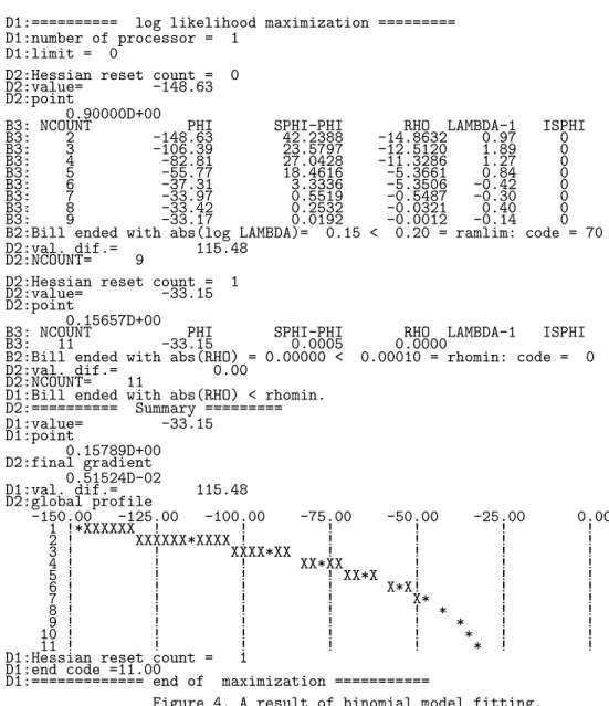
2(x−x_∗)^TV_n⁻¹(x−x_∗). (9) ﬁtted to the data is improved gradually. The position of the tangent point of the graph of(p) and the graph of the model isx_NCOUNT. Fig.3 and Fig.4 show the program and its output, respectively.

(6)

log l

0.0 0.2 0.4 0.6 0.8 1.0

-200 -150 -100 -50

onedim

log l

0.0 0.2 0.4 0.6 0.8 1.0

-200 -150 -100 -50

log l

0.0 0.2 0.4 0.6 0.8 1.0

-200 -150 -100 -50

NCOUNT=11

log l

0.0 0.2 0.4 0.6 0.8 1.0

-200 -150 -100 -50

log l

0.0 0.2 0.4 0.6 0.8 1.0

-200 -150 -100 -50

NCOUNT=2

log l

0.0 0.2 0.4 0.6 0.8 1.0

-200 -150 -100 -50

log l

0.0 0.2 0.4 0.6 0.8 1.0

-200 -150 -100 -50

NCOUNT=3

log l

0.0 0.2 0.4 0.6 0.8 1.0

-200 -150 -100 -50

log l

0.0 0.2 0.4 0.6 0.8 1.0

-200 -150 -100 -50

NCOUNT=4

log l

0.0 0.2 0.4 0.6 0.8 1.0

-200 -150 -100 -50

log l

0.0 0.2 0.4 0.6 0.8 1.0

-200 -150 -100 -50

NCOUNT=5

log l

0.0 0.2 0.4 0.6 0.8 1.0

-200 -150 -100 -50

log l

0.0 0.2 0.4 0.6 0.8 1.0

-200 -150 -100 -50

NCOUNT=6

log l

0.0 0.2 0.4 0.6 0.8 1.0

-200 -150 -100 -50

log l

0.0 0.2 0.4 0.6 0.8 1.0

-200 -150 -100 -50

NCOUNT=7

log l

0.0 0.2 0.4 0.6 0.8 1.0

-200 -150 -100 -50

log l

0.0 0.2 0.4 0.6 0.8 1.0

-200 -150 -100 -50

NCOUNT=8

log l

0.0 0.2 0.4 0.6 0.8 1.0

-200 -150 -100 -50

log l

0.0 0.2 0.4 0.6 0.8 1.0

-200 -150 -100 -50

NCOUNT=9

Figure 2 Numerical maximization of the log likelihood of a binomial model.

implicit real*8 (a-h,o-z) parameter (ipmax=5)

dimension g(ipmax), vd(ipmax,ipmax+5) dimension a1(ipmax),step(ipmax) common /cmodel/ m,m1

external model0 m = 76

m1 = 12

do 1 i=1,ipmax 1 step(i) = 0.001d0

ip1=1

a1(1) = 0.9d0

call dall(model0,a1,ip1,el,g,vd,endc,step,0,3) stop

end

subroutine model0(par,np,el,lel) implicit real*8 (a-h,o-z)

common /cmodel/ m,m1 dimension par(np) lel = 0

di = par(1)

if(di .le. 0.d0) return if(di .ge. 1.d0) return

(7)

f = m1 * dlog(di) + (m-m1) * dlog(1.d0-di) lel=1

return end

Figure 3. Program for binomial model fitting.

D1:========== log likelihood maximization =========

D1:number of processor = 1 D1:limit = 0

D2:Hessian reset count = 0 D2:value= -148.63 D2:point

0.90000D+00

B3: NCOUNT PHI SPHI-PHI RHO LAMBDA-1 ISPHI

B3: 2 -148.63 42.2388 -14.8632 0.97 0

B3: 3 -106.39 23.5797 -12.5120 1.89 0

B3: 4 -82.81 27.0428 -11.3286 1.27 0

B3: 5 -55.77 18.4616 -5.3661 0.84 0

B3: 6 -37.31 3.3336 -5.3506 -0.42 0

B3: 7 -33.97 0.5519 -0.5487 -0.30 0

B3: 8 -33.42 0.2532 -0.0321 0.40 0

B3: 9 -33.17 0.0192 -0.0012 -0.14 0

B2:Bill ended with abs(log LAMBDA)= 0.15 < 0.20 = ramlim: code = 70 D2:val. dif.= 115.48

D2:NCOUNT= 9

0.15657D+00

B3: 11 -33.15 0.0005 0.0000

B2:Bill ended with abs(RHO) = 0.00000 < 0.00010 = rhomin: code = 0

D2:val. dif.= 0.00

D2:NCOUNT= 11

D1:Bill ended with abs(RHO) < rhomin.

D2:========== Summary =========

D1:value= -33.15 D1:point

0.15789D+00 D2:final gradient

0.51524D-02

D1:val. dif.= 115.48 D2:global profile

-150.00 -125.00 -100.00 -75.00 -50.00 -25.00 0.00

1 !*XXXXXX ! ! ! ! ! !

2 ! XXXXXX*XXXX ! ! ! ! !

3 ! ! XXXX*XX ! ! ! !

4 ! ! ! XX*XX ! ! !

5 ! ! ! ! XX*X ! ! !

6 ! ! ! ! X*X! ! !

7 ! ! ! ! X* ! !

8 ! ! ! ! ! * ! !

9 ! ! ! ! ! * ! !

10 ! ! ! ! ! * ! !

11 ! ! ! ! ! * ! !

D1:Hessian reset count = 1 D1:end code =11.00

D1:============= end of maximization ===========

Figure 4. A result of binomial model fitting.

3.2 Two-dimensional Optimization

This example gives a ‘bird’s eye view’ of the performance of DALL. The following function is an artiﬁcial function. Not a real log likelihood function.

f(x , y) =−1

2{r(x²+x+y)²+ (x²+ 3x+y)²} (10) Here,r= 40.0. The function takes the maximum value 0.0 at point B(0,0) shown in the top-left panel of Fig.5-1. The initial guess is taken at point A(−2.5,−3.0). Two contour curves in dotted line at 1.0 and 10.0 below the highest point are drawn in the ﬁgure.

(8)

-4 -3 -2 -1 0 1 2 3 -4

-3 -2 -1 0 1 2 3

-4 -3 -2 -1 0 1 2 3

A

-4 -3 -2 -1 0 1 2 3

B

-4 -3 -2 -1 0 1 2 3

real

-4 -3 -2 -1 0 1 2 3

NCOUNT=70

-4 -3 -2 -1 0 1 2 3

NCOUNT=49

C

-4 -3 -2 -1 0 1 2 3

NCOUNT=50

C

-4 -3 -2 -1 0 1 2 3

NCOUNT=51

C

-4 -3 -2 -1 0 1 2 3

D

-4 -3 -2 -1 0 1 2 3

NCOUNT=52

D

-4 -3 -2 -1 0 1 2 3

NCOUNT=53

-4 -3 -2 -1 0 1 2 3

NCOUNT=54

Figure 5-1. Search process by Davidon’s algorithm.

Character ‘C’ in the panel titled NCOUNT = 51, indicates the position of the pointx₅₁. The solid oval is the contour line at the level ofφ_∗−10.0 of the model(9) estimated based on information obtained up to this moment. The function value at pointx_∗, the center of the oval, is less that the value atx₅₁ and it turned out that this model is not good and x₅₂issetequaltox₅₁. The model is modiﬁed to get one shown the in ﬁgure titled NCOUNT

= 52, the function value at x_∗(D) is larger than that at x₅₂ and x₅₃issetequaltox_∗. Iterating this process (see Figs. 5-2 and 5-3), we get the result shown in the ﬁgure titled NCOUNT=70 at top-right panel. Two ovals in solid line in the fugure are contour lines at levels ofφ_∗−1.0 andφ_∗−10.0. It is clear that ﬁtting of the last model is poor globally in this case. But the local structure of the object function is captured by the model.

(9)

-4 -3 -2 -1 0 1 2 3 -4

-3 -2 -1 0 1 2 3

-4 -3 -2 -1 0 1 2 3

NCOUNT=55

-4 -3 -2 -1 0 1 2 3

NCOUNT=56

-4 -3 -2 -1 0 1 2 3

NCOUNT=57

-4 -3 -2 -1 0 1 2 3

NCOUNT=58

-4 -3 -2 -1 0 1 2 3

NCOUNT=59

-4 -3 -2 -1 0 1 2 3

NCOUNT=60

-4 -3 -2 -1 0 1 2 3

NCOUNT=61

-4 -3 -2 -1 0 1 2 3

NCOUNT=62

Figure 5-2. (continued)

The print out of DALL is shown in Figure 3. The “graph” composed of * and X at the end of the ﬁgure shows proﬁle of the object function along the line from point A to B. Since this “graph” does not show the function values at pointsx₁,x₂,. . .,it does not increase monotonically. Seeing this “graph” we can get some information if the object function has an easy shape or not.

(10)

-4 -3 -2 -1 0 1 2 3 -4

-3 -2 -1 0 1 2 3

-4 -3 -2 -1 0 1 2 3

NCOUNT=63

-4 -3 -2 -1 0 1 2 3

NCOUNT=64

-4 -3 -2 -1 0 1 2 3

NCOUNT=65

-4 -3 -2 -1 0 1 2 3

NCOUNT=66

-4 -3 -2 -1 0 1 2 3

NCOUNT=67

-4 -3 -2 -1 0 1 2 3

NCOUNT=68

-4 -3 -2 -1 0 1 2 3

NCOUNT=69

-4 -3 -2 -1 0 1 2 3

NCOUNT=70

Figure 5-3. (continued) D2:Hessian reset count = 11

D2:value= -7.60

D2:point

-0.19124D+01 -0.15012D+01

B3: 47 -7.60 0.1857 -2.2604 -0.50 0

B3: 48 -7.41 0.6270 -0.0819 2.73 0

B3: 49 -6.79 0.2991 -0.2897 3.00 0

B3: 50 -6.49 1.1112 -0.9496 3.00 0

B3: 51 -5.38 -1.0834 -49.6538 -0.75 0

B3: 52 -5.38 1.3701 -1.0523 3.00 0

B3: 53 -4.01 -8.7070 -390.8665 -0.75 0

B3: 54 -4.01 1.0407 -0.5745 2.85 0

B3: 55 -2.97 -2.2384 -73.4456 -0.75 1

B3: 56 -2.97 0.7719 -0.4114 2.26 0

B3: 57 -2.19 0.2893 -4.6355 -0.75 0

B3: 58 -1.90 0.4668 -0.3263 -0.75 0

B3: 59 -1.44 0.0776 -0.0683 3.00 0

B3: 60 -1.36 0.2411 -0.1684 3.00 0

B3: 61 -1.12 0.4728 -0.2189 3.00 0

B3: 62 -0.65 0.0453 -3.1124 -0.75 0

B3: 63 -0.60 0.3932 -0.0996 -0.71 0

B3: 64 -0.21 0.0271 -0.0233 3.00 0

B3: 65 -0.18 0.0763 -0.0422 2.51 0

B3: 66 -0.10 0.0882 -0.0166 0.92 0

B3: 67 -0.02 0.0025 -0.0915 -0.75 0

B3: 68 -0.01 0.0123 -0.0015 3.00 0

B3: 69 0.00 -0.0001 -0.0065 -0.52 0

B3: 70 0.00 0.0014 0.0000

(11)

D2:val. dif.= 7.60 D2:NCOUNT= 70

D2:========== Summary =========

D1:value= 0.00

D1:point

-0.97975D-06 -0.80570D-03 D2:final gradient

0.34650D-01 0.33076D-01 D1:val. dif.= 20.28 D2:global profile

-40.00 -30.00 -20.00 -10.00 0.00 10.00

1 ! ! *XXXXX ! ! !

2 ! ! ! XXXXX* ! !

3 ! ! ! XXXXX*X ! ! !

4 ! ! XXXX*XXXXX ! ! !

5 ! XX*XXXX ! ! ! !

6 ! *XX ! ! ! ! !

7 ! *XXXX! ! ! ! !

8 ! XXXX*XXXXXX ! ! ! !

9 ! ! XXXXXX*XXXXXX! ! !

10 ! ! ! XXXXXX*XX ! !

11 ! ! ! ! XX* !

Figure 6Output of DALL

3.3 Constrained Gaussian model fitting

Letx₁,. . ., x_n be data. The log likelihood of a normal distribution model with respect to the data is given by

l_x(µ_x, σ²_x) =−n

2 log 2π−n

2logσ²_x− 1 2σ_x²

nx

i=1

(x_i−µ_x)². (11) For datay₁,. . ., y_n;

l_y(µ_y, σ_y²) =−n

2log 2π−n

2 logσ_y²− 1 2σ_y²

ny

i=1

(y_i−µ_x)². (12) MLE’s ofµ_xandσ²_xare

µˆ_x= 1 n

n

i=1

x_i and

σˆ²_x= 1 n_x

nx

i=1

(x_i−µˆ_x)², Similar expression forµ_y, σ_y²can be given.

For data x = {0.73,−0.06,1.04,2.29,0.51,−0.45,1.03,0.44,0.02,0.11,−2.42} MLE’s are

µˆ_x = 0.2945 ˆσ_x² = 1.2267

and MLE’s for datay={0.10,0.56,−1.11,−0.48,3.46,−2.39,0.36,4.56}are µˆ_y = 0.6325

ˆσ_y² = 4.6491.

The log likelihood for the model with the constraintµ_x=µ_y is given by l_x+y(µ_x+y, σ²_x, σ_y²) = −n

2 log 2π−n

2logσ_x²− 1 2σ_x²

nx

i=1

(x_i−µ_x+y)²

−n

2 log 2π−n

2logσ_y²− 1 2σ²_y

ny

i=1

(y_i−µ_x+y)²

(12)

The problem of analytical maximization of the function is equvalent to solving an algebraic equation of order three. Instead, let DALL solve the problem. Prepare subroutines shown in Fig.7.

Subroutinesllx,llyandllxy, are composed so that they compute log likelihood for parameter value speciﬁes by the arraypof lengthm. As eq.(13) show the subroutinllxy is composed so that it calls llx and lly. The main routine and results aare shown as Figures 8 and 9, respectively. From the resultant relation

AICx+AICy= 37.46 + 39.00 = 76.46>74.62 =AICxy supports the assumptionµ_x=µ_y.

subroutine llx(p,m,el,lel) implicit real*8 (a-h,o-z) dimension p(m)

common /i721/ n common /r721/ x(11) data pi /3.14159265d0/

lel=0

if(p(2) .gt. 0.d0) then sum=0.d0

do 1 i=1,n

sum=sum+(x(i)-p(1))**2 1 continue

el= -n*0.5*( dlog(pi*2)+dlog(p(2)) ) - 0.5*sum/p(2) lel=1

end if return c end

subroutine lly(p,m,el,lel) implicit real*8 (a-h,o-z) dimension p(m)

common /i722/ n common /r722/ x(8) data pi /3.14159265d0/

lel=0

if(p(2) .gt. 0.d0) then sum=0.d0

do 1 i=1,n

sum=sum+(x(i)-p(1))**2 1 continue

el= -n*0.5*( dlog(pi*2)+dlog(p(2)) ) - 0.5*sum/p(2) lel=1

end if return end c

subroutine llxy(p,m,el,lel) implicit real*8 (a-h,o-z) dimension p(m),px(2),py(2) px(1)=p(1)

px(2)=p(2)

call llx(px,2,elx,lel) if(lel .eq. 0) return py(1)=p(1)

py(2)=p(3)

call lly(py,2,ely,lel) if(lel .eq. 0) return el=elx+ely

return c end

block data ex72

implicit real*8 (a-h,o-z) common /i721/ n1

common /r721/ x1(11) common /i722/ n2 common /r722/ x2(8) data n1/11/

data x1/ 0.73, -0.06, 1.04, 2.29, 0.51,

* -0.45, 1.03, 0.44, 0.02, 0.11,

* -2.42 /

data n2/8/

data x2/ 0.10, 0.56, -1.11, -0.48, 3.46,

* -2.39, 0.36, 4.56 / end

Figure 7. Subroutines to compute log likelihood of Gaussian models and constrained Gaussian model.

parameter (ipmax=4) implicit real*8( a-h,o-z )

(13)

dimension ax(ipmax),ay(ipmax),axy(ipmax)

dimension g(ipmax), vd(ipmax,ipmax+5),step(ipmax) external llx,lly,llxy

c myid = 0 do 1 i=1,ipmax 1 step(i) = 0.001d0

ipx=2 ax(1) = 0.d0 ax(2) = 1.d0

call dall(llx,ax,ipx,el,g,vd,endc,step,0,3) if(myid .eq. 0) then

write(6,*) ’ meanx(mle)=’,ax(1) write(6,*) ’ variancex(mle)=’,ax(2) write(6,*) ’ maximum likelihood=’,el write(6,*) ’ number of parameter=’,ipx aic= -2*el + 2*ipx

write(6,’(’’ AICx=’’,F10.2)’) aic end if

ipy=2 ay(1) = 0.d0 ay(2) = 1.d0

call dall(lly,ay,ipy,el,g,vd,endc,step,0,3) if(myid .eq. 0) then

write(6,*) ’ meany(mle)=’,ay(1) write(6,*) ’ variancey(mle)=’,ay(2) write(6,*) ’ maximum likelihood=’,el write(6,*) ’ number of parameter=’,ipy aic= -2*el + 2*ipy

write(6,’(’’ AICy=’’,F10.2)’) aic end if

ipxy=3

axy(1) = (ax(1) + ay(1))*0.5d0 axy(2) = ax(2)

axy(3) = ay(2)

call dall(llxy,axy,ipxy,el,g,vd,endc,step,0,3) if(myid .eq. 0) then

write(6,*) ’ meanxy(mle)=’,axy(1) write(6,*) ’ variancedx1(mle)=’,axy(2) write(6,*) ’ variancey(mle)=’,axy(3) write(6,*) ’ maximum likelihood=’,el write(6,*) ’ number of parameter=’,ipxy aic= -2*el + 2*ipxy

write(6,’(’’ AICxy=’’,F10.2)’) aic end if

stop end

Figure 8. A main program to fit Gaussian distribution model and constrained Gaussian distribution model.

0.00000D+00 0.10000D+01

B3: 2 -17.33 0.5980 -0.0019 0.08 0

B2:Bill ended with abs(log LAMBDA)= 0.08 < 0.20 = ramlim: code = 70

D2:val. dif.= 0.60

D2:NCOUNT= 2

0.29455D+00 0.11927D+01

B3: 5 -16.73 0.0022 0.0000

D2:val. dif.= 0.00

D2:NCOUNT= 5

D2:========== Summary =========

0.29455D+00 0.12249D+01 D2:final gradient

-0.17764D-11 0.67384D-02

D1:val. dif.= 0.60

D2:global profile

-17.50 -17.25 -17.00 -16.75 -16.50 -16.25 -16.00

1 ! *XX! ! ! ! ! !

2 ! XX*X ! ! ! ! !

3 ! ! X*X ! ! ! ! !

(14)

6 ! ! ! * ! ! ! !

7 ! ! ! * ! ! ! !

8 ! ! ! *! ! ! !

9 ! ! ! * ! ! !

10 ! ! ! !* ! ! !

11 ! ! ! !* ! ! !

D1:Hessian reset count = 1 D1:end code = 4.00

meanx(mle)= 0.29454545454562 variancex(mle)= 1.2248781111300 maximum likelihood= -16.732202448716 number of parameter= 2

AICx= 37.46

0.00000D+00 0.10000D+01

B3: 2 -27.55 5.8549 -1.0351 0.61 0

B3: 3 -21.69 1.3469 -0.7011 1.85 0

B3: 4 -20.35 1.4235 -0.4922 0.99 0

B3: 5 -18.92 0.7238 -0.2774 1.14 0

B3: 6 -18.20 0.4243 -0.1402 0.95 0

B3: 7 -17.77 0.1914 -0.0559 0.83 0

B3: 8 -17.58 0.0684 -0.0149 0.62 0

B3: 9 -17.51 0.0151 -0.0019 0.39 0

B3: 10 -17.50 0.0015 -0.0001

B2:Bill ended with abs(RHO) = 0.00006 < 0.00010 = rhomin: code = 0 D2:val. dif.= 10.05

D2:NCOUNT= 10

D2:========== Summary =========

0.63250D+00 0.46284D+01 D2:final gradient

-0.44409D-10 0.38577D-02 D1:val. dif.= 10.05 D2:global profile

-30.00 -27.50 -25.00 -22.50 -20.00 -17.50 -15.00

1 ! *XXXXXXXX ! ! ! ! !

2 ! ! XXXXXXXX*XXXX ! ! !

3 ! ! ! ! XXXX*XX ! ! !

4 ! ! ! ! XX*X ! !

5 ! ! ! ! ! X* ! !

6 ! ! ! ! ! * ! !

7 ! ! ! ! ! * ! !

8 ! ! ! ! ! *! !

9 ! ! ! ! ! * !

10 ! ! ! ! ! * !

11 ! ! ! ! ! * !

meany(mle)= 0.63250000002579 variancey(mle)= 4.6284090071286 maximum likelihood= -17.498215714685 number of parameter= 2

AICy= 39.00

0.46352D+00 0.12249D+01 0.46284D+01

B3: 2 -34.38 0.0698 -0.0023 -0.47 0

B3: 3 -34.31 0.0009 -0.0003 1.09 0

B3: 4 -34.31 0.0003 0.0000

D2:val. dif.= 0.07

D2:NCOUNT= 4

D2:========== Summary =========

0.34827D+00 0.12291D+01 0.47291D+01 D2:final gradient

0.22816D-04 0.19078D-02 0.14178D-03

D1:val. dif.= 0.07

D2:global profile

-34.50 -34.25 -34.00 -33.75 -33.50 -33.25 -33.00

1 ! * ! ! ! ! ! !

2 ! * ! ! ! ! ! !

3 ! * ! ! ! ! ! !

4 ! * ! ! ! ! ! !

5 ! * ! ! ! ! ! !

6 ! * ! ! ! ! ! !

7 ! * ! ! ! ! ! !

8 ! * ! ! ! ! ! !

9 ! * ! ! ! ! ! !

10 ! * ! ! ! ! ! !

11 ! * ! ! ! ! ! !

D1:Hessian reset count = 0 D1:end code = 4.00

meanxy(mle)= 0.34826773312855 variancex(mle)= 1.2290783247532 variancey(mle)= 4.7290641711741 maximum likelihood= -34.312209336033 number of parameter= 3

AIC3= 74.62

(15)

Figure 9. Fitting of Gauss model and constrained Gauss model.

4 Distributed files

DALL package summarized in Table 5 can be obtained at http://www.ism.ac.jp/software/ismlib/soft.e.html

Table 5. ARdock package ﬁle name contents

README Latest announcement

example3.f log likelihood subroutines and main program for the third example and DALL routine in FORTRAN

gauss.c log likelihood subroutines and main program for the third example in C dall pack.c DALL routine in C

nrutil.h a headder ﬁle required by dall pack.c

Makefile sample makefile for C version for Unix environment dall.ps post script file of this monograph

Note: FORTRAN version DALL routine contained in this ﬁle is the one extracted from ARdock package. Those users who are interested in using DALL on a parallel computer are invited to down-load the source code of ARdock package.

ARdock, an Auto-Regressive model analyzer

Copiright_OML 1999Makio Ishiguro, Hiroko Kato & Hirotugu Akaike (http://www.ism.ac.jp/software/ismlib/soft.e.html)

So far, the test of DALL is successfully done in environments summarized in the following Table.

Table 6. Computation Environments

Hardware Operating System Compiler

HITACHI SR8000 HI-UX/MPP FORTRAN90

HP9000V2250 HP-UX 11.0 HP Fortran 90

IBM R/6000 SP AIX Version 4 AIX XL Fortran

SGI Origin 2000/4-DS-I IRIX Release 6.4 IP27 FORTRAN90 SPARCstation 5 Sun OS 4.1.4-JLE 1.1.4 g77 version0.5.23

PC-9801 nx/C MS-DOS 5.00A-H Microsoft FORTRAN Version 4.01

4.1 Licencing policy

We make public the source code of DALL under the open market licence policy proposed by the Institute of Statistical Mathematics.

Open Market Licence for software(version:OML-SW-E-1996)

0. In the following, “Copyright OML notice” means “the copyright notice with a statement saying that the said software is made public under this Open Market Licence for software”.

1. On the condition that “Copyright OML notice” and attached statements are copied as they are, all or any portion of the said software can be copied or redistributed.

2. Modification of the software is permitted, provided that the exact place of the modification, the date and the name of the modifier are shown conspicuously.

3. It is forbidden to apply for a patent on the software which utilizes the said software.

(16)

4. The said software is distributed without any warranty. The copyright holder takes no responsibility for any damage caused by the use of the said software.

5. Any interactively controlled application made utilizing the said software has to show “Copyright OML notice” and attached statements conspicuously when it is started up.

For the healthy development of software science, suitable form of the licencing is important. We definitely would like to claim our copyright to DALL. And we would like to use our copyright to let all concerned people use DALL source code freely under two conditions that (1) our credit is properly referred and (2) statements attached to the copyright note saying that the original DALL source code is distributed from the specified site without charge are kept as they are. We permit modification or redistribution of DALL source code as far as these two conditions are met. The redistribution may be with or without charge.

[Recommended form of reference/acknowledgment] When you are to publish software xxxxx, which utilizes DALL, here is an example of making reference to DAL- L.

xxxxx Copyright, 20yy uuuuu

xxxxx utilizes DALL, with here and there modiﬁcations. The places of modi- ﬁcations are indicated in the code.

DALL A subroutine for statistical model builders Copyright OML, 1996, 1999 M. Ishiguro and H. Akaike

The source code of this software can be obtained from ISMLIB⁽¹⁾ of the In- stitute of Statistical Mathematics without any charge. On the conditions that terms of the OPEN MARKET LICENCE⁽²⁾for software are observed and that the copyright holder nor the Institute of Statistical Mathematics take no responsibility on any result from the use, the program can be used or modiﬁed freely. On the condition that this note is attached as it is, DALL can be redistributed.

(1) http://www.ism.ac.jp/software/ismlib/soft.e.html (2) ftp://ftp.ism.ac.jp/pub/ISMLIB/OML/OML-SW-E-1996

5 Acknowledgement

A part of this work is supported by the Grant-in-Aid for Scientiﬁc Research provided by The Ministry of Education, Science and Culture. Conversion of FORTRAN version DALL to C version was done by Mr. Yasumasa Matsuda of Kanagawa University. We would like to thank Ms.Syeda shahanra Hug of the Graduate University for Advanced Studies for her comments of the text.

References

[1] Akaike, H. (1973) Information theory and an etension of the maximum likelihood prin- ciple,2nd International Symposium on Information Theory(Petrov, B. N. and Csaki, F. eds.), Akademiai Kiado, Budapest, pp.267–281. (Reproduced in Breakthroughs in Statistics, volume 1, S.Kotz and N. L. Johnson, eds., Springer Verlag, New York, (1992).)

[2] Akaike, H., Arahata, E. & Ozaki, T. (1975). TIMSAC-74: A time series analysis and control program package - (1) & (2),Computer Science Monographs No.5 & No.6, The institute of Statistical Mathematics, Tokyo.

[3] Davidon, W.C. (1968). Variance Algorithm for Minimization,Computer Journal, 10, 406-410.

(17)

[4] Isiguro, M., Hiroko, Kato and Akaike, H.(1999). ARdock, an Auto-Regressive model analyzer,Computer Science Monographs No.30, The institute of Statistical Mathemat- ics, Tokyo.

[5] Douke, H. & Asano, Ch. (1989). Developmental study of a maximum likelihood estimation system: MLE-SYS, inProceedings of the sixth Korea and Japan joint conference of statistics held in Pusan, Korea, July 10-12, 1989, pp.134-145.

[6] Kowalik, J. & Osborne, M.R. (1968).Methods for unconstrained optimization problems, American Elsevier Publishing Co. Inc., New York.

[7] K¨unzi, H.P. Tzschach, H.G. & Zehnder, C.A. (1968),Numerical methods of mathemat- ical optimization, Academic Press, New York.

[8] Lavi, A. & Vogl, T.P. (1966),Recent advances in optimization techniques, John Wiley

& Sons, Inc., New York.

[9] Powell, M.J.D. (1981). Nonlinear Optimization 1981, Academic Press, London/New York.

[10] Sakamoto, Y., Ishiguro, M. & Kitagawa, G. (1986). Akaike Information Criterion Statistics, D.Reidel Publishing Company, Dordrecht/Tokyo.