Vol. XXII (September 1984), pp. 1007-1051
Applied General-Equilibrium Models of Taxation and International Trade:
An Introduction and Survey
By JOHN B. SHOVEN Stanford University and National Bureau of Economic Research
and JOHN WHALLEY University of Western Ontario
We wish to acknowledge the help of three referees and of John Pencavel on several earlier drafts, as well as the assistance of the modelers, whose work is referred to in the paper. They corrected our lack of understanding of their work and provided many other helpful comments.
Excellent research and bibliographical assistance have been pro- vided by Debbie Fretz, Radwan Shaban, and Janet Stotsky. Helpful comments have been made by Charles Ballard, Michael Boskin, Lans Bovenberg, Sylvester Damus, Harvey Galper, Glenn Harrison, Gor- don Lenjosek, Jack Mutti, Serena Ng, T. N. Srinivasan, Charles Stuart, and Eric Toder. The authors also acknowledgefinancial sup- port from the National Bureau of Economic Research, the National Science Foundation, International Business Machines, and the Social Sciences and Humanities Research Council: Ottawa, Canada.
I. Introduction
THE BODY OF RESEARCH discussed here is part of a wider series of develop- ments which, in the last few years, has become known as "applied general-equi- librium analysis." The explicit aim of this literature is to convert the Walrasian gen- eral-equilibrium structure (formalized in the 1950s by Kenneth Arrow, Gerard De- breu, and others) from an abstract repre- sentation of an economy into realistic models of actual economies. The idea is
to use these models to evaluate policy op- tions by specifying production and de- mand parameters and incorporating data reflective of real economies. Most contem- porary applied general-equilibrium mod- els are numerical analogs of traditional two-sector general-equilibrium models that James Meade, Harry G. Johnson, Ar- nold Harberger, and others popularized in the 1950s and 1960s. Earlier analytic work with these models has examined the distortionary effects of taxes, tariffs and other policies, along with functional inci- 1007
1008 Journal of Economic Literature, Vol. XXII (September 1984) dence questions. Recent applied models,
surveyed here, provide numerical esti- mates of efficiency and distributional ef- fects within the same framework.
The Walrasian model provides an ideal framework for appraising the effects of policy changes on resource allocation and for assessing who gains and loses, policy impacts not well covered by empirical macro models. We discuss a number of ways in which these models are already providing fresh insights into long-standing policy controversies. Due to space con- straints, we will limit our discussion to re- cent modeling efforts in the fields of taxa- tion and international trade.
The value of these computational mod- els is that a computer removes the need to work in small dimensions: Much more detail and complexity can be incorporated than in simple analytic models. For in- stance, tax policy models can simulta- neously accommodate several taxes. This is important because taxes compound in effect with other taxes even when evaluat- ing changes in only one tax. Models involv- ing 30 or more sectors and industries are commonly employed, providing substan- tial detail for policymakers concerned with feedback effects of policy initiatives directed only at specified products or in- dustries.
The models reported here extend Was- sily Leontiefs work on empirical Walra- sian models based on fixed input-output coefficients by incorporating substitution effects in both production and demand, and by including more than one con- sumer. Earlier work by three economists provides background for much of this ac- tivity. One is Leif Johansen (1960) who formulated the first empirically based, multi-sector, price-endogenous model an- alyzing resource allocation issues. He ap- plied this model to policy questions in Norway. Another is Arnold Harberger (1962), who was the first author to investi- gate tax policy questions numerically in a two-sector general-equilibrium frame-
work. A final important source of stimulus has been an ingenious computer algo- rithm for the numerical determination of the equilibrium of a Walrasian system, de- veloped by Herbert Scarf in 1967. Despite subsequent extensions to his original al- gorithm, and more recently the use of al- ternative solution techniques, Scarfs work has been instrumental in persuading some of the recent generation of mathemati- cally-trained economists to approach gen- eral equilibrium from a computational and, ultimately, a practical perspective.
Applied general-equilibrium tax models have been used to analyze such policy ini- tiatives as integrating personal and corpo- rate taxes, the introduction of value-added taxes, and indexing the tax system. In in- ternational trade models the impacts of trade policy changes on resource alloca- tion within countries, custom union issues, international trade negotiations under the GATT, and North-South trade questions have been analyzed.
The plan of this paper is as follows: Sec- tion 2 presents a simple numerical exam- ple designed to illustrate how applied gen- eral-equilibrium models operate; Section 3 discusses how the methods illustrated by the numerical example can be imple- mented (the choice of parameter values and functional forms, the use of data, solu- tion methods, and how policy conclusions are formulated); Section 4 presents the main features of recent tax models and highlights their most important policy im- plications; Section 5 similarly discusses trade models; we close with an evaluation of the approach and outline what could be useful directions for further research in this area.
II. What Is Applied General-Equilibrium Analysis?
Applied general-equilibrium analysis in- volves using a numerically specified gen- eral-equilibrium model for policy evalua- tion. However, despite the widespread
use of the term "general equilibrium" in modern economics, the precise meaning of the term is often not fully defined. Ev- eryone seems to agree that a general-equi- librium model is one in which all markets clear in equilibrium; there seems to be less agreement as to the essential elements of structure which underlie the equilib- rium formulation.
Our use of the term corresponds to the well-known Arrow-Debreu model, elabo- rated on in Arrow and F. H. Hahn (1971).
The number of consumers in the model is specified. Each of them has an initial endowment of the N commodities and a set of preferences, resulting in demand functions for each commodity. Market demands are the sum of each consumer's demands. Commodity market demands depend on all prices, are continuous, non- negative, homogeneous of degree zero (i.e., no money illusion) and satisfy Walras' Law (i.e., that at any set of prices, the total value of consumer expenditures equals consumer incomes). On the production side, technology is described by either constant returns to scale activities or non- increasing returns to scale production functions. Producers maximize profits.
The zero homogeneity of demand func- tions and the linear homogeneity of profits in prices (i.e., doubling all prices doubles money profits) implies that only relative prices are of any significance in such a model; the absolute price level has no im- pact on the equilibrium outcome.
Equilibrium in this model is character- ized by a set of prices and levels of produc- tion in each industry such that market de- mand equals supply for all commodities (including disposals if any commodity is a free good). Since producers are assumed to maximize profits, this implies that in the constant-returns-to-scale case no activ- ity (or cost-minimizing techniques for pro- duction functions) does any better than break even at the equilibrium prices.
To illustrate how these models work, we present a simplified numerical example
representative of those actually used to analyze policy issues. We consider a model with two final goods (manufacturing and nonmanufacturing), two factors of produc- tion (capital and labor), and two classes of consumers. Consumers have initial en- dowments of factors, but have no initial endowments of goods. A "rich" consumer group owns all the capital, while a "poor"
group owns all the labor. Production of each good takes place according to a con- stant-returns-to-scale, constant-elasticity- of-substitution (CES) production function, and each consumer class has commodity demand functions generated by maximiz- ing a CES utility function subject to its budget constraint. There are no consumer demands for factors (i.e., no labor-leisure choice). Even though the two consumer- two producer nature of this example means that it is similar to the Harberger (1962) tax model and could be solved ana- lytically, the solution techniques used here are applicable to larger and more sophisticated models.
The production functions for the exam- ple are given by
Qi=4 LiL, 1 (1)
1 (2-1)]
+ (1 -8i)Ki C , i=1,2 where Qi denotes output of the ith indus- try, 4i is the scale or units parameter, FJ is the distribution parameter, Ki and L.
are the capital and laborfactor inputs, and vi is the elasticity of factor substitution.
The factor demand functions derived from cost minimization for these produc- tion functions (1) are:
L4 = 4l'Qi [i
] fi (2)
+ (1 1_ 8i) 3Z)PL jJ(li)J (1 -
1010 Journal of Economic Literature, Vol. XXII (September 1984) and,
O'i
(1- i) where PK and PL are the per-unit factor costs for the industry (including factor taxes if applicable).
The CES utility functions are given by
- 1 (Cc-1) - C
2 CC (CC ((CC-1 (4) where Xc is the quantity of good i de- manded by the Cth consumer, ac are share parameters, and oc is the substitution elas- ticity in consumer c's CES utility function.
The consumer's budget equation is P1X
? P2X2 < PL WL + PK WK = IC, where P1 and P2 are the consumer prices for the two output commodities, WL and WK are consumer c's endowment of labor and capital, and IC is the income of consumer c. If this utility function is maximized, sub- ject to the budget constraint, the demand functions are:
c~ = a- icIc
picc (acP l - cC) + acpl - crc)) (5) i 1, 2; c = 1, 2.
In this simple model, there are ten param- eters whose values need to be specified:
six production function parameters which affect the supply of the two products (i.e., (P, 8s, and cr- for i = 1, 2), and four utility function parameters determining the de- mand for each of the two products by each of the two consumers (i.e., al, a2, ,r1, and 0c2). There are four exogenous variables whose values must also be specified: the endowment of labor (WL) and capital (WK)
for each of the two consumers. The solu- tion to the model is characterized by 12
variables, the four prices P1, P2, PL, PK,
and the eight quantities Xl, X2, Xl, X2, and K1, K2, L1, L2 which meet the re- quired conditions for equilibrium.
The equilibrium conditions in this model are that market demand equals market supply for all inputs and outputs, and that profits are zero in each industry.
These can be written out more fully as:
(a) Demands equal supply for factors
Ki(PL, PK, Qi) (6
+ K2(PL, PK, Q2)=K
Li(PL, PK, Qi) (7
+ L2(PL, PK, Q2) = ( where K1(PL, PK, Qi), K2(PL, PK, Q2), L1(PL, PK, Qi) and L2(PL, PK, Q2) are given by (2) and (3).
(b) Demands equal supply for goods Xl (P1, P2, PL, PK) (8)
+X (P1, P2, PL, PK) = Q ( Xl (P1, P2, PL, PK)
+ X2(P1, P2, PL, PK) = Q2 where Xl, Xi, X2, and X2, are given by maximizing (4), subject to consumer bud- get constraints, and Q1 and Q2 are given by (1). Finally, we have:
(c) Zero profit conditions hold in both industries
PKKi(PL, PK, Qi) (10)
+ PLL1(PL, PK, Qi) = P1Q1
PKK2(PL, PK, Q2)
+ PLL2(PL, PK, Q2) = P2Q2.
Given the four commodity and factor prices, one can evaluate the demands for commodities by all consumers because factor prices determine consumer in- comes (which give the position of each consumer's budget constraint), and com- modity prices give the slope of the budget
constraint. The factor requirements to meet commodity demands are given by (2) and (3). An equilibrium is therefore characterized by four prices, PL, PK, Pl,
P2, such that equations (6)-(11) hold.
Once the parameters of these produc- tion and demand functions are specified and the factor endowments are known, a complete general-equilibrium model is available. Tax and other policy variables can then be added as desired.
By way of example, in Table 1 we list sample numerical values for all the param- eters and the exogenous variables in this model. We have then solved this example using Olin Merrill's (1972) fixed-point al- gorithm, a refinement of the Scarf algo- rithm. This algorithm finds a set of market clearing prices for goods and factors, pro- viding a solution to the simultaneous non- linear equations above, (6)-(11).
The equilibrium solution for this exam- ple (the values of the endogenous varia- bles) is shown in Table 2. At the computed set of equilibrium prices, total demand for each output exactly matches the amount produced, and producer revenues equal consumer expenditures. Labor and capital endowments are fully employed, and con- sumer factor incomes equal producer fac- tor costs. Because of our assumption of constant returns to scale, the per-unit cost in each industry equals the selling price, meaning that economic profits are zero.
The expenditures of each household ex- haust its income. Since only relative prices affect behavior in general-equilibrium models such as this, we have chosen labor as numeraire.
To illustrate how a general-equilibrium model can be adapted for policy evalua- tion work, we consider the same numeri- cal example as above, but with a tax policy regime added using the approach as in Shoven and Whalley (1973). The funda- mental difficulty in modifying the model to incorporate taxes is the interdepen- dence of demands and supplies, and tax
TABLE 1
SPECIFICATION OF PRODUCTION PARAMETERS, DEMAND PARAMETERS, AND ENDOWMENTS FOR
A SIMPLE GENERAL-EQUILIBRIUM MODEL
Sector Production Parame-
ters
(Di 8i O'i
Manufacturing 1.5 .6 2.0
Nonmanufacturing 2.0 .7 .5
Demand Parameters
Rich Consumers Poor Consumers
ac a c qC ac aL c C c
0.5 0.5 1.5 0.3 0.7 0.75
Endowments
K L
Rich Households 25 0
Poor Households 0 60
revenues. For a given tax program (that is, for a specified tax rate imposed on a particular commodity or factor) tax reve- nues will be determined once demands, production levels, and factor employ- ments are known. Demands also depend on tax proceeds since these provide in- come to one or more of the agents in the economy. The solution suggested by Sho- ven and Whalley is to solve not only for equilibrium prices as in the example above, but also for equilibrium tax reve- nues. In the simple case where all govern- ment revenues are redistributed to con- sumers (i.e., no provision of public goods and services), this means that in equilib- rium the transfer payments made by gov- ernment to consumers equal taxes col- lected by government. This is another condition that the equilibrium must sat- isfy.
We assume the same values of the pa- rameters and exogenous variables as given in Table 1, along with an exogenously specified tax rate of 50 percent on each unit of capital income generated in the manufacturing sector. In the disburse-
1012 Journal of Economic Literature, Vol. XXII (September 1984)
TABLE 2
EQUILIBRIUM SOLUTION FOR ILLUSTRATIVE SIMPLE No TAX GENERAL-EQUILIBRIUM MODEL (PARAMETER VALUES SPECIFIED IN TABLE 1)
Equilibrium Prices
Manufacturing Output 1.399
Nonmanufacturing Output 1.093
Capital 1.373
Labor 1.000
Production
Quantity Revenue Capital Capital Cost
Manufacturing 24.942 34.898 6.212 8.532
Nonmanufacturing 54.378 59.439 18.788 25.805
Total 94.337 25.000 34.337
Cost Per
Labor Labor Cost Total Cost Unit Output
Manufacturing 26.366 26.366 34.898 1.399
Nonmanufacturing 33.634 33.634 59.439 1.093
Total 60.000 60.000 94.337
Demands
Manufacturing Nonmanufacturing Expenditure
Rich Households 11.514 16.674 34.337
Poor Households 13.428 37.704 60.000
Total 24.942 54.378 94.337
Labor Income Capital Income Total Income
Rich Households 0 34.337 34.337
Poor Households 60.000 0 60.000
Total 60.000 34.337 94.337
ment of tax revenues, we assume that rich households receive 40 percent, with the remaining 60 percent going to poor households. The new equilibrium solu- tion is shown in Table 3.
It is useful to illustrate how a general- equilibrium calculation differs from other less satisfactory methods. One purpose of such an equilibrium calculation might be to calculate the tax revenues that accrue to government from the taxes. A naive revenue estimate might use the equilib-
rium values in Table 2 as the base for the tax. In the no-tax regime the price of capi- tal is 1.373 and the employment of capital in manufacturing is 6.212. A 50 percent tax rate on capital income in manufactur- ing might therefore be expected to raise 4.265 units of revenue (i.e., 50 percent of 1.373 x 6.212). In fact, this would be a seriously misleading estimate of tax reve- nues. When all the general-equilibrium responses are allowed for, the new reve- nue is only 2.278. Compared with the no-
TABLE 3
EQuILIBRIUM SOLUTION FOR ILLUSTRATIVE SIMPLE GENERAL-EQuILIBRIUM MODEL WITH 50%
TAX ON MANUFACTURING CAPITAL
Equilibrium Prices
Manufacturing Output 1.467
Nonmanufacturing Output 1.006
Capital 1.128
Labor 1.000
Production
Capital Cost
Quantity Revenue Capital (including tax)
Manufacturing 22.387 32.830 4.039 6.832
Nonmanufacturing 57.307 57.639 20.961 23.637
Total 90.469 25.000 30.469
Cost Per
Labor Labor Cost Total Cost Unit Output
Manufacturing 25.999 25.999 32.831 1.467
Nonmanufacturing 34.001 34.001 57.638 1.006
Total 60.000 60.000 90.469
Demands
Manufacturing Nonmanufacturing Expenditure
Rich Households 8.989 15.827 29.102
Poor Households 13.398 41.480 61.367
Total 22.387 57.307 90.469
Labor Income Capital Income Transfers Total Income
Rich Households 0 28.191 .911 29.102
Poor Households 60.000 0 1.367 61.367
Total 60.000 28.191 2.278 90.469
tax equilibrium, the relative price of man- ufacturing to nonmanufacturing output rises, while the net-of-tax price of capital falls. However, the tax-inclusive cost of capital in manufacturing increases, lead- ing to a less capital-intensive method of production in manufacturing. Less manu- facturing and more nonmanufacturing output is produced because of the tax.
Expenditures of "poor" (labor-owning) households increase, while those of "rich"
(capital-owning) households fall. General-
equilibrium effects, therefore, need to be taken into account in revenue estimation, or in any other policy issue arising from such a tax.
A question frequently addressed by these models is whether any particular policy change is welfare-improving. In this instance, policy appraisal using these techniques usually relies upon a compari- son between an existing equilibrium (i.e., with unchanged tax policies), and a coun- terfactual equilibrium computed with
1014 Journal of Economic Literature, Vol. XXII (September 1984) modified policies. Because the underlying
theoretical structure of these models is so firmly rooted in traditional microtheory, a common procedure is to construct nu- merical welfare measures of the gain or loss.
The measures most widely employed are Hicksian compensating and equiva- lent variations associated with the equilib- rium comparison. The compensating vari- ation (CV) takes the new equilibrium incomes and prices, and asks how much income must be taken away or added in order to return households to their pre- change utility level. The equivalent varia- tion (EV) takes the old equilibrium in- comes and prices and computes the change needed to achieve new equilib- rium utilities. For a welfare-improving change, the CV is negative and the EV is positive, although it is quite common to employ a sign convention so that a posi- tive value for either measure indicates a welfare improvement. For the economy as a whole, the welfare costs of the taxes are measured by aggregating the CVs or EVs across individuals.'
Because the utility function (4) in our numerical example is linear homoge- neous, these welfare measures are espe- cially easy to compute. Adopting the sign convention that for a welfare-improving change both the CV and EV are positive, yields
CV = (UN- UO) IN (12)
UN
UO
TABLE 4
WELFARE MEASURES OF THE IMPACT OF A 50%
TAX ON CAPITAL ON MANUFACTURING IN TABLE 1
Hicksian Hicksian Equivalent Compensating
Variations Variations
Rich Households -4.55 -4.45
Poor Households +3.99 +3.83
Total -0.56 -0.62
Welfare Loss as a Percent of
National Income 0.62% 0.66%
Welfare Loss as a Percent of Tax
Revenues 24.59% 27.23%
Decline in Welfare as a Percent of Marginal Dollar of Revenues Raised and Returned through
Transfers 79.3% 79.3%
where UN, UO and IN, 10 denote the new and old levels of utility and income, re- spectively.
In Table 4 we report the Hicksian com- pensating and equivalent variations asso- ciated with the 50 percent tax on capital income in manufacturing considered in Table 3. Here, we compare a no-tax (Pa- reto optimal) equilibrium to an equilib- rium after the imposition of taxes. The fact that these taxes are distorting is indicated by the aggregate welfare loss. However, the redistribution caused by the factor price change means that poor households gain and rich households lose. The aggre- gate welfare cost of the tax is around 0.6 percent of national income, a number sim- ilar to Harberger's (1966) estimate of the cost of the corporate tax in the U.S. where the tax discriminant was not so different from that used in this example. Although 0.6 percent of GNP may not seem to be
' As noted by John Kay (1980), the sum of EVs is a more easily interpreted measure if repeated pair- wise comparisons are being performed. This is be- cause old incomes and prices are used and are typi- cally the same in the sequence of pairwise comparisons. Further, aggregation difficulties may arise in using an arithmetic sum of EVs or CVs as a welfare criterion, even though they are widely used elsewhere, including cost-benefit analysis. Some of these difficulties are discussed in Robin Boadway (1974).
a large number, when measured against tax revenues the welfare cost appears much larger. The deadweight loss is around one-fourth of tax revenues, sug- gesting that this distortionary tax is an in- efficient mechanism for raising revenues.
Also, as stressed by Edgar Browning (1976), Dan Usher (1982), Charles Stuart (forthcoming), and Charles Ballard, Sho- ven and Whalley (1982), the marginal costs of raising an extra dollar in revenues will significantly exceed these average cost estimates; in this case, we find the marginal deadweight loss to be 79 cents for each extra dollar raised.
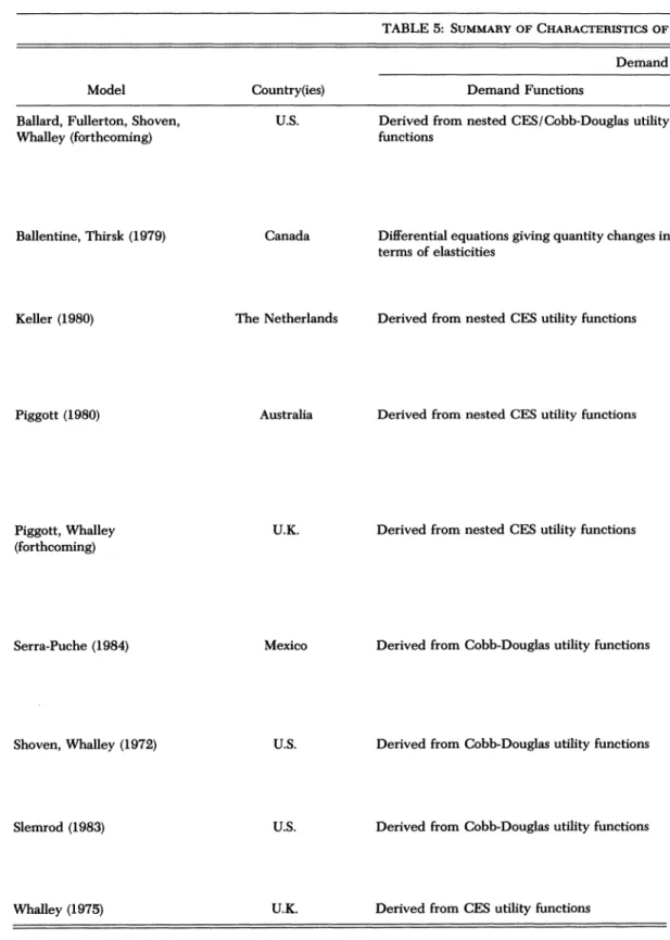
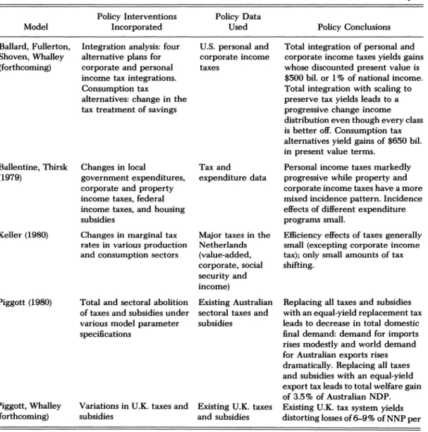
Later in the paper we describe models constructed to analyze alternative tax and trade policies in a number of countries.
The differences between these models and the numerical example above lie in their dimensionality (i.e., in the number of sectors modeled), their parameter spec- ification procedures which are based on empirical estimates, and their inclusion of more complex policy regimes than a sim- ple tax on one factor in one sector. The tax models vary in the degree to which they model the whole tax system; some attempt to incorporate the entire tax structure, while others include only those portions of the tax system relevant to the issues being directly examined. In the trade models, a key difference is between those models that are multicountry or global in orientation, and those that exam- ine how trade with the rest of the world affects individual countries.
Applied general-equilibrium analyses, then, are attempts to assemble and use models for policy evaluation. In the tax models, for instance, a proposal may be for the corporate tax to be abolished and replaced by a value-added tax. In trade models, multilateral tariff cuts proposed in a set of international negotiations could be the issue. Using applied general-equi- librium techniques, it is possible to com- pute alternative equilibria for different
policy regimes and to assess impacts of the change.
One point frequently made is that this approach would not be particularly in- structive if the equilibrium solution in any of these models were not unique for any particular tax or tariff policy. Uniqueness, or the lack of it, has been a long-standing interest of general-equilibrium theorists (Timothy Kehoe 1980). There is, however, no theoretical argument that guarantees uniqueness in the applied models de- scribed later. With some of the models, researchers have conducted ad hoc nu- merical experimentation (approaching equilibria from different directions and at different speeds), but have yet to find a case of nonuniqueness. In the case of the tax model of the U.S. due to Ballard, Don Fullerton, Shoven and Whalley (forthcom- ing), uniqueness has been numerically demonstrated by Kehoe and Whalley (1982). The current working hypothesis adopted by most modelers seems to be that uniqueness can be presumed for all of the models discussed here until a clear case of nonuniqueness is found.
Many other problems beyond the possi- bility of nonuniqueness are also encoun- tered in designing and using these models.
What type of model is to be used? Should it, for instance, be a traditional fixed-factor static model, or should it have dynamic features? Once the model form is deter- mined, how are functions and parameter values to be chosen? How are foreign trade, investment, government expendi- tures, and a range of other complicating features to be treated? How is the model to be solved? And, finally, even after the model has been solved, how are equilibria to be compared; that is, which summary statistics are to be used in evaluating the policy change? These questions apply equally to all applied general-equilibrium modeling efforts whether or not they are directed towards tax and trade-policy evaluation. We therefore now turn to a
1016 Journal of Economic Literature, Vol. XXII (September 1984) discussion of how these issues are dealt
with in the design of applied models.
III. Implementing Applied General- Equilibrium Analysis
A. Choosing the Model
Although the appropriate general- equilibrium model for tax or trade policy analysis depends partly on the focus of the model, most models currently in use have a similar form. They are variants of static, two-factor models that have long been employed in public finance and interna- tional trade, and are associated with the work of Eli Heckscher, Bertil Ohlin, Paul Samuelson, James Meade, Harry Johnson, and Arnold Harberger. Most computa- tional models involve more than two goods, while aggregating the factors of production into two broad types, capital and labor. In some models, these compos- ite factors are disaggregated into sub- groups (e.g., labor, distinguished by skilled and nonskilled). Intermediate transactions are also usually incorporated, either through fixed or flexible coefficient input- output matrices.
Perhaps a natural question is: Why have most models evolved in this way, when it is possible to use more general specifica- tions, possibly involving joint production2 and more alternative inputs than capital and labor composite factors? Although it is possible that in future work these fea- tures will gradually appear, at the present three reasons seem to account for the pop- ularity of basic two-factor structure in ap- plied work.
First, many policy issues have already been analyzed theoretically using this framework. If the major contribution of numerical work is to advance from quali- tative to quantitative analysis, it is clearly
natural to retain the same basic theoreti- cal structures. This way researchers can use the intuition gleaned from theoretical work to guide numerical investigations of policy alternatives.
Second, most data on which the numeri- cal specifications are based come in a form consistent with two-factor models. For in- stance, national accounts data identify wages and salaries and operating surpluses as major cost components. This suggests a model with capital and labor as inputs.
Input-output data provide intermediate transaction data, with value added broken down in a similar way.
Finally, the partition between goods and factors can be used in applied models so as to simplify computation and sharply reduce the costs of repeated solution. This is done by using factor prices to generate cost-covering goods prices, calculating consumer demands and evaluating the de- rived demands for factors (i.e., those amounts needed to meet consumer de- mands). In this way, even a model with large numbers of goods can be solved by working with a system of excess factor de- mands only. This simplification not only reduces execution costs for solution of models, but also makes feasible the incor- poration of more detail in the treatment of households and goods.
In some cases, static equilibrium models have been sequenced through time to re- flect changes in an economy's capital stock due to net saving. These models have been used to analyze intertemporal issues in tax policy, such as whether a move from an income tax to a consumption tax (under which saving is less heavily taxed) is desira- ble. Under this approach, a series of single- period equilibria are linked through sav- ing decisions that change the capital stock of the economy through time. Saving de- pends on the expected future return to assets acquired in the current period, with myopic expectations (i.e., expected future returns on assets equal current returns)
2The ORANI model (Peter Dixon, Brian Parmen- ter, John Sutton and D. Vincent 1982) incorporates joint production with empirically estimated transfor- mation frontiers.
frequently assumed to simplify computa- tions. At any point in time the economy has a stock of capital and a labor endow- ment; saving today augments the capital stock in all future periods. In each period a general equilibrium is computed in which all markets clear, including that for newly-produced capital goods. The econ- omy thus passes through a sequence of single-period equilibria that change through time as the capital stock grows.
A tax policy that encourages higher saving will also cause lowered consumption in the initial years, with an eventual higher consumption level due to the larger capi- tal stock.
A further issue in choosing one's model concerns the treatment of external sector transactions. In the multicountry trade models, a common approach is to use the so-called "Armington" formulation, which treats similar products produced in differ- ent countries as different goods. This dif- fers from theoretical Heckscher-Ohlin models in which it is assumed that prod- ucts are homogeneous across countries.
Among other reasons, the Armington for- mulation is usually adopted in order to accommodate the phenomenon of coun- tries both importing and exporting the same good (cross hauling). The external sector specification is also important in the tax models, since the effects of tax policies on an economy which is a taker of rental rates on world capital markets will be sig- nificantly different from those for a closed economy. Although international capital mobility is usually ignored, Lawrence Goulder, Shoven and Whalley (1983) have shown how its incorporation can change the analysis of tax policy options quite sub- stantially compared to a model with im- mobile capital.
Other issues in model design include the treatment of investment and govern- ment expenditures. Investment usu- ally reflects household-saving decisions (broadly defined to include corporate re-
tentions), which are based either on con- stant expenditure shares in static models or on intertemporal utility maximization in dynamic formulations. Government ex- penditures are usually broken down into transfers and real expenditures. The latter are frequently determined from utility- maximizing behavior for government: i.e., the government is treated as a separate consuming agent that buys public goods and services. In a few cases, models have been used with public goods in household utility functions, although this complicates the tax models.
B. Choosing Functional Forms
The major constraints on the selection of demand and production functions in all the applied models is that they be both consistent with the theoretical approach and analytically tractable. The first con- straint involves choosing functions that satisfy the restrictions listed in the presen- tation of general-equilibrium models, above, such as Walras' Law for demand functions. The second requires that the demand and supply responses of the econ- omy be reasonably easy to evaluate for any price vector considered as a candidate equilibrium solution for the economy.
This largely explains why the functional forms used are so often restricted to the family of "convenient" forms (Cobb- Douglas, Constant Elasticity of Substitu- tion (CES), Linear Expenditure System (LES), Constant Ratios of Elasticities of Substitution, Homothetic, (CRESH) Translog, and others).
The choice of a specific functional form typically depends on how elasticities are to be used in the model. This point is best illustrated by considering the demand side of these models. Demands derived from Cobb-Douglas utility functions are easy to work with, but have the restric- tions of unitary income and uncompen- sated own-price elasticities, and zero cross-price elasticities. These restrictions
1018 Journal of Economic Literature, Vol. XXII (September 1984) are typically implausible, given empirical
estimates of elasticities applicable to any particular model, but can only be relaxed by using more general functional forms.
With CES functions, unitary own-price elasticities no longer apply. However, if all expenditure shares are small, the com- pensated own-price elasticities equal the elasticity of substitution in the prefer- ences, and it may be unacceptable to model all commodities as having essen- tially the same compensated own-price elasticities. A response to this difficulty is to use hierarchical or nested CES func- tions, adding further complexity in struc- ture. The unitary income elasticity feature of the Cobb-Douglas functions can also be relaxed. One way is to use LES functions with a displaced origin, but then the origin displacements need to be specified. The general approach seems to be one of se- lecting the functional form that best al- lows key parameter values (e.g., income and price elasticities) to be incorporated, while retaining tractability.
On the production side, CES value- added functions are usually used to allow for substitution between primary factors.
If more than two factors are used, hierar- chical CES functions are again used. The intermediate production functions are sometimes modeled as fixed coefficients;
on other occasions, some intermediate substitutability is allowed. In the interna- tional trade model one specification used is to have fixed coefficients in terms of composite goods, but with substitution possible among the components of the composite. By way of example, a fixed steel requirement per car may be speci- fied, but with substitution between im- ported and domestic steel represented by CES functions. This may be necessary be- cause of the large amount of trade in inter- mediate products and the unrealistically low import price elasticities that fixed coefficient intermediate production would imply if the Armington treatment
of differentiating products by country is used.
C. Selecting Parameter Values
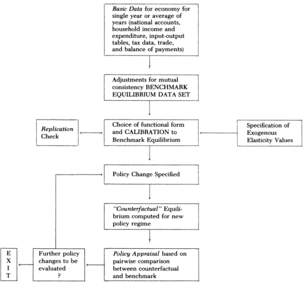
Parameter values for the functional forms are frequently crucial in determin- ing results of policy simulations generated by the applied models. The procedure most commonly used to select parameter values has come to be labeled "cali- bration" (Ahsan Mansur and Whalley 1984). This procedure is outlined in Fig- ure 1. The economy under consideration is assumed to be in equilibrium, a so-called
"benchmark" equilibrium. The parame- ters of the model are chosen such that the model can reproduce this data set as an equilibrium solution.3 If CES or LES func- tions are used in the model, exogenously specified elasticity values (usually based on literature estimates) are also required in this procedure because the benchmark data only give price and quantity observa- tions associated with a single equilibrium.
On the demand side, for instance, only the slope of the budget constraints at the equilibrium consumption quantities is given by the benchmark data. The param- eter values thus generated can then be used to solve for the alternative equilib- rium associated with any changed policy regime. These are usually termed "coun- terfactual" or "policy replacement" equi- libria.
In practice, benchmark equilibria are constructed from national accounts and other government data sources. In gen- eral, the information will be inconsistent (e.g., payments to labor from firms will not equal labor income received by house-
3An additional important feature of this procedure is that once calibration is complete, it should be possi- ble to reproduce the benchmark equilibrium data set as an equilibrium solution of the model. This is the replication check referred to in Figure 1, which serves as an important accuracy test of a computer code. If the replication check fails, then a program- ming error has been discovered and the coding must be investigated further.
Basic Data for economy for single year or average of years (national accounts, household income and expenditure, input-output tables, tax data, trade, and balance of payments)
Adjustments for mutual consistency BENCHMARK EQUILIBRIUM DATA SET
Replication Choice of functional form Specification of Check
ai
-* and CALIBRATION to Exogenous
Benchmark Equilibrium Elasticity Values
Policy Change Specified
"Counterfactual" Equili- brium computed for new policy regime
E Further policy Policy Appraisal based on X changes to be pairwise comparison
I evaluated between counterfactual
T ? and benchmark
Figure 1. Flow chart outlining calibration procedures and model use in typical applied general- equilibrium model
holds), and a number of adjustments are required to the basic data to ensure that equilibrium conditions hold. Some data are taken as correct and others are ad- justed to be consistent in the process of generating a benchmark data set. The construction of data sets of this type is de- scribed in Kemal Dervis, Jaime de Melo and Sherman Robinson (1982), France St.
Hilaire and Whalley (1983), John Piggott and Whalley (forthcoming), and Ballard, Fullerton, Shoven and Whalley (forthcom- ing). Because the benchmark data are usu-
ally produced in value terms, units must be chosen for goods and factors so that separate price and quantity observations are obtained. A commonly used units con- vention, originally adopted by Harberger, is to choose units for both goods and fac- tors so that they have a price of unity in the benchmark equilibrium.
Typically, calibration involves only one year's data, or a single observation repre- sented as an average over a number of years. A crucial point in using calibration is that because of the reliance on a single