Globalization of business operations and diversification of the market require firms to

Abstract

Globalization of business operations and diversification of the market require firms to

organize flexible and effective supply systems. Supply chain management (SCM) is well

known as a strategic management approach to optimize the business process. In this

paper, we consider a supply chain consisting of a single manufacturer and a number of

suppliers. We suppose that the manufacturer decides buying prices of suppliers’ products

and purchase allocation to the suppliers, while suppliers compete on the frequency of

delivery to the manufacturer. The purpose of this paper is to determine optimal buying

prices, delivery frequencies and demand allocations that minimize the total cost incurred

by the manufacturer and maximize the profit made by the suppliers. We first establish a

mathematical model of decision-making in the supply chain as a tri-level non-cooperative

game. We then formulate the game as an optimization problem to obtain optimal

strategies and provide a numerical method with a smoothing technique. Moreover, we

conduct numerical experiments and discuss the property and behavior of solutions.

Contents

1 Introduction 1

2 Preliminaries 2

2.1 Nash equilibria and stationary Nash equilibria . . . . 2 2.2 Smoothing technique for complementarity conditions . . . . 3

3 A mathematical model of a supply chain 3

4 Formulations 5

4.1 Manufacturer’s optimization problem for demand allocations . . . . 6 4.2 Suppliers’ NEP for delivery frequencies . . . . 7 4.3 Manufacturer’s optimization problem for buying prices . . . . 9

5 Numerical experiments 10

6 Conclusion 16

1 Introduction

Now that business operations are globalized and the market is diversified, constructing a supply system which is able to respond quickly to the demand is an important issue for many firms. Supply chain management (SCM) is well known as a strategic man- agement approach to optimize the business process, and a number of firms including manufacturing enterprises are managed under SCM. Supply chain is a supply system of products that involves the procurement of materials, production, delivery, and sale [16]. In general, each process in a supply chain is managed individually and there are multiple decision makers in a supply chain. Therefore, it is important for SCM to clar- ify the decision-making process and optimize it from a broad perspective. In particular, controlling the balance of Purchase-Sales-Inventory (PSI) is thought to be a key to SCM, and how to optimize PSI has been discussed from various points of view [1, 9].

In this paper, we focus on pricing and delivery strategies related to PSI on SCM. We consider a contract between a number of suppliers and a single manufacturer, where suppliers engage in production and delivery of products, while the manufacturer makes use of suppliers’ products with holding them as inventories. The manufacturer orders and buys products from suppliers so as to meet the demand. Here, we suppose that the manufacturer decides buying prices of suppliers’ products and purchase allocation to the suppliers, while suppliers compete on the frequency of delivery to the manufacturer. The main purpose of this paper is to determine optimal buying prices, delivery frequencies and demand allocations that minimize the total cost incurred by the manufacturer and maximize the profit made by each supplier. To obtain the optimal solution, we firstly establish a mathematical model of decision-making in a supply chain composed of one manufacturer and n suppliers as a tri-level non-cooperative game. Then, based on this model, we formulate an optimization problem for determining the optimal strategies.

The steps of the formulation are as follows. We begin with the manufacturer’s optimiza- tion problem for demand allocation. Next, we consider the suppliers’ Nash equilibrium problem for delivery frequency. In the end, we finish with the manufacturer’s optimiza- tion problem for buying prices.

The rest of this paper is organized as follows. Section 2 gives the definition of equilibria in a Nash game and describes a smoothing technique to transform complementarity conditions into differentiable equations approximately, as preliminaries to the subsequent sections. Section 3 establishes a mathematical model of the supply chain we consider.

Section 4 formulates the optimization problem we have to solve. Section 5 investigates

the property and behavior of the solution by numerical experiments on a simple example

of the supply chain. Section 6 concludes the paper.

2 Preliminaries

In this section, we explain Nash games with the definition of equilibria and a smoothing technique to transform complementarity conditions into differentiable equations approx- imately.

2.1 Nash equilibria and stationary Nash equilibria

Here we state the Nash equilibrium problem (NEP) and provide the definitions of Nash equilibria and stationary Nash equilibria.

In the classical Nash game, all players choose their own strategies simultaneously under their respective constraints and try to minimize their own objective functions noncooperatively [13, 14]. NEP is a problem of seeking a tuple of strategies resulting from the game. The problems solved by each player in the Nash game are formulated as the following optimization problems [5, 6, 10, 11, 15]:

min x

θ ν (x ν , x ₋ ν ) s.t. x _ν ∈ X _ν

 

 (ν = 1, . . . , N ), (1)

where N is the number of players and x ∈ R ⁿ denotes a strategy vector composed of all players’ strategies x ν ∈ R ⁿ

, ν = 1, . . . , N , where n = ∑ _N

ν=1 n ν . For ν = 1, . . . , N , a tuple of all players’ strategies except that of player ν is denoted by x _{− ν} , and player ν’s objective function and strategy set are denoted by θ ν and X ν , respectively. Note that we write θ _ν (x) = θ _ν (x _ν , x _{− ν} ) to emphasize the role of x _ν in this problem.

A tuple of strategies x ^∗ = (x ^∗ ₁ , . . . , x ^∗ _N ) ^T is called a Nash equilibrium if for all ν = 1, . . . , N,

θ ν (x ^∗ _ν , x ^∗ _{− ν} ) ≤ θ ν (x ν , x ^∗ _{− ν} ), ∀ x ν ∈ X ν .

In short, Nash equilibrium is a tuple of strategies such that no player can benefit by changing his/her own strategy unilaterally.

On the other hand, a tuple of strategies x ^∗ is called a stationary Nash equilibrium if, for all ν = 1, . . . , N , x ^∗ _ν is a stationary point for the optimization problem (1) with x ₋ ν = x ^∗ _{− ν} , where a stationary point means that it satisfies a first-order optimality condition for the problem [11]. For example, in the case that the strategy set of player ν is given by the inequality constraint g ν (x ν ) ≤ 0 for each ν, where g ν : R ⁿ

→ R ^m

for some m _ν , a stationary Nash equilibrium x ^∗ along with Lagrange multipliers γ = (γ ₁ , . . . , γ _N ) ^T satisfies the following Karush-Kuhn-Tucker (KKT) system [2]:

∇ x

θ ν (x ν , x ₋ ν ) + ∇ x

g ν (x ν ) ^T γ ν = 0 (ν = 1, . . . , N ),

γ _ν ≥ 0, g _ν (x _ν ) ≤ 0, γ _ν ^T g _ν (x _ν ) = 0 (ν = 1, . . . , N).

Note that if problems (1) are convex, then the concept of stationary Nash equilibrium reduces to that of Nash equilibrium.

2.2 Smoothing technique for complementarity conditions

Here we describe a technique to transform complementarity conditions into differen- tiable equations approximately.

The complementarity condition a ≥ 0, b ≥ 0, ab = 0, a, b ∈ R can be written equiv- alently as the equation ϕ _{F B} (a, b) = 0, where ϕ _{F B} : R ² → R is the Fischer-Burmeister (FB) function [7, 12] defined by ϕ _{F B} (a, b) = a + b − √

a ² + b ² . This is because the FB function has the following property:

ϕ _{F B} (a, b) = 0 ⇔ a ≥ 0, b ≥ 0, ab = 0.

However, the equation ϕ F B (a, b) = 0 is not always easy to deal with, since the FB function ϕ _{F B} (a, b) is not differentiable at (a, b) = (0, 0). To circumvent this difficulty, we introduce the smoothing Fischer-Burmeister (SFB) function defined by ϕ ^µ _{F B} (a, b) = a+b − √

a ² + b ² + 2µ ² with a parameter µ > 0, and replace the equation ϕ _{F B} (a, b) = 0 by the equation ϕ ^µ _{F B} (a, b) = 0. For any fixed µ > 0, the SFB function ϕ ^µ _{F B} is continuously differentiable everywhere and has the following property:

ϕ ^µ _{F B} (a, b) = 0 ⇔ a > 0, b > 0, ab = µ ² .

Furthermore, ϕ ^µ _{F B} (a, b) coincides with ϕ F B (a, b) if µ = 0, and ϕ ^µ _{F B} (a, b) ≈ ϕ F B (a, b) if µ > 0 is sufficiently small. The fundamental idea underlying a smoothing technique is to approximate the complementarity condition a ≥ 0, b ≥ 0, ab = 0 by such a smooth equation [3, 4, 8, 11].

3 A mathematical model of a supply chain

In this section, we describe a mathematical model of the supply chain treated in this paper.

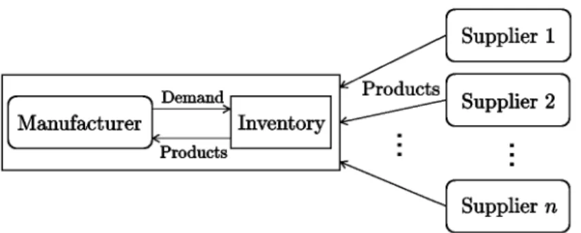
We consider a supply chain consisting of one manufacturer and n suppliers, where

suppliers engage in production and delivery of products, while the manufacturer makes

use of suppliers’ products with holding them as inventories (see Figure 1). The suppliers

incur production, shipment and transportation costs of products, and the manufacturer

bears inventory holding costs. In this supply chain, we suppose that the manufacturer

decides buying prices of suppliers’ products and purchase allocation to the suppliers so

as to minimize the total cost, while each supplier determines the frequency of delivery

to the manufacturer so as to maximize the profit.

Figure 1: Supply chain model

In this paper, we regard this decision-making process as a tri-level non-cooperative game between the manufacturer and suppliers. At the upper level, the manufacturer presents buying prices to the suppliers. At the middle level, the suppliers compete on the frequency of delivery to the manufacturer in response to the buying prices given by the manufacturer. At the lower level, the manufacturer determines the demand allocations to the suppliers in response to the suppliers’ delivery frequencies that form a Nash equilibrium in a non-cooperative game by the suppliers.

First, we list the symbols that represent the parameters and variables used to model the supply chain.

Parameters

D (> 0): the expected demand of the manufacturer h (> 0): unit inventory holding cost of the manufacturer

l i (> 0): lower bound of the expected delivery frequency of supplier i u i ( ≥ l i ): upper bound of the expected delivery frequency of supplier i

c i (> 0): unit cost of production of supplier i k _i (> 0): unit cost of delivery of supplier i K _i (> 0): fixed cost of delivery of supplier i

q _i (> 0): unit profit to be guaranteed by the product of supplier i Variables

p i (≥ c i + k i + q i ): unit buying price of the product, determined by the manufacturer r i (l i ≤ r i ≤ u i ): supplier i’s expected delivery frequency, determined by supplier i

λ i (0 ≤ λ i ≤ 1): demand allocation to each supplier i, determined by the manufacturer

For simplicity of discussion, we regard the demand D as a deterministic parameter.

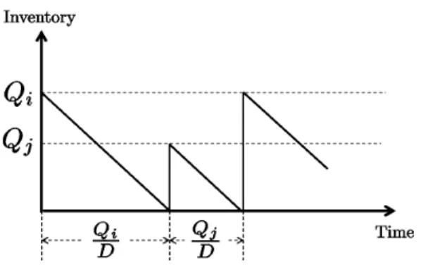
Furthermore we assume that suppliers can produce and deliver the products at once,

Figure 2: An example of inventory transition

and we do not take into consideration the time each supplier requires to produce, ship and transport the products. Moreover, we suppose that each supplier produces and delivers the products when the manufacturer’s inventory gets empty and that two or more suppliers do not deliver the products simultaneously. Let Q i denote the quantity of the products per delivery for each supplier i. Then it is written as Q _i = λ _i D/r _i by the definition of parameters and variables. Under the above assumptions, an example of inventory transition can be depicted as in Figure 2.

4 Formulations

In this section, we formulate a problem for determining optimal strategies in the supply chain model established in the previous section.

We begin with the total cost incurred by the manufacturer and the profit made by each supplier. Let I i denote the total quantity of inventories resulting from supplier i’s deliveries in a unit period. Then, by the EOQ logic, it can be expressed as

I i = r i Q ² _i

2D = λ ² _i D 2r _i .

From this and the fact that the total cost incurred by the manufacturer is the sum of purchasing costs and inventory holding costs, the cost function of the manufacturer, denoted by C(p, r, λ), can be written as follows:

C(p, r, λ) =

∑ n i=1

(p _i λ _i D + hI _i ) =

∑ n i=1

(

p _i λ _i D + h λ ² _i D 2r i

)

, (2)

where p = (p ₁ , . . . , p _n ) ^T , r = (r ₁ , . . . , r _n ) ^T and λ = (λ ₁ , . . . , λ _n ) ^T .

On the other hand, the profit made by each supplier is selling benefits minus shipping costs. Thus, the profit function of each supplier i, denoted by Φ _i (p, r, λ), can be written as follows:

Φ _i (p, r, λ) = (p _i − c _i − k _i ) λ _i D − r _i K _i (i = 1, . . . , n). (3)

Using these functions, we formulate the problems that constitute the three-stage model, by the following steps. First, for any fixed buying price p and delivery fre- quency r, we formulate an optimization problem for demand allocation λ to obtain the optimal demand allocations of the manufacturer. Next, for any fixed buying price p, we consider a NEP for delivery frequency r to derive the equilibrium delivery frequencies of the suppliers. Last, we formulate an optimization problem for buying price p to obtain the optimal buying prices of the manufacturer.

4.1 Manufacturer’s optimization problem for demand allocations We describe the manufacturer’s problem for determining an optimal demand allocation λ for any fixed buying price p and delivery frequency r. The optimal demand allocation for given p and r can be regarded as a function of p and r. So we denote it as λ ^∗ (p, r) = (λ ^∗ ₁ (p, r), . . . , λ ^∗ _n (p, r)) ^T .

The demand allocations of the manufacturer must satisfy the conditions that each allocation is nonnegative and the sum of all allocations is equal to 1. Therefore, the problem to obtain λ ^∗ (p, r) is formulated as the following optimization problem:

min λ C(p, r, λ) s.t.

∑ n i=1

λ _i = 1,

λ i ≥ 0 (i = 1, . . . , n).

(4)

By the definition (2), the objective function C(p, r, λ) is strictly convex and quadratic in λ. Thus the optimal solution of problem (4) exists and is unique. In addition, it is necessary and sufficient that the optimal solution along with Lagrange multipliers v and w = (w 1 , . . . , w n ) ^T satisfies the following KKT conditions:

(

p _i + ^hλ _r

i

)

D − v − w _i = 0 (i = 1, . . . , n), 0 ≤ w i ⊥ λ i ≥ 0 (i = 1, . . . , n),

1 − ∑ ⁿ

i=1

λ _i = 0,

(5)

where a ⊥ b means ab = 0.

By substituting the first equation of (5) into the second one, we have 0 ≤

(

p i + hλ i

r _i )

D − v ⊥ λ i ≥ 0 (i = 1, . . . , n).

Using the SFB function, the KKT conditions (5) can be approximated by the following

system of differentiable equations:

ϕ ^µ _{F B} ((p _i + h ^λ _r

i

)D − v, λ _i ) = 0 (i = 1, . . . , n), 1 − ∑ ⁿ

i=1

λ i = 0.

(6)

We write Lagrange multiplier v which along with λ ^∗ (p, r) satisfies the KKT conditions (5) as v ^∗ (p, r). It follows from the property of the SFB function that a solution of the equation system (6) for a sufficiently small smoothing parameter µ > 0 can be seen as an approximation of λ ^∗ (p, r) and v ^∗ (p, r).

4.2 Suppliers’ NEP for delivery frequencies

We describe the suppliers’ Nash game in which each supplier i optimizes delivery frequency r i for any fixed buying price p. The equilibrium delivery frequency for a given p can be regarded as a function of p. So we denote it as r ^∗ (p) = (r ₁ ^∗ (p), . . . , r _n ^∗ (p)) ^T . In the supply chain under consideration, the optimization problems the suppliers are to solve can be formulated as follows.

The delivery frequency of each supplier i has lower and upper bounds given by l i

and u _i , respectively. From these constraints and the fact that the optimal solution of problem (4) is λ ^∗ (p, r), the suppliers solve the following problems:

max r

Φ _i (p, r, λ ^∗ (p, r)) s.t. l i ≤ r i ≤ u i

 

 (i = 1, . . . , n). (7) The equilibrium delivery frequency r ^∗ (p) is the solution of a NEP consisting of the optimization problems (7).

Since a pair of λ ^∗ (p, r) and v ^∗ (p, r) is the solution of the KKT conditions (5) which can be approximated by the equation system (6), problems (7) are approximately rewritten as the following problems:

r max

,λ,v Φ _i (p, r, λ) s.t. l i ≤ r i ≤ u i ,

ϕ ^µ _{F B} ((p _j +

)D − v, λ _j ) = 0 (j = 1, . . . , n), 1 − ∑ ⁿ

j=1

λ j = 0

 

 

 

 

 



 

 

 

 

 

(i = 1, . . . , n). (8)

By the definition (3), the objective function Φ _i (p, r, λ) is concave in r _i , λ and v, but the

feasible set of each player i’s problem is not convex. So, it is difficult to deal with the

Nash equilibrium in the game consisting of problems (8). To circumvent this difficulty, we replace the Nash equilibrium with the stationary Nash equilibrium.

The stationary Nash equilibrium in the game composed of problems (8), along with Lagrange multipliers ζ = (ζ ₁ , . . . , ζ _n ) ^T , η = (η ₁ , . . . , η _n ) ^T , ξ ₁ = (ξ ₁₁ , . . . , ξ _1n ) ^T , . . . , ξ _n = (ξ n1 , . . . , ξ nn ) ^T , ν = (ν 1 , . . . , ν n ) ^T , satisfies the following KKT system:

K i − ζ i + η i + ξ ii ∇ r

ϕ ^µ _{F B} ((p i +

)D − v, λ i ) = 0, ξ _ij ∇ λ

ϕ ^µ _{F B} ((p _j +

)D − v, λ _j ) − ν _i = 0

(j = 1, . . . , n, j ̸ = i),

− (p i − c i − k i )D + ξ ii ∇ λ

ϕ ^µ _{F B} ((p i +

)D − v, λ i ) − ν i = 0,

∑ n j=1

ξ _ij ∇ v ϕ ^µ _{F B} ((p _j +

)D − v, λ _j ) = 0, 0 ≤ ζ _i ⊥ r _i − l _i ≥ 0,

0 ≤ η i ⊥ u i − r i ≥ 0,

ϕ ^µ _{F B} ((p i +

)D − v, λ i ) = 0

 

 

 

 

 

 

 

 

 

 

 

 

 

 

 

 

 

 

 

 

 

 

 



(i = 1, . . . , n),

1 − ∑ ⁿ

i=1

λ _i = 0.

(9)

Again, by applying the SFB function to the complementarity conditions 0 ≤ ζ _i ⊥ r _i − l _i ≥ 0 (i = 1, . . . , n),

0 ≤ η i ⊥ u i − r i ≥ 0 (i = 1, . . . , n),

the KKT system (9) can be approximated by the following system of smooth equations:

K _i − ζ _i + η _i + ξ _ii ∇ r

ϕ ^µ _{F B} ((p _i +

)D − v, λ _i ) = 0, ξ ij ∇ λ

ϕ ^µ _{F B} ((p j +

)D − v, λ j ) − ν i = 0

(j = 1, . . . , n, j ̸= i),

− (p _i − c _i − k _i )D + ξ _ii ∇ λ

ϕ ^µ _{F B} ((p _i +

)D − v, λ _i ) − ν _i = 0,

∑ n j=1

ξ _ij ∇ v ϕ ^µ _{F B} ((p _j +

)D − v, λ _j ) = 0, ϕ ^µ _{F B} (ζ i , r i − l i ) = 0,

ϕ ^µ _{F B} (η _i , u _i − r _i ) = 0,

ϕ ^µ _{F B} ((p i +

)D − v, λ i ) = 0

 

 

 

 

 

 

 

 

 

 

 

 

 

 

 

 

 

 

 

 

 

 

 



(i = 1, . . . , n),

1 − ∑ ⁿ

i=1

λ i = 0.

(10)

We denote the solution r and the Lagrange multipliers ζ, η, ξ ₁ , . . . , ξ _n and ν that sat-

isfy the KKT system (9) as r ^∗ , ζ ^∗ (p) = (ζ ₁ ^∗ (p), . . . , ζ _n ^∗ (p)) ^T , η ^∗ (p) = (η ₁ ^∗ (p), . . . , η _n ^∗ (p)) ^T ,

ξ ^∗ ₁ (p) = (ξ ₁₁ ^∗ (p), . . . , ξ _1n ^∗ (p)) ^T , . . . , ξ ^∗ _n (p) = (ξ _n1 ^∗ (p), . . . , ξ _nn ^∗ (p)) ^T and ν ^∗ (p) = (ν ₁ ^∗ (p), . . . , ν _n ^∗ (p)) ^T . From the property of the SFB function, a solution of the equation system (10) for a sufficiently small smoothing parameter µ > 0 can be regarded as an approximation of r ^∗ (p), ζ ^∗ (p), η ^∗ (p), ξ ^∗ ₁ (p), . . . , ξ ^∗ _n (p) and ν ^∗ (p).

4.3 Manufacturer’s optimization problem for buying prices

Finally, we state the manufacturer’s problem to optimize the buying price p. We denote the optimal buying price as p ^∗ = (p ^∗ ₁ , . . . , p ^∗ _n ) ^T .

The buying price of each supplier i’s products has the lower bound c _i + k _i + q _i . More- over, because of the fact that the optimal solution of problem (4) is λ ^∗ (p, r) and the stationary Nash equilibrium in the game composed of problems (7) is r ^∗ (p), the manufac- turer’s problem of determining p ^∗ is formulated as the following optimization problem:

min p C(p, r ^∗ (p), λ ^∗ (p, r ^∗ (p))) s.t. p i ≥ c i + k i + q i (i = 1, . . . , n).

(11)

From the discussion above, we find that a pair of λ ^∗ (p, r) and v ^∗ (p, r) can be ap- proximated by a solution of the equation system (6), and a solution of the equation system (10) yields an approximation of a tuple of r ^∗ (p), ζ ^∗ (p), η ^∗ (p), ξ ^∗ ₁ (p), . . . , ξ ^∗ _n (p) and ν ^∗ (p). Consequently, problem (11) is approximately reformulated as the following problem:

p,r,λ,v,ζ,η,ξ min

,...,ξ

,ν C(p, r, λ)

s.t. K i − ζ i + η i + ξ ii ∇ r

ϕ ^µ _{F B} ((p i +

)D − v, λ i ) = 0, ξ _ij ∇ λ

ϕ ^µ _{F B} ((p _j +

)D − v, λ _j ) − ν _i = 0

(j = 1, . . . , n, j ̸ = i),

−(p i − c i − k i )D + ξ ii ∇ λ

ϕ ^µ _{F B} ((p i +

)D − v, λ i ) − ν i = 0,

∑ n j=1

ξ ij ∇ v ϕ ^µ _{F B} ((p j +

)D − v, λ j ) = 0, ϕ ^µ _{F B} (ζ _i , r _i − l _i ) = 0,

ϕ ^µ _{F B} (η i , u i − r i ) = 0,

ϕ ^µ _{F B} ((p _i +

)D − v, λ _i ) = 0

 

 

 

 

 

 

 

 

 

 

 

 

 

 

 

 

 

 

 

 

 

 

 



(i = 1, . . . , n),

1 − ∑ ⁿ

i=1

λ _i = 0.

(12)

In summary, the optimal buying price p ^∗ , the equilibrium delivery frequency r(p ^∗ ) and the optimal demand allocation λ ^∗ (p ^∗ , r ^∗ (p ^∗ )) can be obtained by finding an optimal solution of problem (12) for a sufficiently small smoothing parameter µ > 0.

5 Numerical experiments

In this section, we show some numerical results on a simple example of the supply chain. For the model formulated in the previous section, we consider a supply chain consisting of one manufacturer and two suppliers, that is, the case n = 2. Then we investigate the behavior of the solutions, the manufacturer’s total cost C, and the sup- pliers’ profits Φ 1 and Φ 2 for various values of the parameters. All computations were carried out on a machine with Intel(R)Core(TM)2Duo 3.00GHz CPU. We solved prob- lem (12) by the solver fmincon in MATLAB 2007a. We examined the following six cases with the upper and lower bounds of the suppliers’ delivery frequencies l ₁ = l ₂ = 0.1 and u 1 = u 2 = 2.0, respectively, and the guaranteed unit profit q 1 = q 2 = 0.1 in all cases.

Case1. Changing the unit inventory holding cost: Let h be increased from 0.5 to 3.5, with c ₁ = c ₂ = 0.1, k ₁ = k ₂ = 0.1 and K ₁ = K ₂ = 0.1.

Case2. Changing the expected demand: Let D be increased from 0.5 to 2.0, with c 1 = c 2 = 0.1, k 1 = k 2 = 0.1 and K 1 = K 2 = 0.1.

Case3. Changing the sum of unit production cost and unit delivery cost of both sup- pliers: Let c i + k i (i = 1, 2) be increased from 0.01 to 0.3, with h = 1.0, D = 1.0 and K ₁ = K ₂ = 0.1.

Case4. Changing the fixed delivery cost of both suppliers: Let K _i (i = 1, 2) be increased from 0.01 to 0.3, with h = 1.0, D = 1.0, c 1 = c 2 = 0.1 and k 1 = k 2 = 0.1.

Case5. Changing the sum of unit production cost and unit delivery cost of supplier 2:

Let c 1 + k 1 be fixed at 0.2 and c 2 +k 2 be increased from 0.2 to 0.5, with h = 1.0, D = 1.0 and K ₁ = K ₂ = 0.1.

Case6. Changing the fixed delivery cost of supplier 2: Let K ₁ be fixed at 0.1 and K ₂ be increased from 0.1 to 0.4, with h = 1.0, D = 1.0, c 1 = c 2 = 0.1 and k 1 = k 2 = 0.1.

The solutions, the manufacturer’s total costs, and the suppliers’ profits in Cases 1 – 4 are shown in Figure 3 – 6, respectively. The solutions in Case 5 and Case 6 are presented in Table 1 and Table 2, respectively. The manufacturer’s total costs and the suppliers’

profits in Case 5 and Case 6 are described in Figure 7 and Figure 8, respectively.

Figure 3: The optimal buying price p ^∗ = (p ^∗ ₁ , p ^∗ ₂ ), the equilibrium delivery frequency r ^∗ = (r ^∗ ₁ , r ^∗ ₂ ), the manufacturer’s total cost C, and the suppliers’ profits Φ ₁ and Φ ₂ , in Case 1

Figure 4: The optimal buying price p ^∗ = (p ^∗ ₁ , p ^∗ ₂ ), the equilibrium delivery frequency

r ^∗ = (r ^∗ ₁ , r ^∗ ₂ ), the manufacturer’s total cost C, and the suppliers’ profits Φ ₁ and Φ ₂ , in

Case 2

Figure 5: The optimal buying price p ^∗ = (p ^∗ ₁ , p ^∗ ₂ ), the equilibrium delivery frequency r ^∗ = (r ^∗ ₁ , r ^∗ ₂ ), the manufacturer’s total cost C, and the suppliers’ profits Φ ₁ and Φ ₂ , in Case 3

Figure 6: The optimal buying price p ^∗ = (p ^∗ ₁ , p ^∗ ₂ ), the equilibrium delivery frequency

r ^∗ = (r ^∗ ₁ , r ^∗ ₂ ), the manufacturer’s total cost C, and the suppliers’ profits Φ ₁ and Φ ₂ , in

Case 4

Table 1: The optimal buying price p ^∗ = (p ^∗ ₁ , p ^∗ ₂ ), the equilibrium delivery frequency r ^∗ = (r ₁ ^∗ , r ₂ ^∗ ), and the optimal demand allocation λ ^∗ = (λ ^∗ ₁ , λ ^∗ ₂ ), in Case 5

(c 1 + k 1 , c 2 + k 2 ) (0.2, 0.2) (0.2, 0.3) (0.2, 0.4) (0.2, 0.5)

p ^∗ ₁ 0.5162 0.5022 0.4919 0.4831

p ^∗ ₂ 0.5162 0.6363 0.7627 0.8892

r ^∗ ₁ 0.7906 0.8287 0.8557 0.8604

r ^∗ ₂ 0.7906 0.7452 0.6885 0.6156

λ ^∗ ₁ 0.5000 0.5791 0.6575 0.7287

λ ^∗ ₂ 0.5000 0.4209 0.3425 0.2713

Figure 7: The manufacturer’s total cost C and the suppliers’ profits Φ 1 and Φ 2 , in Case

5

Table 2: The optimal buying price p ^∗ = (p ^∗ ₁ , p ^∗ ₂ ), the equilibrium delivery frequency r ^∗ = (r ₁ ^∗ , r ₂ ^∗ ), and the optimal demand allocation λ ^∗ = (λ ^∗ ₁ , λ ^∗ ₂ ), in Case 6

(K 1 , K 2 ) (0.1, 0.1) (0.1, 0.2) (0.1, 0.3) (0.1, 0.4) p ^∗ ₁ 0.5162 0.5022 0.4973 0.4946 p ^∗ ₂ 0.5162 0.6747 0.7943 0.8902 r ^∗ ₁ 0.7906 0.7760 0.7155 0.6577 r ^∗ ₂ 0.7906 0.4870 0.3410 0.2586 λ ^∗ ₁ 0.5000 0.6660 0.7459 0.7912 λ ^∗ ₂ 0.5000 0.3340 0.2541 0.2088

Figure 8: The manufacturer’s total cost C and the suppliers’ profits Φ 1 and Φ 2 , in Case

6

In all cases, when the problem data are identical between the two suppliers, buying prices p ^∗ ₁ and p ^∗ ₂ , delivery frequencies r ₁ ^∗ and r ₂ ^∗ , and demand allocations λ ^∗ ₁ and λ ^∗ ₂ are all equal to each other, and the profits of both suppliers are also equal. Moreover, the supplier whose products are priced lower takes a higher delivery frequency and obtains a higher demand allocation in both Case 5 and Case 6.

In Case 1, as the unit holding cost h increases, buying prices p ^∗ ₁ and p ^∗ ₂ as well as delivery frequencies r 1 and r 2 also increase. Furthermore, the manufacturer’s total cost C increases, and both suppliers’ profits Φ ₁ and Φ ₂ also increase. As h increases, the inventory holding cost ∑ ₂

i=1 hλ ² _i /2r i tends to share a larger part of the total cost C.

This may suggest that the manufacturer increases p ₁ and p ₂ anticipating the reduction in inventory holding costs caused by the increase in r ₁ and r ₂ , and attempts to avoid a massive increase in the total cost C.

In Case 2, as the expected demand D increases, buying prices p ^∗ ₁ and p ^∗ ₂ decrease, and delivery frequencies r 1 and r 2 increase. Moreover, the manufacturer’s total cost C increases, and both suppliers’ profits Φ ₁ and Φ ₂ also increase. As D increases, the selling benefits (p i − c i − k i )λ i D (i = 1, 2) tend to hold a larger part of the profits Φ _i (i = 1, 2). Thus we may expect that the suppliers increase delivery frequencies r ₁ and r 2 to obtain higher demand allocations for selling benefits. This suggests that the manufacturer increases p ₁ and p ₂ to prevent the total cost C from increasing greatly.

In Case 3, as the sums of unit production cost and unit delivery cost of both suppliers c _i + k _i (i = 1, 2) increase, buying prices p ^∗ ₁ and p ^∗ ₂ increase, but delivery frequencies r ₁ and r 2 do not change. In addition, the manufacturer’s total cost C increases, and both suppliers’ profits Φ ₁ and Φ ₂ do not change. As c _i + k _i (i = 1, 2) increase, the selling benefits (p i − c i − k i )λ i D (i = 1, 2) become less in the profits Φ i (i = 1, 2). This may reflect the fact that the manufacturer increases p ₁ and p ₂ worrying about a massive increase in the total cost C caused by the decrease in r 1 and r 2 .

In Case 4, as the fixed delivery costs of both suppliers K _i (i = 1, 2) increase, buying prices p ^∗ ₁ and p ^∗ ₂ increase, and delivery frequencies r 1 and r 2 decrease. Moreover, the manufacturer’s total cost C increases, and both suppliers’ profits Φ ₁ and Φ ₂ also increase.

As K 1 and K 2 increase, the shipping costs r i K i (i = 1, 2) tend to occupy a larger part of the profits Φ _i (i = 1, 2). We may expect that the suppliers decrease delivery frequencies r 1 and r 2 to cut down the shipping costs. This suggests that the manufacturer increases p ₁ and p ₂ to prevent the total cost C from increasing largely.

In Case 5, as the sum of unit production cost and unit delivery cost c 2 + k 2 of sup- plier 2 increases, buying price p ^∗ ₁ decreases but p ^∗ ₂ increases, and delivery frequency r 1

increases but r ₂ decreases. Furthermore, demand allocation λ ₁ increases, λ ₂ decreases,

the manufacturer’s total cost C and supplier 1’s profit Φ 1 increase, and supplier 2’s profit

Φ ₂ decreases. As c ₂ + k ₂ increases, supplier 2 may decrease r ₂ , since the selling benefit

(p 2 − c 2 − k 2 )λ 2 D becomes less in the profit Φ 2 . On the other hand, supplier 1’s delivery frequency r ₁ remains higher compared with that of supplier 2. So we may deduce that the manufacturer decreases p 1 and increases p 2 to avoid a massive increase in the total cost C.

In Case 6, as the fixed delivery cost K 2 of supplier 2 increases, buying price p ^∗ ₁ decreases but p ^∗ ₂ increases, both delivery frequencies r ₁ and r ₂ decrease, and demand allocation λ ₁ increases but λ 2 decreases. Furthermore, the manufacturer’s total cost C and supplier 1’s profit Φ ₁ increase, while supplier 2’s profit Φ ₂ decreases. As K ₂ increases, supplier 2 may decrease r 2 , since the shipping cost r 2 K 2 shares a larger part of the profit Φ 2 . On the other hand, supplier 1 keeps the delivery frequency r ₁ higher compared with that of supplier 2. So we may deduce that the manufacturer decreases p ₁ and increases p ₂ to avoid a large increase in the total cost C.

From the above results, it can be seen that both manufacturer and suppliers tend to reduce augmented costs, which supports the validity of our model.

6 Conclusion

In this paper, we have established a three-stage model for pricing and delivery strate- gies in a supply chain consisting of one manufacturer and n suppliers. Then we have showed a method to determine the optimal prices and demand allocations of the man- ufacturer and the equilibrium delivery frequencies of the suppliers. Furthermore, by numerical experiments, we have found that both manufacturer and suppliers tend to re- duce augmented costs, and the supplier whose products are priced lower tends to higher delivery frequency and obtains higher demand allocation.

For future research, it is an interesting topic to argue an extended model such as a model that treats the demand D as a random variable.

Acknowledgements

First and foremost, I would like to express my sincere gratitude to Professor Masao

Fukushima, who supervised me with precise guidance, invaluable advices and deep in-

sight. He always not only gave me a lot of help, but also taught me earnest attitudes to

study. Furthermore, I would like to thank Associate Professor Nobuo Yamashita for his

constructive advices from various points of view. I also would like to tender my acknowl-

edgement to Assistant Professor Shunsuke Hayashi for his essential remark on writing

this paper. Finally, I am very grateful to all the members in Fukushima Laboratory, my

friends and my family for their support and encouragement.

References

[1] J. Ang, M. Fukushima, F. Meng, T. Noda, and J. Sun. Establishing Nash equilib- rium of the manufacturer-supplier game in supply chain management. Journal of Global Optimization, to appear.

[2] D. P. Bertsekas. Nonlinear Programming: 2nd Edition. Athena Scientific, 1999.

[3] X. Chen. Smoothing methods for complementarity problems and their applications:

A survey. Journal of the Operations Research Society of Japan, Vol. 43, pp. 32–47, 2000.

[4] X. Chen and M. Fukushima. A smoothing method for a mathematical program with P-matrix linear complementarity constraints. Computational Optimization and Applications, Vol. 27, pp. 223–246, 2004.

[5] F. Facchinei, A. Fischer, and V. Piccialli. On generalized Nash games and variational inequalities. Operations Research Letters, Vol. 35, pp. 159–164, 2007.

[6] F. Facchinei and C. Kanzow. Generalized Nash equilibrium problems. A Quarterly Journal of Operations Research, Vol. 5, pp. 173–210, 2007.

[7] F. Facchinei and J.-S. Pang. Finite-Dimensional Variational Inequalities and Com- plementarity Problems. Springer, 2006.

[8] M. Fukushima, Z. Q. Luo, and J. S. Pang. A globally convergent sequential quadratic programming algorithm for mathematical programs with linear comple- mentarity constraints. Computational Optimization and Applications, Vol. 10, pp.

5–34, 1998.

[9] A. Y. Ha, L. Li, and S.-M. Ng. Price and delivery logistics competition in a supply chain. Management Science, Vol. 49, pp. 1139–1153, 2003.

[10] P. T. Harker. Generalized Nash games and quasi-variational inequalities. European Journal of Operational Research, Vol. 54, pp. 81–94, 1991.

[11] M. Hu and M. Fukushima. Smoothing approach to Nash equilibrium formulations for a class of equilibrium problems with shared complementarity constraints. Com- putational Optimizations and Applications, to appear.

[12] Z. Q. Luo, J. S. Pang, and D. Ralph. Mathematical Programs with Equilibrium Constraints. Cambridge University Press, 1996.

[13] J. F. Nash. Equilibrium points in n-person games. Proceedings of the National

Academy of Sciences of the United States of America, Vol. 36, pp. 48–49, 1950.

[14] J. F. Nash. Non-cooperative games. Annals of Mathematics, Vol. 54, pp. 286–295, 1951.

[15] J. S. Pang and M. Fukushima. Quasi-variational inequalities, generalized Nash equilibria, and multi-leader-follower games. Computational Management Science, Vol. 2, pp. 21–56, 2005.

[16] D. Simchi-Levi, P. Kaminsky, and E. Simchi-Levi. Designing and Managing the

Supply Chain: Concepts, Strategies, and Case Studies. Irwin/McGraw-Hill, 1999.