グラディエントフローによる正則化非依存な超カレントの構成

(1)

九州大学学術情報リポジトリ

Kyushu University Institutional Repository

グラディエントフローによる正則化非依存な超カレントの構成

笠井, 彩

http://hdl.handle.net/2324/2236024

出版情報：Kyushu University, 2018, 博士（理学）, 課程博士バージョン：

権利関係：

(2)

Construction of a regularization-independent supercurrent in terms of the gradient flow

笠井彩

(Aya Kasai)

Department of physics, Graduate School of Science, Kyushu University

February 25, 2019

(3)

1

Abstract

We construct a regularization-independent representation of the supercurrent—the Noether current associated with supersymmetry—in the four-dimensionalN = 1 andN = 2 supersymmetric Yang–

Mills theories. For this, we employ the so-called gradient flow. The gradient flow is the evolution of quantum fields along a fictitious time according to diﬀusion-type equations. A salient feature of the gradient flow is that composite operators (i.e., local products) of flowed fields automatically become renormalized ultraviolet finite operators under the ordinary parameter renormalization of the original field theory. This implies that any operator represented by flowed fields (and renormalized parameters) is independent of the regularization. We obtain such a representation for the supercurrent in the above supersymmetric gauge theories by combining a detailed one-loop level analysis of supersymmetric Ward–Takahashi identities in the Wess–Zumino gauge and the small flow-time expansion. We believe that our representation of the properly-normalized conserved supercurrent will be very useful, for instance, in the parameter tuning toward the supersymmetric point in the future lattice numerical simulations of the above mentioned supersymmetric gauge theories.

(4)

Introduction

So far, the so-called Standard Model (SM) perfectly describes the dynamics of elementary particles to the energy scale ofO(10²)GeV. The SM is a renormalizable Quantum Field Theory (QFT) based on the gauge principle and it subsumes three forces in nature; the electromagnetic interaction, the weak interaction, and the strong interaction. It is quite conceivable, however, that the SM is not the ultimate theory; we expect that physics Beyond the Standard Model (BSM) emerges in higher energy scales. One of the reasons for this belief is that the gravitational interaction, which is characterized by the Planck energy scaleM_P ∼ O(10¹⁸)GeV, is not contained in the above list; we do not know a renormalizable form of the quantized gravity [1, 2]. Another reason is that, assuming the Planck scale provides ultraviolet (UV) cutoﬀ (this implies that the SM holds up to very high energy scale), the mass of the Higgs scalarm∼125GeV is unnaturally small [6]: Through radiative corrections, the observed Higgs scalar’s massmand its bare massm0 will be related roughly as

m²−m²₀∼ O(M_P²), (1.1)

Since MP ∼ O(10¹⁸)GeV and m ∼ 125GeV, this relation requires extreme fine tuning of m²₀ in

∼10⁻³⁰%. Another strong suggestion for the BSM physics is the existence of dark matter [3, 4, 5], the matter which interacts with the particles in the SM very weakly.

An attractive possibility that would answer the above three questions issupersymmetry (SUSY).

First, the superstring theory, the only known consistent theory of quantized gravity, (usually) requires SUSY for its self-consistency. Second, because SUSY is a symmetry between bosons and fermions (see below), there occurs cancellation of radiative corrections between bosons and fermions.

This weakens the cutoﬀ dependenceM_P² in (1.1) roughly to ln(M_P²/µ²) and may solve the natu- ralness problem. Lastly, supersymmetric theories contain bosons and fermions as pairs (SUSY partners). Some of (many) unobserved particles in those pairs are candidates of dark matter.

Let us illustrate the idea of SUSY, by taking the simplest SUSY model, a system of a free complex scalar field ϕ(x) and a free Weyl spinor field ψα(x), α = 1,2 in the four-dimensional Minkowski spacetime. The Lagrangian density is given by

L=−∂^µϕ^†∂µϕ+i∂^µψ¯α˙¯σ_µ^αα^˙ ψα, (1.2) where σ^αα_µ^˙ are the Pauli matrices (σ_µ=0^αα^˙ = 1). This Lagrangian is invariant under the following

3

(6)

CHAPTER 1. INTRODUCTION 4 SUSY transformation up to the total divergence:

ϕ→ϕ+√

2ξ^αψα (1.3)

ψ→ψ+i√

2σ^µξ∂¯ µϕ. (1.4)

(The parameterξα of SUSY transformation is a Grassmann-odd Weyl spinor.) The above SUSY transformation “mixes” the bosonic fieldϕ(x) with the fermionic fieldψ_α(x).

More generally, SUSY is characterized by the algebra formed by the generators of SUSY transformations, Q^A_α, ¯Qβ˙^B, A, B = 1,2, . . .N (N can be 1,2,3,4 in the four-dimensional spacetime).

These form a closed super Lie algebra with the generatorsp_µ, M_µν of the Poincar´e transformations as [24].

{Q^A_α,Q¯_β^B_˙}= 2δ^ABpµσ^µ

αβ˙, (1.5)

{Q^A_α, Q^B_β}={Q¯^A_α_˙,Q¯^B_˙

β}= 0, (1.6)

[pµ, Q^A_α] = [pµ,Q¯^B_β_˙] = 0, (1.7) [Mµν, Q^A_α] =1

2[σµ, σν]^β_αQ^A_β. (1.8) Note that since the momentumpµ is the generator of the spacetime translation, SUSY should be regarded as a spacetime symmetry (although it is fermionic).

Now, we are interested in non-perturbative aspects of QFT. We know there exist important non-perturbative quantum eﬀects in nature, such as the spontaneous chiral symmetry breaking and the quark confinement. In the context of SUSY theories, we are interested in a non-perturbative spontaneous SUSY breaking (SUSY must be spontaneously broken in our physical world in some way to explain non-degeneracy of bosons and fermions), the spectrum of bound states and so on. The Lattice field theory [7] is the most well-developed method which enables to study non- perturbative phenomena in QFT. In this framework, the continuous spacetime is approximated by a discrete set of points (lattice). Then the functional integral that defines QFT is carried out by applying the Monte Carlo simulation method [7, 8, 9]. This lattice structure, however, explicitly breaks symmetries associated with the continuous spacetime, such as translational invariance. As we have seen in Eq. (1.5), SUSY is a spacetime symmetry related to the translation. Thus SUSY is explicitly broken in lattice field theory. If a preferred symmetry is broken by the regularization (in the present case, by the lattice regularization), one has to generally tune parameters in the Lagrangian so that the symmetry is restored in the continuum limit. More definitely, one has to tune parameters so that the Ward–Takahashi (WT) identities associated with the symmetry broken by regularization is restored. For example, when the Wilson lattice fermion action [10] is employed to describe the four-dimensional (4D)N = 1 super Yang–Mills theory (SYM), one has to tune the gaugino (the SUSY partner of the gauge boson) mass parameter. However, since the WT identities contains the Noether current associated with the symmetry broken by regularization, one has to find a correct expression of the Noether current at the same time as the parameter tuning. Note that since the Noether current is a composite operator whose finiteness is guaranteed by the associated WT identities, the construction of the Noether current is quite non-trivial when the regularization breaks the relevant symmetry.

In this paper, we construct a regularization-independent representation of the properly-normalized conserved supercurrent—the Noether current associated with SUSY—in theN = 1 andN = 2 SYM by employing the so-called gradient flow. Since this representation, which may be used with the

(7)

CHAPTER 1. INTRODUCTION 5 lattice regularization, a precise form determined a priori of the supercurrent will be useful, first of all, in the parameter tuning toward the supersymmetric continuum limit in future lattice numerical simulations of the above mentioned supersymmetric gauge theories.

Relating to our analysis, there exists another complication in SUSY gauge theories. The full linear SUSY multiplet of the gauge boson contains many non-dynamical auxiliary fields; the sole role of these fields is to close the SUSY algebra without using the equations of motion. However, some of these non-dynamical field has the mass dimension zero. If the regularization does not preserve SUSY, we have to add counterterms to the action to restore SUSY, there exists a mass dimension zero field, any function of this field may be a counterterm; it is not clear one can control such a counterterm of an arbitrary functional form.

A natural way out of this complication is to take the so-called Wess–Zumino (WZ) gauge [30], in which the SUSY multiplet contains only dynamical (ordinary) fields, the gauge fieldAâ_µ and the gaugino fieldsλâ_α, ¯λâ_α_˙. In our analyses in Chap. 3 and Chap. 4, we always take this WZ gauge. The drawback of the WZ gauge is that with the WZ gauge SUSY transformations become non-linear in fields; this non-linearity produces many composite operators in the SUSY WZ identities and makes the renormalization of the supercurrent complicated as we will see in Chap. 3 and in Chap. 4.

Let us describe the gradient flow [11]–[15] in the pure Yang–Mills (YM) theory in the D = 4 Euclidean spacetime, whose action is given by

SYM=− 1 2g₀²

∫ d⁴xtr

[

Fµν(x)Fµν(x) ]

, (1.9)

F_µν =∂_µA_ν−∂_νA_µ+ [A_µ, A_ν], (1.10) where A_µ is the YM gauge field. The gradient flow is the evolution of the gauge field along a fictitious timet≥0. The evolution along the flow timetis defined by the flow equation

∂_tB_µ=D_νG_νµ+α₀D_µ∂_νB_ν, B_µ(t= 0, x) =A_µ(x), (1.11) where the flowed field strengthGµν and the flowed covariant derivative Dµ are defined as

Gµν =∂µBν−∂νBµ+ [Bµ, Bν], Dµ=∂µ+ [Bµ,·]. (1.12) Here α0 is a constant and does not aﬀect gauge-invariant observables (see Chap. 2 for details).

Whenα0= 0, the flow equation is expressed as

∂tBµ(t, x) =−g²₀ δS_YM

δBµ(t, x). (1.13)

The right-hand side is the gradient of the action, so is the name of the gradient flow.

L¨uscher and Weisz [14] studied the renormalization property of correlation functions of the flowed gauge fieldBµ(x). They showed in all order of perturbation theory that any correlation functions and composite operators (i.e., local product) of the flowed gauge field are UV finite without any multiplicative renormalization, once the parameters in the Yang–Mills theory are renormalized in the usual way (for the proof of this renormalizability of the gradient flow, see Refs. [14, 15, 16]).¹ The proof of this renormalizability in Ref. [14] is briefly sketched in Chap. 2. Since composite

1Precisely speaking, for matter fields such as the fermion field and the scalar field, even the flowed fields require the wave function renormalization. We will encounter this situation in Chap. 3 and Chap. 4.

(8)

CHAPTER 1. INTRODUCTION 6 operators of the flowed gauge field are UV finite, they are independent of the way of regularization;

they are thusregularization-independent.

One can further expand a composite operator of the flowed gauge field in terms of composite operators of the un-flowed gauge field in the small flow-time limit t → 0 [14]. This is the small flow-time expansion and its general form reads

O(t, x) =ζ1(t)O1(x) +ζ2(t)O2(x) +. . .+O(t). (1.14) Since the flow time has the mass dimension−2, this series is an expansion in terms of local composite operators with increasing mass dimensions. This expansion can be used, by inverting this relation, to represent a composite operator of the un-flowed field by the composite operator of the flowed field. Since the latter is independent of the regularization as already noted, using this expansion, we can express any finite operator of the un-flowed field in a regularization independent way.

This sort of representation of a finite operator in terms of the gradient flow was first considered for the energy-momentum tensor (EMT), the Noether current associated with the translational invariance, in Ref. [18]. In the pure YM theory, the EMT is

Tµν(x) = 1 g₀²

[

F_µρ^a (x)F_νρ^a (x)−1

4δµνF_ρσ^a (x)F_ρσ^a (x) ]

. (1.15)

This expression in quantum theory assumes the dimensional regularization. On the other hand, for the following dimension 4 gauge invariant composite operators,

Uµν(t, x)≡G^a_µρ(t, x)G^a_νρ(t, x)−1

4δµνG^a_ρσ(t, x)G^a_ρσ(t, x), (1.16) E(t, x)≡ 1

4G^a_µν(t, x)G^a_µν(t, x), (1.17)

the small flow-time expansion reads

U_µν(t, x) =c_T(t)T_µν(x) +1

4c_S(t)δ_µν{F_ρσ^a F_ρσ^a }R(x) +O(t), (1.18) E(t, x) =1

4c_E(t){F_ρσâ F_ρσâ }R(x) +O(t), (1.19) The coefficientscT(t),cS(t), andcE(t) fort→0 can be determined by perturbation theory. Then inverting these relations with respect to the EMT, we have

Tµν(x) = 1

cT(t)Uµν(t, x)− cS(t)

cT(t)cE(t)δµνE(t, x) +O(t). (1.20) Finally, we take the small flow-time limitt→0; this limit justifies the perturbative computation of the expansion coeﬃcients and also removes the lastO(t) term in the representation. The resulting representation is independent of the regularization and we can use it in lattice numerical simulations.

For example, we can use it for the computation of thermodynamic quantities of the YM theory at finite temperature. Figure 1.1 is the result of Ref. [21] on two thermodynamic quantities, the trace anomaly and the entropy density, in the SU(3) pure YM theory. The red symbols are obtained by the finite temperature expectation value of the gradient representation of the EMT (1.20); it is clear that the representation has the correct normalization.

(9)

CHAPTER 1. INTRODUCTION 7

0.5 1.0 1.5 2.0 2.5

T/T

c 0.0

0.5 1.0 1.5 2.0 2.5 3.0

∆ /T

4

FlowQCD Ref.[1]

Ref.[4]

(a)

0.5 1.0 1.5 2.0 2.5

T/T

c 0

1 2 3 4 5 6 7

s/ T

3

FlowQCD Ref.[1]

Ref.[4]

(b)

Figure 1.1: These two figures show the results of Ref. [21] on two thermodynamic quantities, the trace anomaly (the left panel) and the entropy density (the right panel), in the SU(3) pure YM theory. The horizontal axial is the temperatureT in units of the confinement/deconfinement critical temperatureTc. The curves are results of preceding studies, Refs. [22] and [23], which uses completely diﬀerent method to ours.

In this paper, we carry out a similar construction of the supercurrent.

This thesis is organized as follows: In Chap. 2, we briefly sketch the proof of the renormalizability of the gradient flow in Ref. [14] in the four-dimensional (4D) pure Yang–Mills (YM) theory. The reader who are mainly interested in the practical application of the gradient flow to the supercurrent may skip this chapter. In Chap. 3 and in Chap. 4, we consider the 4D supersymmetric Yang–Mills theory (SYM) with theN = 1 supersymmetry (SUSY) and the N = 2 SUSY, respectively. The Lagrangian densities for both theories are constructed in the Wess–Zumino gauge under dimensional regularization. As already mentioned, this setup explicitly breaks SUSY and the construction of the Noether current associated with SUSY, the supercurrent, becomes quite non-trivial. First, we derive Ward–Takahashi (WT) identities associated with SUSY in terms of bare quantities.

These identities contain many SUSY breaking composite operators. Next, through one-loop level computations, we determine the renormalization of various composite operators appearing in the SUSY WT identities. Then, after reorganizing various terms in the SUSY WT relations by using Schwinger–Dyson equations, we find that the expression of the renormalized supercurrent in the one- loop level whose total divergence generates correct SUSY transformations on renormalized fields.

Then, finally, by using the small flow-time expansion, we re-express the renormalized supercurrent in terms of composite operators of flowed fields. The resulting expression of the supercurrent is independent on the adopted regularization. In Chap. 3, the small flow-time expansion is calculated by using the background field method [17] and, in Chap. 4, the small flow time expansion is calculated diagrammatically (the flow Feynman rules are summarized in Appendix B). Chap. 5 is devoted to Conclusion. There are five appendices that contain various elements needed in the main text.

Our expressions for the correctly-normalized supercurrents in terms of the gradient flow will be useful in lattice simulations of those supersymmetric gauge theories. For example, the result in Chap. 3 should be useful for the parameter tuning in lattice simulations of the 4DN = 1 SYM (see Refs. [31]-[53] ) toward the SUSY point. The result in Chap. 4 should also be useful for the

(10)

CHAPTER 1. INTRODUCTION 8 parameter tuning toward the SUSY point in lattice simulations of the 4DN = 2 SYM [28, 54, 55].

It will be interesting to further generalize our results to more realistic supersymmetric systems that contain matter fields—our study here may be regarded as the first step toward such an enterprise.

(11)

Chapter 2

Proof of the renormalizability of the gradient flow

As already noted in Introduction, our construction relies on a renormalization property of the gradient flow; local products of flowed fields become UV finite once bare parameters in the original action are renormalized. For matter fields such as fermion, wave function renormalization of flowed elementary fields is also necessary. Such UV finite composite operators are independent of the way of regularization (when the cutoﬀ is sent to infinity). In this section, we briefly sketch the proof of this renormalizability of the gradient flow in the case of the 4D pure Yang–Mills (YM) theory [14].

2.1 Action of the YM theory and the flow equation

We consider the pure Yang–Mills theory in theD-dimensional euclidean spacetime. The action is SYM=− 1

2g²₀

∫

d^Dxtr [Fµν(x)Fµν(x)], (2.1) F_µν(x) =∂_µA_ν(x)−∂_νA_µ(x) + [A_µ(x), A_ν(x)]. (2.2) For this system, the flow of the gauge fieldA_µ(x) is defined by

Aµ(x)→Bµ(t, x), where Bµ(t= 0, x) =Aµ(x), (2.3)

∂tBµ=DνGνµ+α0Dµ∂νBν, (2.4)

G_µν =∂_µB_ν−∂_νB_µ+ [B_µ, B_ν], D_µ=∂_µ+ [B_µ,·], (2.5) whereα₀ is a constant.

First, we show that the value of α₀ does not aﬀect any gauge-invariant observables. Consider the following (D+ 1)-dimensional gauge transformation in the flow equation (2.4),

δB_µ(t, x) =D_µω(t, x). (2.6)

If we assume thatω(t, x) obeys

∂_tω−α₀D_µ∂_µω=−δα₀∂_νB_ν, (2.7) 9

(12)

CHAPTER 2. PROOF OF THE RENORMALIZABILITY OF THE GRADIENT FLOW 10 then the flow equation (2.4) is modified so that

α0→α0+δα0. (2.8)

This means that a shift ofα0can be induced by the (D+ 1)-dimensional gauge transformation that leaves any gauge invariant quantities intact. Thus, any gauge invariant quantities are independent of the parameterα0. In Chap. 3 and in Chap. 4, we choose α0= 1.

Now, we can decompose the flow equation (2.4) into the linear part and the non-linear part:

∂tB_µâ=∂ν∂νB_µâ+ (α0−1)∂µ∂νBâ_ν+Râ_µ, (2.9) Râ_µ= 2fâbcB_ν^b∂νB_µ^c −fâbcB_ν^b∂µB^c_ν+ (α0−1)fâbcB_µ^b∂νB^c_ν+fâbcf^cdeBνB_ν^dB_µê. (2.10) The solution for the linear part (obtained by settingRâ_µ= 0) is given by

B_µ^0a(t, x) =

∫

d^Dy Kt(x−y)µνA^a_ν(y), (2.11)

K_t(x)_µν=

∫

p

e^ipx p²

{

(δ_µνp²−p_µp_ν)e⁻^tp²+p_µp_νe⁻^α⁰^tp² }

, (2.12)

where we used the abbreviation∫

p≡∫ _d^D_p

(2π)^D; we use this notation throughout this paper.

The solution to the full flow equation can be formally written down as B_µ^a(t, x) =

∫ d^Dy

[

Kt(x−y)µνA^a_ν(y) +

∫ t 0

ds Kt−s(x−y)µνR^a_ν(s, y) ]

. (2.13)

One can easily see that this is actually the solution of the flow equation (2.4). In this formal solution, the non-linear termRµ containsBµ itself. Thus, by substituting the zeroth order solution B_µ^0a =

∫d^Dy K_t(x−y)_µνAâ_ν(y) back intoRâ_µ, as the solution in the first order ofRâ_µ, we have

B_µ^1a(t, x) =

∫

d^Dy Kt(x−y)µνA^a_ν(y) +

∫ d^Dy

∫ t 0

ds Kt−s(x−y)µν

[

2fâbcB^0b_ν (s, y)∂νB_µ^0c(s, y)−fâbcB_ν^0b(s, y)∂µB_ν^0c(s, y) + (α0−1)fâbcB_µ^0b(s, y)∂νB_ν^0c(s, y)

+f^abcf^cdeB_ν^0b(s, y)B_ν^0d(s, y)B^0e_µ (s, y) ]

.

Repeating this kind of iteration, we can obtain the perturbative solution to any order.

The quantum correlation functions of the flowed gauge fieldB_µ^a(t, x) are defined by the functional integral over the original gauge field (the non-flow field) A^a_µ(x). For example, perturbatively, the

(13)

CHAPTER 2. PROOF OF THE RENORMALIZABILITY OF THE GRADIENT FLOW 11 two-point function (the propagator)⟨B_µ^a(t, x)B_ρ^b(u, z)⟩is computed as

⟨B_µ^a(t, x)B_ρ^b(u, z)⟩=⟨B_µ^0a(t, x)B^0b_ρ (u, z)⟩ +

∫ d^Dy

∫ t 0

ds Kt−s(x−y)µν

[

× ⟨2fâcdB^c_ν(s, y)∂_νB_µ^d(s, y)B_ρ^0b(u, z)⟩ − ⟨fâcdB_ν^c(s, y)∂_µB_ν^d(s, y)B_ρ^0b(u, z)⟩ + (α₀−1)⟨fâcdB^c_µ(s, y)∂_νB_ν^d(s, y)B^0b_ρ (u, z)⟩

+⟨f^acdf^defB^c_ν(s, y)B_ν^e(s, y)B_µ^f(s, y)B_ρ^0b(u, z)⟩ ]

+ [

(a, µ, t, x)↔(b, ρ, u, z) ]

=⟨B_µ^0a(t, x)B_ρ^0b(u, z)⟩ +

∫ d^Dy

∫ t 0

ds K_t₋_s(x−y)_µν [

× ⟨2fâcdB^0c_ν (s, y)∂νB_µ^0d(s, y)B_ρ^0b(u, z)⟩ − ⟨fâcdB_ν^0c(s, y)∂µB^0d_ν (s, y)B^0b_ρ (u, z)⟩ + (α0−1)⟨fâcdB^0c_µ(s, y)∂νB_ν^0d(s, y)B_ρ^0b(u, z)⟩, (2.14) where we have noted that the quadratic and the cubic terms inR_µâ (2.10) are respectively given by X_µ^(2)a≡2fâbcB_ν^b∂_νB_µ^c −fâbcB_ν^b∂_µB^c_ν+ (α₀−1)fâbcB_µ^b∂_νB^c_ν, (2.15)

X_µ^(3)a≡f^abcf^cdeB^b_νB^d_νB^e_µ. (2.16)

For the first term in the above expression, for example, we have

⟨B_µ^0a(t, x)B^0b_ν (s, y)⟩^tree=

∫ t 0

dt1

∫ s 0

ds1

∫ d^Dx1

∫ d^Dy1

×Kt−t1(x−x1)µρKs−s1(y−y1)ρ⟨A^a_ρ(x1)A^b_σ(y1)⟩^tree

=g₀²δ^ab

∫

p

e^ip(x⁻^y) 1 (p²)²

{

(δµνp²−pµpν)e⁻^(t+s)p² + 1

λ₀pµpνe⁻^α⁰^(t+s)p² }

, (2.17)

where we have used the tree-level propagator of the original gauge field.

⟨A^a_µ(x)A^b_ν(y)⟩^tree=g²₀δ^ab

∫

p

e^ip(x⁻^y) 1 (p²)²

[

(δ_µνp²−p_µp_ν) + 1 λ₀p_µp_ν

]

. (2.18)

For this, we have assumed the following gauge-fixing term and the Faddeev–Popov ghost term:

Sgf =−λ0

g²₀

∫

d^Dxtr [

∂µAµ(x)∂νAν(x) ]

, (2.19)

Sc¯c=−2 g₀²

∫

d^Dxtr [

∂µc(x)D¯ µc(x) ]

. (2.20)

The perturbative expansion such as the one in Eq. (2.14) can be represented diagrammatically.

First, we represent the functionKt−s(x−y)µν (called the heat kernel) as an arrowed line (called

(14)

CHAPTER 2. PROOF OF THE RENORMALIZABILITY OF THE GRADIENT FLOW 12 the flow line) in Fig. 2.1. This appears only in the combination such as∫

d^Dy∫t

0ds Kt−s(x−y)µν

and so the flow timetis always greater than the flow times; the arrow in the flow line indicates this direction in the flow time. Another line is the flow propagator in Fig. 2.2. This simply represents

Figure 2.1: The flow line with arrow represents the heat kernel. The arrow from s to t shows thatt > s.

the Wick contraction ofB-fields in Eq. (2.17).

Figure 2.2: The wavy line (flow propagator) represents⟨B^0a_µ (t, x)B_ν^0b(s, y)⟩^treein Eq. (2.17).

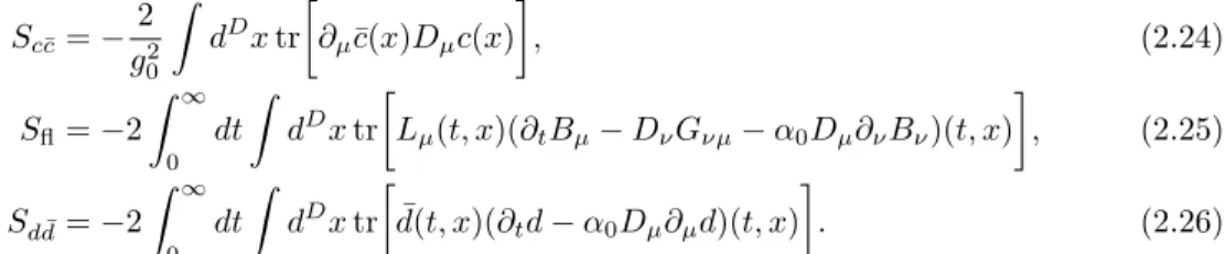
Beside these two types of lines, there are two types of “flow vertices” in Fig. 2.3 and Fig. 2.4 indicated by white blobs. These flow vertices arise fromXµ^(2)aandXµ^(3)a in Eqs. (2.15) and (2.16), respectively. There also exist “ordinary” vertices that arise from the action of the original gauge theoryS =SYM+Sgf+Sc¯c. In the next section, we construct the action of gauge theory in the (D+ 1)-dimensional spacetime, introducing a new fieldLµ(t, x), that reproduces the flow line, the flow propagator, the flow vertices, and the ordinary Yang–Mills vertices.

2.2 (D + 1)-dimensional gauge theory that reproduces the flow Feynman rules

For later discussion, we construct the (D+1)-dimensional action that reproduces the above Feynman rules for the flow Feynman diagrams. We then argue the property of needed counterterms for this (D+ 1)-dimensional theory that removes UV divergences.

First, we consider the flowed gauge field Bµ(t, x) as if it is an independent degrees of freedom in a (D+ 1) dimensional gauge theory. The action consists of two parts,S_D andS_D+1:

S=S_YM+S_gf+S_c¯_c

| {z }

S_D

+S| {z }_fl+S_dd¯ S_D+1

, (2.21)

SYM=− 1 2g²₀

∫

d^Dxtr [Fµν(x)Fµν(x)], (2.22)

Sgf =−λ0

g²₀

∫

d^Dxtr [

∂µAµ(x)∂νAν(x) ]

, (2.23)

(15)

CHAPTER 2. PROOF OF THE RENORMALIZABILITY OF THE GRADIENT FLOW 13

Figure 2.3: One of flow vertices arises from Xµ^(2)a in Eq. (2.15).

Figure 2.4: One of flow vertices arises from Xµ^(3)a in Eq. (2.16).

S_c¯_c=−2 g₀²

∫

d^Dxtr [

∂_µc(x)D¯ _µc(x) ]

, (2.24)

Sfl=−2

∫ _∞

0

dt

∫

d^Dxtr [

Lµ(t, x)(∂tBµ−DνGνµ−α0Dµ∂νBν)(t, x) ]

, (2.25)

S_dd¯=−2

∫ _∞

0

dt

∫

d^Dxtr [

d(t, x)(∂¯ td−α0Dµ∂µd)(t, x) ]

. (2.26)

The first part SD is just the D dimensional Yang–Mills theory with the gauge fixing term in Eqs. (2.19) and (2.20). Sfl contains the (D+ 1)-dimensional freedomLµ(t, x) andBµ(t, x), where Lµ(t, x) is a Lagrange multiplier. After integrating overLµ(t, x), the functional integral overBµ(t, x) is restricted to the solution of the flow equation 2.4; the boundary conditionBµ(t= 0, x) =Aµ(x) has to be assumed later. S_dd¯is on the other hand composed from ¯d(t, x) andd(t, x), whered(t, x) is a (D+ 1)-dimensional ghost and ¯d(t, x) is a Lagrange multiplier that imposes the flow equation,

∂td=α0Dµ∂µd(t, x), d(t= 0, x) =c(x). (2.27) We can easily show that this (D+ 1)-dimensional actionS reproduces the Feynman rules for flow Feynman diagrams in the previous section. The rules of ordinary vertices (denoted by black blobs) are read oﬀ fromS_D. The flow vertices come from S_fl, especially fromLB²,LB³ terms:

• LBB∫_∞ vertex

0 dt∫

d^Dx L^a_µXµ^(2)a

• LBBB∫_∞ vertex

0 dt∫

d^Dx L^a_µXµ^(3)a

These flow vertices are denoted by white blobs as noted already. The flow line (the heat kernel)

(16)

CHAPTER 2. PROOF OF THE RENORMALIZABILITY OF THE GRADIENT FLOW 14 now corresponds to theLBpropagator, the inverse of the coeﬃcient ofLB term inSfl.

(δµρ∂t−δµρ∂_σ^x∂_σ^x−(α0−1)∂_µ^x∂_ρ^x)⟨B_ρ^a(t, x)L^b_ν(s, y)⟩^tree=δ^abδµνδ(t−s)δ(x−y)

⟨B_µ^a(t, x)L^b_ν(s, y)⟩^tree=δ^abθ(t−s)K_t₋_s(x−y)_µν (2.28) The LB propagator is denoted by an arrow that goes from L to B. One can see that any flow Feynman diagram drawn with these vertices and lines has a same value as the flow Feynman diagram drawn with the rules in the previous section. FromS_dd¯, we also have the following additional vertex and propagators for the flowed ghost fields,

• the flow line for the ghost field= ¯ddpropagator

⟨d¯^a(t, x)d^b(s, y)⟩^tree=δ^abδ(t−s)∫

pe⁻^α⁰^(t⁻^s)p²

• the flow propagator for the ghost field

⟨d¯^a(t, x)d^b(s, y)⟩^tree=δ^ab∫

pe⁻^α⁰^(t+s)p²e^ip(x⁻^{y) 1}_p₂

• ddB∫¯_∞ flow-vertex

0 dt∫

d^Dx α0f^abcd¯^aB_µ^b∂µd^c

These are necessary only to keep the BRS symmetry in the (D+ 1)-dimensional theory.

It is possible to show that counterterms that are needed for the cancellation of UV divergences arise in S_D only and S_D+1 does not need any renormalization. As the example, let us consider the two-point function of B^a_µ in the one-loop level. The flow Feynman diagrams that are relevant for ⟨B_µ^a(t, x)B_ν^b(s, y)⟩ are depicted in Fig. 2.5. After calculating these diagrams according

(a) (b) (c)

(d) (e) (f) (g)

Figure 2.5

to the Feynman rules,⟨B_µ^a(t, x)B_ν^b(s, y)⟩to the one-loop level turns out to be in the dimensional

(17)

CHAPTER 2. PROOF OF THE RENORMALIZABILITY OF THE GRADIENT FLOW 15 regularizationD= 4−2ϵ(this is the expression for the gauge groupG=SU(N)),

⟨B^a_µ(t, x)B_ν^b(s, y)⟩^{1 loop} =g²δ^ab

∫

p

e^ip(x⁻^y) 1 (p²)²

× {

(δ_µνp²−p_µp_ν)(1 +b₀

ϵg²)e⁻^(t+s)p² +λ⁻¹(1−c0−b0

ϵ g²)p_µp_νe⁻^α⁰^(t+s)p² }

, (2.29)

b0= N 16π²

11

3 , (2.30)

c0= N 16π²

(13 6 − 1

2λ )

. (2.31)

In addition to this, we also have the counterterm that arises from the substitutions (the one-loop level renormalization),

g₀²=µ^2ϵg² (

1−b0

ϵg² )

, (2.32)

λ₀= (

1−c₀ ϵ g²

)

λ, (2.33)

in the tree-level propagator,

⟨B_µ^a(t, x)B^b_ν(s, y)⟩^tree=g²₀δ^ab

∫

p

e^ip(x⁻^y) 1 (p²)²

{

(δµνp²−pµpν)e⁻^(t+s)p²+λ⁻₀¹pµpνe⁻^α⁰^(t+s)p² }

. (2.34) We see that UV divergences in ⟨B^a_µ(t, x)B_ν^b(s, y)⟩^{1 loop} are precisely cancelled by the counterterm.

This shows that in the one-loop level the parameter renormalization make⟨B_µ^a(t, x)B_ν^b(s, y)⟩^{1 loop} finite without any wave function renormalization.

We want to show that the above UV finiteness of the correlation functions of the flowed gauge field without the wave function renormalization persists, not only in the one-loop level, in all orders of perturbation theory.

First, we note that possible UV divergences occur only at the “boundary” of the (D + 1)- dimensional spacetime, i.e., at the zero flow timet= 0. This follows from the observation that in any loop in a flow Feynman diagram, if at least one of the flow times of flow vertices is non-zero, then the loop integral absolutely convergent, because of the Gaussian damping factor in the heat kernel or the flow propagator. For this, an important fact is that there is no loop consisting only of the heat kernel,⟨B^a_µ(t, x)L^b_ν(s, y)⟩^tree=δ^abθ(t−s)K_t₋_s(x−y)_µν; because of the step functionθ(t−s), such a loop is measured-zero and can be neglected. All UV divergences in the (D+ 1)-dimensional field theory occurs at the boundary att= 0.

Another crucial observation is that the 1PI diagram that contains the flowed gauge fieldBshould always accompanyLat least at one of external vertices. This follows from the above Feynman rule (the vertices containingB always accompany one L) and again from the fact that there is no loop consisting only of the heat kernel ⟨BL⟩. The only way to make a loop without any external L vertex is a loop consisting only of⟨BL⟩lines, but this is impossible.

A similar statement holds for the (D+1)-dimensional ghostd; possible UV diverging 1PI vertices are at the zero flow time and it must accompany at least one Lagrange multiplier ¯dat least at one of external vertices.

(18)

CHAPTER 2. PROOF OF THE RENORMALIZABILITY OF THE GRADIENT FLOW 16 From these considerations and from the fact that the divergent part must be a local polynomial of fields of the mass dimension 4 and the ghost number 0, we see that the most general form of the divergent part which contains (D+ 1)-dimensional fields is (in thel-th loop level),

2g^2l

∫

d^Dxtr [

z₁L_µ(0, x)A_µR(x) +z₂d(0, x)c¯ _R(x) ]

, (2.35)

where we have noted the boundary conditions,B(t= 0, x) =A_Rµ(x) andd(t= 0, x) =c_R(x).

On the other hand, it turns out that the above (D+1)-dimensional gauge theoryS=S_D+S_D+1 is invariant under the BRS transformations of the form,

δ_BRSB_µ=D_µd, (2.36)

δBRSLµ = [Lµ, d], (2.37)

δBRSd=−d^ad^bT^aT^b, (2.38)

δBRSd¯=DµLµ− {d, d}. (2.39) We now show that the counterterm (2.35) cannot exist by the restriction implies by the BRS invariance. From the BRS invariance, we have following Ward–Takahashi (WT) relations:

λ₀⟨B_µ^a(t, x)∂_νA^b_ν(y)∂_ρA^c_ρ(z)⟩=−⟨(D_µd)^a(t, x)¯c^b(y)∂_ρA^c_ρ(z)⟩, (2.40) because the action and the functional integration measure are BRS invariant. Under the standard renormalization in the original Yang–Mills theory,

λ⟨B_µ^a(t, x)∂νA_νR^b (y)∂ρA^c_ρR(z)⟩=−⟨(Dµd)^a(t, x)¯c^b_R(y)∂ρA^c_ρR(z)⟩. (2.41) The counterterm (2.35) further contributes to both sides of the WT identity (2.40) through the tree-level diagrams in Fig. 2.6. From Fig. 2.6, we see that the counterterm (2.35) contributes to the left-side by 3z1g^2l while to the right-side by [(z1+z2) + (z1+z2) +z2]g^2l = (2z1+ 3z2)g^2l. Thus the WT identity for the BRS symmetry in the l-loop order implies z1 = z2 = 0. There is no need of the counterterm of the form (2.35). Only counterterms needed is the counterterms in the original ordinary YM theory. This shows in particular that there is no need of the wave function renormalization of the flowed gauge field. It can be seen this UV finiteness persists even for composite operators (i.e., the local products) of the flowed gauge field. The crucial point is again that there is no closed loop being consisting the heat kernels.

In Ref. [14], it is claimed that for t → 0, where t is the flow time, any composite operator (i.e., the local product) of the flowed field can be expressed by an asymptotic series of composite operators of the un-flowed field with increasing mass dimensions. Thissmall flow-time expansion works, for example, for the following gauge invariant dimension 4 operator,

E(t, x) = 1

4G^a_µν(t, x)G^a_µν(t, x). (2.42) as

E(t, x) =⟨E(t, x)⟩+c_E(t){1

4F_µν^a F_µν^a }R(x) +O(t). (2.43) The first term is the unit operator and the second term is a renormalized operator of the dimension 4 at the zero flow time. The last O(t) represents the contribution of operators of the dimension 6

(19)

CHAPTER 2. PROOF OF THE RENORMALIZABILITY OF THE GRADIENT FLOW 17

(a) (b)

(c) (d)

(e)

Figure 2.6: The tree diagrams that are relevant to the contributions of the counterterm (2.35) to the both sides of Eq. (2.40). The diagrams (a) and (b) show the contributions to the left-hand side, while diagrams (c)–(e) show the contributions to the right-hand side. If the diagram has a B_µ(t ̸= 0, x)A_ν(y) line, it can be decomposed into B_µ(t ̸= 0, x)L_ρ(0, z) line and A_ρ(z)A_ν(y) line by using the two-point vertex g^2lz1Lµ(t = 0, x)Aν(x) in the first term of Eq. (2.35). The diagram with this decomposed BA line has the contribution of g^2lz1 times the value of the original diagram. For example, the diagram (a) has two BA lines and gives the contribution 2g^2lz1λ0⟨B^a_µ(t, x)∂νA^b_ν(y)∂ρA^c_ρ(z)⟩^tree to the left-hand side of Eq. (2.40). Similarly, if the diagram has a d(t ̸= 0, z)¯c(y) line, it can be decomposed to d(t ̸= 0, x) ¯d(0, z) andc(z)¯c(y). The diagram with this decomposedd¯cline has the contribution of g^2lz2times the value of the original diagram.

(20)

CHAPTER 2. PROOF OF THE RENORMALIZABILITY OF THE GRADIENT FLOW 18 or higher. This small flow-time expansion provides a possible way to represent an operator in the original gauge theory in terms of composite operators of the flowed field that does not require the wave function renormalization. In Chap. 3 and Chap. 4, this technique will be fully utilized to find the expression of the supercurrent in terms of flowed fields.

(21)

Chapter 3

The 4D N = 1 super Yang–Mills theory

In Introduction, we mentioned the application of the gradient flow to the constructing of a regularization- independent expression for the energy–momentum tensor (EMT). In this section, we consider the construction of a regularization-independent supercurrent in terms of flowed fields in the simplest 4D supersymmetric gauge theory, theN = 1 SYM.

3.1 Action, super transformations, and BRS-invariance

We consider theN = 1 SYM in theDdimensional Euclidean spacetime. The action is given by S= 1

4g²₀

∫

d^Dx F_µν^a (x)F_µν^a (x) +1 2

∫

d^Dxψ¯^a(x) /D^abψ^b(x), (3.1) where

Dâbµ =δâb∂µ+Aâbµ(x), Aâbµ =fâcbA^c_µ, D/âb=Dâbµ γµ, (3.2) F_µνâ (x) =∂_µAâ_ν(x)−∂_νAâ_µ(x) +fâbcA^b_µ(x)A^c_ν(x). (3.3) As explained in Introduction, this is the expression in the Wess–Zumino (WZ) gauge and only the gauge field and the gaugino field exist. The SUSY transformation in the WZ gauge is non-linear and its explicit form is given by

δξAâ_µ(x) =g0ξγ¯ µψâ(x), (3.4) δ_ξψâ(x) =− 1

2g₀σ_µνξF_µν^a (x), (3.5)

δξψ¯^a(x) = 1 2g₀

ξσ¯ µνF_µν^a (x). (3.6)

WhenD= 4, noting the fact that both the gaugino field and the SUSY transformation parameterξ are the Majorana spinor ¯ψ=ψ^T(−C⁻¹), one can see that the action is invariant under the above

19

グラディエントフローによる正則化非依存な超カレントの構成