File Information Type Doc URL DOI Issue Date Citation Author(s) Title

Instructions for use

Title

Author(s)

Citation

Issue Date

DOI

Doc URL

Type

File Information

Late Pleistocene and Holocene Glaciations in the Nepal Himalayas and Their Implications for

Reconstruction of Paleoclimate

Thesis submitted for degree of Doctor of Philosophy by Katsuhiko ASAHI

Graduate School of Environmental Earth Science, Hokkaido University

2004

ii Abstract

Glacial landforms indicate the existence of the past glaciation, and the limits of glacier extent may suggest paleoclimatic conditions. Nevertheless, the lack of the numerical dating has poorly defined the history of glaciations throughout the Himalayas. In the last decade, new dating techniques were developed and started to be applied to the glacial deposits in the Western Himalayas. The Nepal Himalayas are governed by the strong summer monsoon environments; hence, summer monsoon precipitation plays an important role in glacier nourishment. When the geographical extent of the Himalayas is considered, however, the amount of winter precipitation, which is delivered by the westerlies, should be considered on the glaciation in western Nepal. The region of the Nepal Himalayas is particularly important because it makes the junction between the westward summer monsoon and eastward winter westerlies along the southern flank of the great Himalaya. A comparative study on the glaciation limit between eastern and western Nepal, therefore, will lead to understanding the relative importance of the monsoon and westerlies during the Last Glacial. This study aims to show the framework of the history of glaciations in the Nepal Himalayas with the aid of numerical dating, and can imply the paleoclimate during the Last Glacial. Two study areas of the Kanchenjunga and Khumbu Himals were selected from eastern Nepal, and three areas of the Chandi, Api, and Sisne Himals were selected from western Nepal.

This study first delineated detailed distribution maps of glacial landforms in

the entire part of each study area by aerial photograph interpretation and field

observation. The morphostratigraphy of the glacial landforms led to the

classification into five moraine complexes, which were recognized in each study

area. This configuration of glacial landforms could be recognized in each study

area. This classification was confirmed by relative dating methods, mainly based

on the weathering criteria of boulders on moraines. Absolute age, by optically

stimulated luminescence (OSL) and radiocarbon datings, and relative dating

constrained the history of glaciation. From younger to older order, the stages are

the LIA (Little Ice Age), Holocene, Late Glacial (correlated with the Younger

Dryas), LGM (Last Glacial Maximum), and the early substage of the Last Glacial

iii

which correlated with MIS 3. Even in the LGM, the terminal position of the glacier was somewhat enlarged compared with that of the present glaciers. This fact implies that the glaciation was restricted even during the LGM.

Glacial equilibrium line altitude (ELA) is the elevation where the

accumulation and ablation of a glacier are balanced. This is an appropriate indicator

for the glaciation and local climate. A comparison of ELA between the LGM and

the present can show that the relative climatic enhancement or weakness between the

monsoon and westerlies controlled the style and timing of glaciations in the Nepal

Himalayas. Distinguished higher altitudes of the maximum elevation of lateral

moraines (MELM) were used to estimate the ELAs during the LGM. During the

LGM period, the latitudinal profiles of ELA had the same inclination tendency

toward the south as present. It suggests that monsoon precipitation is likely to have

been a ruling resource over glacier accumulation. The inclination of ELAs had

been enhanced southward during the LGM in eastern Nepal, whereas the gradient

had been almost equal as today in western Nepal. This fact can imply that the

decreased precipitation in summer restricted the glaciation throughout Nepal, and

that the enhanced winter precipitation possibly maintained glaciers in western Nepal.

iv Acknowledgement

First of all, I would like to express my most gratitude to Dr. Teiji Watanabe, Graduate School of Environmental Earth Science, Hokkaido University, who has been my supervisor since the enrollment in doctoral course. He provided many suggestions, advices and encouragements throughout all stages of doctoral work.

I also wish to express my sincere appreciation to Professor Shuji Iwata, Department of Geography, Tokyo Metropolitan University. He has been constantly instructed me on geomorphology in the Himalayas since the initiative of my study.

I should extend my warmest gratitude to Professors Yugo Ono and Kazuomi Hirakawa, Graduate School of Environmental Earth Science, Hokkaido University, who made valuable suggestions throughout the course study. Thanks are also due to Dr. Takayuki Shiraiwa, Institute of Low Temperature Science, Hokkaido University, who made many valuable suggestions for this thesis. I am also indebted to Professor Takashi Nakata, Department of Geography, Hiroshima University, for his kind admission to study in western Nepal in 1995, even though it was a great risk for him. That opportunity commenced the decade-long study in Nepal to date.

Many parts of this study were carried out when I was dispatched to Tribhuvan University, Kathmandu, as a Research Fellow under the Asian Studies Program from the Ministry of Education, Science, Sports and Culture, Government of Japan, for three years since 1999. During that period I was affiliated with Central Department of Geography, Tribhuvan University, Kirtipur as a visiting researcher. Sincere thanks are due to Professor Vidya B.S. Kansakar and Dr.

Narendra R. Khanal for their constant help in Nepal.

This study owes much to the indispensable contribution of OSL dating by Dr.

Sumiko Tsukamoto, Department of Geography, Tokyo Metropolitan University, and

I wish to appreciate it very much. Dr. Lewis A. Owen, Department of Earth

Science, University of California, Riverside, gave a lot of useful advices and

inspirations for this study. In the initiative of the study, Dr. Hiroshi Yagi,

Yamagata University, kindly offered aerial photographs and field skill, Dr. Ben

Richards, Department of Geography, Royal Holloway, University of London,

instructed luminescence techniques. Dr. Rupert Bäumler, Technische Universität

v

München gave valuable suggestions on pedological knowledge. Many thanks go to Dr. Takanobu Sawagaki and the colleagues in the Laboratory of Geoecology, Graduate School of Environmental Earth Science, Hokkaido University. Their daily discussion and encouragement supported this work.

Thanks are also due to Drs. Daisuke Higaki, Kotaro Fukui, Messrs Hisao Shitashima, Naohiro Nakamura, Masaki Sano, for their generous assistance in the field. Members of the "Cryosphere Research in the Himalayas (CREH)" project, led by Professor Yutaka Ageta, Nagoya University, continuously supported and gave critical advice on various parts of my study in Nepal. My sincere appreciation should be extended to Nepalese colleagues who always assisted me. Especially, among them, Dr. Birbal Rana, Department of Meteorology and Hydrology, His Majesty's Government of Nepal, offered climatological data in Nepal. The officers in the Survey Department, His Majesty's Government of Nepal, kindly helped to access the aerial photographs and topographical maps. Local people generally allowed me to conduct field study with kind hospitality, even though an alien visitor possibly disturbed their territories.

Finally, I hearty thank my family, the patience for my ten-year long adventurous field life in total.

This study was partly supported by the following research grants: The Inoue

Field Science Research Fund through the Japanese Society on Snow and Ice; The

Sasagwa Scientific Research Grant from the Japan Science Society; Grant-in-Aid for

Scientific Research from the Japan Society for the Promotion of Science

(No.14000268); and The Research Grant in Global Environment 2003 from the

Asahi Breweries Academic Promotion Foundation, respectively.

vi

Late Pleistocene and Holocene Glaciations in the Nepal Himalayas and Their Implications for Reconstruction of Paleoclimate

Contents

Abstract... ii

Acknowledgement... iv

Chapter 1. Introduction... 1

1.1 Significance of the study on the past glaciation in the Nepal Himalayas.... 1

1.2 Previous studies and recent progress on the past glaciations in the Himalayas………... 2

1.2.1 Previous studies on the past glaciations in the Himalayas 1.2.2 Recent progress on the past glaciations in the Himalayas 1.3 Objectives of this study……… 6

Chapter 2. Physical settings of study area……….. 8

Chapter 3. Methods of the study………... 11

3.1 Determination of glacial landforms………. 12

3.1.1 Aerial photograph interpretation 3.1.2 Stage classification by morphostratigraphy 3.2 Relative dating for moraines……… 13

3.3 Numerical dating for glacial sediments………... 17

3.3.1 Radiocarbon dating 3.3.2 Optically stimulated luminescence dating 3.4 Determination of present and past ELA……….….. 22

Chapter 4. Chronology of glaciations since the Last Glacial……… 25

4.1 Eastern Nepal………..…. 25 4.1.1 Kanchenjunga Himal

4.1.2 Khumbu Himal

vii

4.2 Western Nepal……… 61

4.2.1 Chandi Himal 4.2.2 Api Himal 4.2.3 Sisne Himal 4.3 Possibility of lower glaciation in Nepal……….……. 81

4.4 Framework of glacial chronology of the Nepal Himalayas………. 83

4.4.1 Glacial chronology of the Nepal Himalayas 4.4.2 Comparison of the glacial chronology of the Nepal Himalayas and the Indian/Pakistan Himalayas and Karakoram 4.5 Summary………. 86

Chapter 5. Reconstruction of paleoclimate………. 89

5.1 Existing glaciers and present climate……….…...…... 89

5.2 The climate of the Nepal Himalayas during the LGM………. 92

5.2.1 Reconstruction of ELA during the LGM 5.2.2 Implication for reconstruction of paleoclimate 5.3 Summary……….……… 106

Chapter 6. Conclusions………..… 107

Preferences……… 109

viii Table of figures

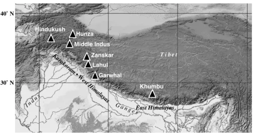
Figure 1.1 Locations of the Himalayan massifs with recent studies on timing

of glaciations, which are listed in Figure 1.2. 2 Figure 1.2 Glaciation histories proposed by previous studies within the

Himalayas based on numerical datings, correlated to the Oxygen

Isotopic Curve. 3

Figure 2.1 Locality of the study area in the Nepal Himalayas 8

Figure 3.1 Schema of the study methods 11

Figure 3.2 The scheme of rock weathering and oxidation with age to the right 14 Figure 3.3 Soil orders arranged into a development scheme on glacial

landforms, with age to the right 15

Figure 3.4 Significant correlation of Hurst soil colour indices between moist

and dry soils 16

Figure 3.5 Experimental process of preparation of methyl alcohol with liquid

scintillation for radiocarbon dating 18

Figure 3.6 Preparation procedure for coarse grained quartz and

potassium-rich feldspar 20

Figure 3.7 OSL dating method using single aliquot regenerative-dose (SAR)

protocol 20

Figure 3.8 Schematic dose response curve using SAR (Single Aliquot

Regenerative dose methods) protocol 21

Figure 4.1 Distribution map of glaciers and moraines in the Kanchenjunga

Himal 26

Figure 4.2 Detailed glacial geomorphological map in the vicinity of the

terminus of the Yalung Glacier, Kanchenjunga Himal 28

Figure 4.3 Cross section at Gyabla 30

Figure 4.4 Histograms of relative dating criteria for the Kanchenjunga Himal 32

Figure 4.5 Location of OSL dating sample collection 36

Figure 4.6 Section and log of OSL sample at Ramtang 39

Figure 4.7 Facis and log for OSL sample at Yamatari-tal 40

Figure 4.8 Locality, section, and log of OSL sample at Gyabla 41

Figure 4.9 Locality, section and log of OSL sampling at Nangartza 41

ix

Figure 4.10 Distribution map of glaciers and moraines in the Khumbu Himal 46 Figure 4.11 Detailed glacial geomorphological map in the vicinity of Periche,

Khumbu Himal 48

Figure 4.12 Detailed glacial geomorphological map in the vicinity of Chukung,

Khumbu Himal 49

Figure 4.13 Histograms of relative dating criteria for Imja Khola valley,

Khumbu Himal 52

Figure 4.14 Longitudinal profiles of the moraine surface and the present river

bed along the Khumbu Glacier 56

Figure 4.15 Locations of the glacial landforms where numerical age has been

assigned by the previous OSL and CRN dating studies 57 Figure 4.16 Distribution map of glaciers and moraines in the Chandi Himal 62 Figure 4.17 Histograms of relative dating criteria for Chandi Himal 64 Figure 4.18 Graphic sedimentary log of radiocarbon dating sample in Lare

Karlea, Chandi Himal 67

Figure 4.19 Schematic model of the sedimentary history in relation to glacial

fluctuations 68

Figure 4.20 Distribution map of glaciers and moraines in the Api Himal 71 Figure 4.21 Detailed glacial geomorphological map in the vicinity of Pil

Gandha 72

Figure 4.22 Histograms of relative dating criteria for the Api Himal 74 Figure 4.23 Distribution map of glaciers and moraines in the Sisne Himal 79 Figure 4.24 Distribution of glacial landforms in the upper Bhote Kosi

watershed in eastern Nepal 82

Figure 4.25 Summary of the glacial stages in the study area, Nepal Himalaya 84 Figure 4.26 Configuration model of the moraine complexes in the valley

glacations in the Nepal Himalayas 85

Figure 4.27 Correlation of the glaciation throughout the Himalayas and other

paleoclimatic proxy data 87

Figure 5.1 Variations of the present ELAs and the MELM in the LGM in the

Kanchenjunga Himal 90

Figure 5.2 Variations of the present ELAs and the MELM in the LGM in the

Khumbu Himal 90

x

Figure 5.3 Variations of the present ELAs and the MELM in the LGM in the

Chandi Himal and Api Himal 91

Figure 5.4 Variations of the present ELAs and the MELM in the LGM in the

the Sisne Himal 91

Figure 5.5 Variations of precipitations along the Kali Gandaki valley

crossing the Great Himalayas 92

Figure 5.6 Sites for the ELA reconstruction in the LGM by using MEG and

MELM methods in the Kanchenjunga Himal 94

Figure 5.7 Sites for the ELA reconstruction in the LGM by using MEG and

MELM methods in the Khumbu Himal 96

Figure 5.8 Photographs of the ELA reconstruction sites in the Khumbu Himal 98 Figure 5.9 Sites for the ELA reconstruction in the LGM by using MEG and

MELM methods in the Chandi Himal 99

Figure 5.10 Sites for the ELA reconstruction in the LGM by using MEG and

MELM methods in the Api Himal 100

Figure 5.11 Sites for the ELA reconstruction in the LGM by using MEG and

MELM methods in the Sisne Himal 101

Figure 5.12 Spatial variations of summer rainfall rate (A) and winter rainfall

rate (B) per annual precipitation in Nepal 105

xi Table of tables

Table 4.1 Results of relative dating methods adopted on glacial landforms in

the Kanchenjunga Himal 33

Table 4.2 Field description of the soils on the moraines and soil colour Index

(HCI) in the Kanchenjunga Himal 34

Table 4.3 A tentative glacial chronology of the Kanchenjunga Himal 38 Table 4.4 Summary of OSL/IRSL dating results: Location, material

description, radionuclide concentrations, moisture content, effective dose rate, equivalent dose and luminescence age from the

Kanchenjunga Himal, Nepal 42

Table 4.5 Measurement of the liquid scintillation radiocarbon dating of soils

and wood fragments in Kanchenjunga Himal 43

Table 4.6 Results of relative dating methods on glacial landforms in the Imja

Khola valley Khumbu Himal 53

Table 4.7 Field description of the soils on the HCI moraines and Soil Colour

Indicies in the Imja Khola valley, Khumbu Himal 54 Table 4.8 A tentative glacial chronology of the Khumbu Himal 56 Table 4.9 Numerical age on past glacations in the Khumbu Himal 58 Table 4.10 Radiocarbon ages of the buried soil, appeared in the lateral

moraines, in the Khumbu Himal reported in Röthlisberger (1986) 59 Table 4.11 Results of relative dating methods adopted on glacial land forms in

the Chandi Himal 65

Table 4.12 Field description of the soils on the moraines and Soil Colour Index

(HCI) in the Chandi Himal 66

Table 4.13 A tentative glacial chronology of the Chandi Himal 69 Table 4.14 Measurement of the liquid scintillation radiocarbon dating of soils

in the Chandi Himal 69

Table 4.15 Results of relative dating methods adopted on glacial landforms in

the Api Himal 75

Table 4.16 Field description of the soils on the moraines and Soil Colour

Indices (HCL) in Api Himal 76

Table 4.17 A tentative glacial chronology of the Api Himal 77

Table 4.18 Measurement of the liquid scintillation radiocarbon dating of soils

xii

in the Sisne Himal 80

Table 5.1 Reconstructed ELA during the LGM period in the Kanchenjunga

Himal 95

Table 5.2 Reconstructed ELAs during the LGM period in the Khumbu Himal 97 Table 5.3 Reconstructed ELAs during the LGM period in the Chandi Himal 97 Table 5.4 Reconstructed ELAs during the LGM period in the Api Himal 102

Table 5.5 Glacier inventory of the Sisne Himal 102

Table 5.6 Reconstructed ELA during the LGM period in the Sisne Himal 102

Chapter 1. Introduction

1.1 Significance of the study on the past glaciation in the Nepal Himalayas

The Nepal Himalayas can be characterized by the extensive coverage of high altitude glaciers that are more than approximately 5200 m in altitude. Glaciers in the Ice Age covered a wider area than those of the present, and many of the high altitude regions in the Nepal Himalayas have been glacierized before.

The Nepal Himalayas are governed by the strong summer monsoon environments; hence, summer monsoon precipitation plays an important role in glacier accumulation and fluctuation. The amount of winter precipitation that is delivered by the westerlies should be taken into consideration with regard to the glaciation in western Nepal. The region of western Nepal is particularly important because it forms the junction between the westward summer monsoon and the eastward winter westerlies along the southern flank of the great Himalayas. A study regarding glaciation in the past could reveal details of monsoon fluctuations in the Himalayas. Further, a comparative study on the glaciation limits of eastern and western Nepal will lead to an understanding of the relative importance of the monsoon and the westerlies during the Last Glacial.

Glacial landforms indicate the existence of past glaciation, and the limits of the glacier extent may suggest paleoclimatic conditions. Glacial morphostratigraphy and relative dating methods represent the timing of the glaciation, and the glacial advances may explain the history or the quantitative chronologies of glaciation throughout the Nepal Himalayas. Thus, a study based on the settings of glacial landforms and its dating provides a tentative framework for the history of the glaciations in the Nepal Himalayas.

Hence, a study based on the comparison between eastern and western Nepal is vital in order to provide a framework for the history of the glaciations in the Nepal Himalayas. The comparative study between eastern and western Nepal should reveal the past glaciation throughout the Nepal Himalayas.

An outline of the timing of glaciation in the Nepal Himalayas will shed light

on the timing and extent of the glaciation in the Great Himalayas throughout the Late

Quaternary. Furthermore, the chronology of glaciation by its timing and extent will enable a reconstruction of the paleoclimate of the Nepal Himalayas during the Last Glacial.

1.2. Previous studies and recent progress on the past glaciations in the Himalayas

The study of glaciation through the Last Glacial in the Himalayas has been attempted. Previous studies on the glaciation in the Himalayas have discussed the maximum extension of the glaciers and inferred age. Even though the chronologies of the glaciations in the Nepal Himalayas had been proposed, the age of each glacial advance in the region as well as throughout the Himalayas has not been adequately understood. This is partly because the dating of glacial landforms in the high Himalaya is problematic owing to the lack of organic materials for standard radiocarbon dating.

In the last decade, absolute dating methods for glacial sediments have been developed, and several studies on glacial history were conducted in the Himalayas.

The locations of the sites of recent studies on the timing of glaciations in the Himalayas are shown in Figure 1.1, and the proposed history with numerical dating is summarized in Figure 1.2.

Figure 1.1 Locations of the Himalayan massifs with recent studies on timing of glaciations, which are listed in Figure 1.2

..

Hindukush

Hunza Middle Indus

Zanskar Lahul

Garwhal

Khumbu

70˚ E 80˚ E 90˚ E 100˚ E

40˚ N

30˚ N

I nd us

G a ng e s

T i b e t Karakoram • West Himalayas

East Himalayas

Barum

Shandun

Pret

Drosh

Grabal 2 Shatial

Pasa II

Pasa I

Batura Ghulkin II

Ghulkin I

Borit Jheel

Sonapani

Kulti

Batal

Sonapani II

Sonapani I

Kulti Batal

Chandra

Bhujbas

Shuvling

Bhariathi

(a) (b) (c) (d) (e) (f) (g)

Lobche

Thuklha

Chhukung

Periche II Periche I Thyangboche II

(i)

3 3 2 2 1 5 4 5 4 4 3 2 5 4

Hindukush Middle- Indus Hunza Zanskar Lahul Garwhal Khumbu

Terminus altitude (km a.s.l.)

OSL OSL CRN OSL OSL, CRN OSL

0

10

100 2 4 6 8

20 40 60 80

Area/Dating method

1

OSL, CRN

1

2

3

4 5a 5b 5c

MIS

1 0 -1

Ocean

(SPECMAP)

δ

O

(‰)

Figure 1.2 Glaciation histories proposed by the previous studies within the Himalayas based on numerical datings, correlated to the Oxygen Isotopic Curve. The bars indicate terminus altitude of each glacial stage.

The width of the bar denotes the amplitude of the terminuses of the major glaciers. Corded bar indicates the undefined terminus in refences. Dark-coloured bar shows glacial stage defined by numerical dating.

Light-coloured bar shows glacial stage inferred with relative dating data. The locality of each Himalayan massifs should be referred to Figure 1.1. a) the Hindukush Mountains (data from Owen et al., 2002); b) The middle Indus valley (data from Richards et al., 2000a); c) the Hunza valley (data from Owen et al., 2000, Philips et al., 2000); d) the Zanskar range (data from Taylor and Mitchell, 2000); e) the Lahul Himalaya (data from Owen et al., 1996, 1997, 2001); f) the Garwhal Himalaya (data from Sharma and Owen, 1996); g) the Khumbu Himal (data from Röthlisberger, 1986, Richards, 2000b, Finkel et al, 2003);

i) Oxygen Isotopic Stage (data from Martinson et al., 1987).

1.2.1. Previous studies on the past glaciations in the Himalayas

The previous studies on the past glaciations in the Himalayas should be summarized in the following stages: Glacial advances in the Last Glacial Maximum (LGM); MIS 3 and 4 glaciations; and Large glacial extent in MIS 3/4 than MIS 2.

Glacial advances in the Last Glacial Maximum (LGM)

The major glacial advances during the Last Glacial Maximum (LGM) have not been confirmed in Hindukush, Zanskar and Garwhal Himalaya (Sharma and Owen, 1996; Taylor and Mitchell, 2000; Owen at al., 2002a). For example, Sharma and Owen (1996) proposed only one glacial advance, named the Bharirathi, in Garwhal Himalaya which they dated at 63 ka, using OSL. They identified a single long lateral moraine system. However, the lateral moraine system connected to the dated terminal moraine seems to be formed by at least two separate advances. This implies the existence of another glacial advance in the Garwhal Himalaya. Owen et al. (2001) revised the age of the Kulti Glacial stage using CRN at 10.6-11.4 ka.

They also revised the age of the Batal II Glacial stage and gave the age of 12-15.5 ka using cosmogenic dating. Both these records, especially the latter, could represent deglaciation from a LGM advance. The Batal II advance incorporates at least two moraine systems (Owen at al., 1997). Although Owen et al. (2001) did not mention these two moraines in their new chronology; the older moraine of the Batal stage could correspond to a glacial advance at the LGM (tentatively called Batal IIa).

Glacial advances occurred between 25 and 18 ka in the Middle Indus (Richards et al., 2000a) and Hunza Valley (Owen et al., 2002 b) of the Karakoram Mountains, and in Khumbu Himal (Richards et al., 2000b) and Kanchenjunga Himal (Tsukumoto et al., 2002) of the Nepal Himalayas. These data strongly support the idea of widespread glacier cover over much of the Karakoram and Himalayas in this time interval.

MIS 3 and 4 glaciations

Recent progress in OSL and CRN datings of glacigenic sediments and

landforms revealed that glacier advances occurred in MIS 3 and 4 in the Himalayas

and the Tibetan Plateau. MIS 4 glaciations are documented for the Middle Indus

(Grabal 2 stages; 70-65 ka: Richards et al., 2000a), Hunza (Borit Jheal Stage;

70-60ka: Owen et al., 2002b) and Garwhal Himalaya (Bharirathi Stage:>63ka:

Sharma and Owen, 1996). A latter part of the Batal Stage (dated 78 ka: Taylor and Mitchell, 2000) in Zanskar can also be assigned to MIS 4.

Glacial advance in the MIS 3 has been less ascertained with numerical dating in the Nepal Himalayas. However, in the Khumbu Himal, Iwata (1976) proposed Thyangboche Stage inferred to the early substage during the Last Glacial Period. Recently Finkel et al. (2003) confirmed with CRN dating that glacial advance was constrained in 35 ± 3 ka. Therefore, it is a subject to confirm the distribution of the moraines in this old stage by the interpretation of aerial photographs.

1.2.2. Recent progress on past glaciations in the Nepal Himalayas

The mapping of the geomorphic evidences revealed that the extent of glaciation in the Himalayan regions varied considerably throughout the Late Quaternary (Owen et al., 1998). Nevertheless, quantitative chronologies of the past glaciations in the Himalayas have been completely lacking. For example, in the Khumbu Himal, the relative glacial chronologies have been proposed by several authors (e.g., Iwata, 1976; Fushimi, 1977, 1978; Müller, 1980; Williams, 1983).

Most studies provide evidence of the glaciations and also their timing and extent.

However, the quantitative chronologies are rather inconclusive with regard to the past glaciations in the Himalayas (Owen et al., 1998; Richards et al., 2000).

According to Owen (1994), multivariate study of the sedimentology of deposits such as

C dates from organic materials is required before the genesis of a landform can be stated. The scarcity of organic materials in the sediments, which are generally deposited in high mountainous environments, precludes the utilization of standard radiocarbon dating techniques.

Thermoluminescence (TL) and optically stimulated luminescence (OSL) can be used to determine the time elapsed. Based on cosmogenic radionuclides (CRN) and OSL, the detailed glacial chronologies have not yet been completely established.

Here, controversy exists over the extent of former glaciations in many regions

throughout the Himalayas. This controversy arises mainly from the disagreement

regarding the interpretation of landforms that may be of either glacial or mass movement origin. These conflicting interpretations occur because the effects of intensive mass wasting can cause the misidentification of glacial landforms, mass movement landforms, and sediments with each other. Since the sediments that are involved in the process of mass movement and glaciation are very similar, they can easily be confused with each other in the absence of careful analysis (Gwen et al., 1998; Hewitt, 1999). Owen (1993) provides detailed descriptions of the nature of glacial and non-glacial diamictons to aid in the interpretation of glacial landforms in the Himalayas (Richard et al., 2002).

Recent advances in OSL and CRN surface exposure age dating have enabled the determination of the age of several glacial features. The OSL and CRN exposure dating in conjunction with new geomorphic and sedimentological analyses for selected regions of the Himalayas would enable the determination of the extent of glaciation during the LGM (Richard et al., 2002).

Further regional mapping and numerical dating are required to reconstruct and refine the pattern of glaciation throughout the high mountains of Central Asia.

Moreover, I strongly believe that detailed mapping of the glacial landforms in the entire region is essential not only to elucidate the classification of the glacial advanced stage by morphostratigraphy but also to determine the appropriate sites at which to collect OSL or CRN samples. Richard et al. (2001) highlighted the need for the use of multiple techniques and multi dating analyses to test method reliability.

Only after the completion of such systematic studies with respect to many more Himalayan regions will it be possible to produce a comprehensive map of the extent of glaciation in the Himalayas during the LGM and for other periods. As noted by Owen et al. (2002), it is necessary to adopt the relative dating methods, and careful and extensive field observations for improving the study on past glaciation in the Nepal Himalayas.

1.3 Objectives of this study

The major objective of this study is to provide a framework for the history of

the glaciation throughout the Nepal Himalayas. This is a comparative study on

glaciation in five study areas, i.e., two from eastern and three from western Nepal,

will lead to an understanding of the framework of glaciations in Nepal. First, this study aims to delineate a concrete mapping of glacial landforms and to clarify the classification of the moraine complex through aerial photograph interpretation and field observation. This classification is confirmed using relative dating methods.

Through absolute dating, this study attempts to ascertain the chronology of the glaciations in each study area of the Himalayan massif. Through these procedures, this study will show the framework of the history of glaciations in the Nepal Himalayas.

Another objective of this study is to imply the reconstruction of the paleoclimate during the Last Glacial. Equilibrium line altitude (ELA) is an appropriate indicator of glaciation and climate. The lowering ELAs compared between the east and west may imply relative changes in the monsoon and westerlies.

This study finally attempts to suggest the implication for the reconstruction of a past

climate during the LGM.

Chapter 2. Physical settings of study area

The Himalayas and the Tibetan Plateau constitute the largest glaciated mountain area outside of the Polar Regions ( 〜 126 200 km

: Haeberli et al., 1989;

Owen, et al., 2002). The Tibetan Plateau consists of 2 x 10

km

of land with an average surface elevation in excess of 4500 m a.s.l. (Fort, 1996; Richard, 1999).

The Himalayan Mountains (hereafter the Himalayas) comprises the southern flank of the Tibetan Plateau in the southern border. The Himalayas has been characterized by the existence of the glaciers in high altitudes. It rises approximately 5-7 km above the plains of the Indian subcontinent.

The Himalayas and the Tibetan Plateau influence on regional and global climate system (Benn and Owen, 1998; Owen et al., 2002). The Himalayan chain restricts the flow of moisture and air between these mountains regions. Orographic precipitation caused by the southernmost Himalaya depletes the moisture carried by summer monsoons, preventing moisture penetration to more northerly mountains (Pant and Kumar, 1992). Thus, the Nepal Himalayas is located under the strong summer monsoon environments, and monsoon precipitation plays an important role in glacier nourishment and fluctuation. Glacier advances in each of the regions are driven by local factors, most notably changes in monsoon and westerly circulation.

The Nepal Himalayas locates at the central part of the Himalayas stretches east westward between longitudes 80˚ and 88˚ east (Figure 2.1). This mountain range develops three major transverse river systems. They are; the Kosi, Gandaki,

Figure 2.1 Locality of the study area in the Nepal Himalayaa. The area with light-coloured

mesh shows over 4000 m a.s.l. and area with dark-coloured mesh denotes over 6000 m asl.

and Karnali, from east to west. Geographically, Nepalese territory can be divided into three regions according to these systems. Eastern, central, and western Nepal comprises the Kosi, Gandaki, and Karnali drainage basins, respectively.

This study selects the study areas two from eastern and three from western Nepal so that a comparative study between east and west leads to understand a framework for the history of glaciation in the Nepal Himalayas.

The eastern Nepal Himalayas develops the high mountain chain along the northernmost border. Among the 16 peaks exceed 8000 m high in the world, five peaks locates in this area. The modern glaciers extend linearly along the Great Himalaya range, and they cover the area of 1386 km

(Asahi, 1999). In the eastern Nepal, two areas are chosen; the Kanchenjunga and Khumbu Himals.

The Kanchenjunga Himal, which includes peaks higher than 8000 m in altitude, lies in the easternmost part of the Nepal Himalayas. Existing glaciers spread over the area almost more than 5000 m and the total glacierized area reaches 314 km

(Asahi, 1999). Well-developed moraines and tills in the entire part provide extensive evidences for the past glaciations. The Ghunsa valley and the Shimbuwa valley both originating from the peak of Kanchenjunga have well-developed landforms related to the past glaciation.

The Khumbu Himal is located in the eastern Nepal Himalayas that include Mt.

Everest and other peaks higher than 8000 m a.s.l. Numerous glaciers are located at greater approximately than 5000 m a.s.l. and the total glaciated area is 340 km

. Throughout the area, evidence of the past glaciations is apparent from well-developed moraines and glacial deposits. The distribution of the glacial landforms and the timing of past glaciations in this region have been argued since the 1970s.

The glacial history in western Nepal has not been defined to date. This is probably due to the most remote location in Nepal. The Himalayan mountains in western Nepal, with some exception, are constrained within almost 6000 m in altitude.

The modern glaciers, mainly consist of small mountain glaciers, are studded in the vast area. Less number of glaciers is mantled by thick debris on their surface.

It may reflect that glaciers in western Nepal nourished by different climatic situations,

such as strong insulation and aridity, compared with those in eastern Nepal. In this region, three areas are chosen; the Chandi, Api, and Sisne Himals.

The Chandi Himal locates near the northwestern corner of Nepal and about 15 km northeast from Simikot town. The Chandi Himal, which includes the highest peak of 6246 m a.s.l., contains small mountain glaciers along the central ridge of the mountains. The evidence of past glacialtion is partially preserved in moraine sequences in valleys.

The Api Himal, which includes the highest peak of 6246 m a.s.l., lies in the westernmost part of the Nepal Himalayas. The study area locates in the southern flank of the Himalayan range, and many of the existing glaciers developed on the south-facing slope. Throughout the study area, evidence of past glaciations is apparent from moraines, well-developed trough edge of U-shaped valley.

The Sisne Himal lies in the central southern part of the western Nepal that

includes the highest peak of 5582 m. Major parts of the mountain ridge are

constrained lower than 5000 m in altitude, and only six small glaciers stud on the

east-facing slope. The Sisne Himal locates 25 km east of Jumla town and next of

the Kanjiroba Himal to the west. Extensive evidences for the past glaciations are

provided by glacial landforms, such as cirque, moraine, and trough edge of U-shaped

valley.

Chapter 5

Reconstrction of paleoclimate

Chapter 4

Chronology of glaciations since the Last Glacial

Glacier inventory Glacier distribution map

Present ELA Past ELA

Reconstruction of paleoclimate during the LGM

Detailed map of glacial landform distribution

Aerial photograph interpretation

Field survey

Relative dating methods Classification of

moraine complex

Chronology of glaciations

Absolutel dating (OSL, ¹⁴C) Technique

Chapter 3 Methods of the study

This study at first delineated the geomorphic maps of glacial landforms using the latest aerial photographs of the entire part in each study area. The stratigraphical relationship and the configuration of these glacial landforms were classified into several moraine complexes. The stage classification of moraines was confirmed by relative dating methods, and numerical datings ascertained the ages of glacial advanced stages. Subsequently, the distinguished higher altitudes of the lateral moraines were selected from each area to reconstruct the ELA during the LGM. The comparison between ELAs of the present and the LGM imply relative changes in the paleoclimate of the Nepal Himalayas, especially between the monsoon and the westerlies (Figure 3.1).

Figure 3.1 Schema of the study methods

3.1 Determination of glacial landforms 3.1.1 Aerial photograph interpretation

At first, vertical aerial photographs of the entire part of each study area were interpreted using a stereoscope. The 1:50000 scale aerial photographs were taken by the Survey Department, Government of Nepal in 1992 for eastern Nepal and in 1996 for western Nepal. More than 800 photographs were investigated during this work. Glacial landforms, i.e., moraines and trough edges of U-shaped valley, were carefully delineated on topographic maps. Topographical maps were issued by the Survey Department from 1998 to 2002, throughout Nepal. The scale of this topographical map is 1:50000, and the contour interval is 40 m in the Himalayan region. A series of correct topographical sheets enabled an accurate description of the distribution of moraines in this work.

Reconnaissance field observation had been performed, except for the difficult case of reiterative field works, ahead of the aerial photograph interpretation. This field observation allowed for accurate and more detailed interpretation of the aerial photographs. The compilation of the geomorphic map was followed by the main field survey, and the map was supplemented accordingly so as to enable the completion of the distribution map of the moraines in each of the Himalayan massifs.

The interpretation and the determination of the glacial landforms were based on the criteria that the moraines and trough edges of U-shaped valley have clear continuity. For example, even if an abruptly appearing isolated mound in a valley appears to be a glacial moraine, there is a high probability of it having been developed by other geomorphic processes, such as landslides or rock avalanches in the Himalayas. One of the typical characteristics of landforms related to glaciation is continuity from an upper valley. Therefore, this study focused on the description of genuine “glacial” landforms in order to estimate the minimum lower limit of the glaciation during the Last Glacial.

3.1.2 Stage classification by morphostratigraphy

Delineated moraines of the entire region in each study area were divided into

several moraine complexes based on a geomorphic stratigraphy method resembling

that explained by Rose and Menzies (1996). In cases wherein a part of a moraine was topped by another moraine, the overlapped lower moraine must have been developed by the preceding glaciation. Thus, the configuration of the moraine, or the mutual position of the moraines, can evidence the temporal relationship between each moraine. Similarly, the geographic positions of moraines imply the relative, temporal differences of glacial advanced stages. During the field study, the morphostratigraphy of each moraine was precisely examined, and each of the widely spread moraines was assigned to a certain group of the moraine complex.

3.2 Relative dating for moraines

A relative chronology was established by techniques similar to those used by Burbank and Cheng (1991) for Mount Everest; Shiraiwa and Watanabe (1991) for the Langtang Valley; and Owen et al. (1996) for Lahul Himalaya. The adopted relative dating methods for boulders or clasts were mainly based on the weathering criteria. The sampling sites for relative dating were carefully selected from only at the top of the crest of a moraine ridge. This is to eliminate the possibility of considering boulders that have toppled or been displaced since the time of emplacement. A minimum of 50 boulders were examined at each site, and the values for each boulder were statistically analyzed in order to ascertain the site value of each method. The following relative dating methods were used: Schmidt hammer rebound value of the boulder surface; percentage of the clasts with oxidation stain; height of the mafic mineral projection; weathering pit depth; and thickness of the weathering rind on the clast surface. A lichenometric technique was also adopted on the surface of the same 50 boulders. The local geology of each study area predominantly consists of granite or gneiss. Data were collected only from granite rocks because of their distinct susceptibility to weathering. Simultaneously, pedological investigations, namely, soil profile development and soil colour development, were applied on the moraine crests.

A Schmidt hammer test applied to collect the rebound value (R-value) of

boulders is based on the scheme that rock weathered and weakened with age after the

release of a boulder from glacier ice (Figure 3.2). The R-value considered was the

mean value of three measurements for each of the 50 boulders. The site R-value for

each site was statistically calculated with the standard deviation.

The percentage of clasts with oxidation stain (Burke and Birkeland, 1979) was obtained for 50 boulders at each site. Rocks larger than 20 cm in diameter were cut off using a rock hammer. The rock with a discoloration of the gruss appeared in a section was recognized as oxidized rock, whereas a fresh surface in the section could be assigned as un-oxidized rock.

The height of the mafic mineral projection was measured on the boulder surface. Highly resistible mafic mineral in granite rock would remain prominently on the surface. The maximum value obtained from the 50 boulders was adopted.

However, it is necessary for the second maximum height to be larger than 80% of the maximum value in order to eliminate the transferred rocks after the emplacement of the moraine. The weathering pit depth was also based on the same logic of superficial weathering as that of the mafic mineral height. The maximum depth of the weathering pit observed on the 50 boulders was used.

The thickness of the weathering rind was measured at the same time as that of the calculation of the percentage of oxidized rock. Consequently, not much development of the rind could be found among the rocks throughout the Nepal Himalayas, and the rind value did not show contrast in the withering degree. The rind would possibly be affected by the characteristics of the resistance of granite rock in the High Himalaya.

Origin

weathering pit mafic mineral

projection

Rock oxidation:

slight; moderate; fully grus; weathering rind

Subsurface weathering Lichen

(Rhizocarpon Geographicum)

rounded surface

Figure 3.2 The scheme of rock weathering and oxidation with age to the right. A

theory on vegetation succession was also applied to the relative dating.

A theory on vegetation succession was also applied to the relative dating.

The lichenometric measurement was obtained from the 50 boulder surfaces of the abovementioned rocks. The maximum thallus diameters of the lichen "Rhizocarpon geographicum" were observed for the site value. Lichenometry can generally predict the assumptive age of moraines with the aid of the lichen growth curve.

However, to date, the lichen growth rate has not been advocated in the Nepal Himalayas. Therefore, this study applied only the maximum size of the inscribed diameter to differentiate the stages of the moraine complexes. Complementarily, the land coverage on the moraine crest was surveyed only in Khumbu Himal. The surface of the moraine, generally above the timberline, is composed of rock clasts and vegetation cover with lichens or moss. The surface coverage ratio of rock to vegetation was observed in this study.

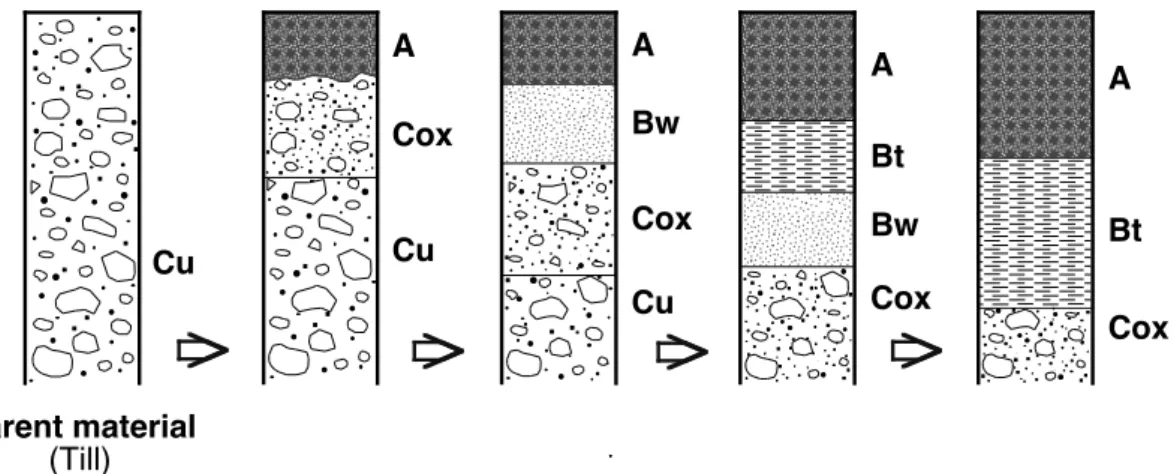
The soil profile development on the moraine was delimited so as to ascertain the maturity of the soil as supported by the nomenclature of Birkeland (1999). The comparison of soil profile development implies the rough estimation of the relative age after emplacement of the moraine (Figure 3.3). At the top of the moraine crest, an artificial pit was dug up to a C-horizon layer at each site. In addition, the soil colour indexes, namely, Hurst Soil Colour Index and Rubification Index (Birkeland, 1999), were calculated using soils from the same pit. The description and equation for calculating the index are described well by Birkeland (1999). With soil age, the Hurst Colour Index decreases whereas the Rubification Index increases. Both indexes are effective tools for identifying the stage difference within the Holocene

Cu

Parent material (Till)

A Cox

Cu

A Bw Cox Cu

A A

Bt

Bt Cox Bw

Cox

Figure 3.3 Soil orders arranged into a development scheme on glacial landforms, with

age to the right. Nomenclature is based on Birkeland (1999).

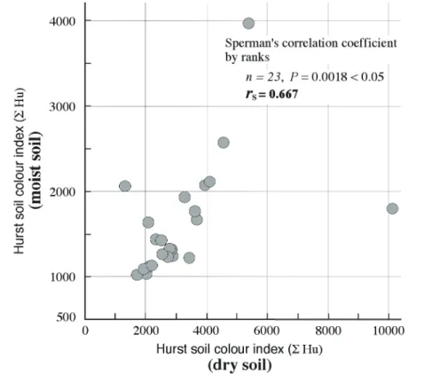
(Miller and Birkeland, 1974). The depth of the observation pit was unified in each study area. For the Hurst Colour Index, Hurst (1977) used dry colour for calculation, whereas Shiraiwa and Watanabe (1991) used moist colour. In this study, dry colour was used in Kanchenjunga Himal and Chandi Himal, while wet colour was used in Khumbu Himal and Api Himal. In actuality, there are no critical differences in the principal of this method. Hurst soil colour indexes at the same sites in Khumbu Himal, calculated by both dry and wet soil, were compared.

Sperman's correlation demonstrates a high coefficient (r

= 0.667), and a significant correlation of Hurst soil colour indexes between the moist and dry soils was verified (Figure 3.4).

The relative dating data obtained from each site were subjected to a statistical test in order to verify the significant differences among the moraine complexes.

This test is a non-parametric alternative to the two-sample Student’s t-test. The Mann-Whitney test was performed by combining the two data sets, sorting them in ascending order, and assigning each point to a rank. The Mann-Whitney test is compared to a table of critical values for U based on the sample size of each group. If U exceeds the critical value for U at some significance level (in this study: 0.05), it

Figure 3.4 Significant correlation of Hurst soil colour indeies between moist and

dry soils.

implies that there is evidence to reject the null hypothesis in favor of the alternative hypothesis.

3.3 Numerical dating for glacial sediments

According to the paucity of organic materials in relation to the past glaciations throughout the Himalayas, the timing of glaciation is poorly ascertained.

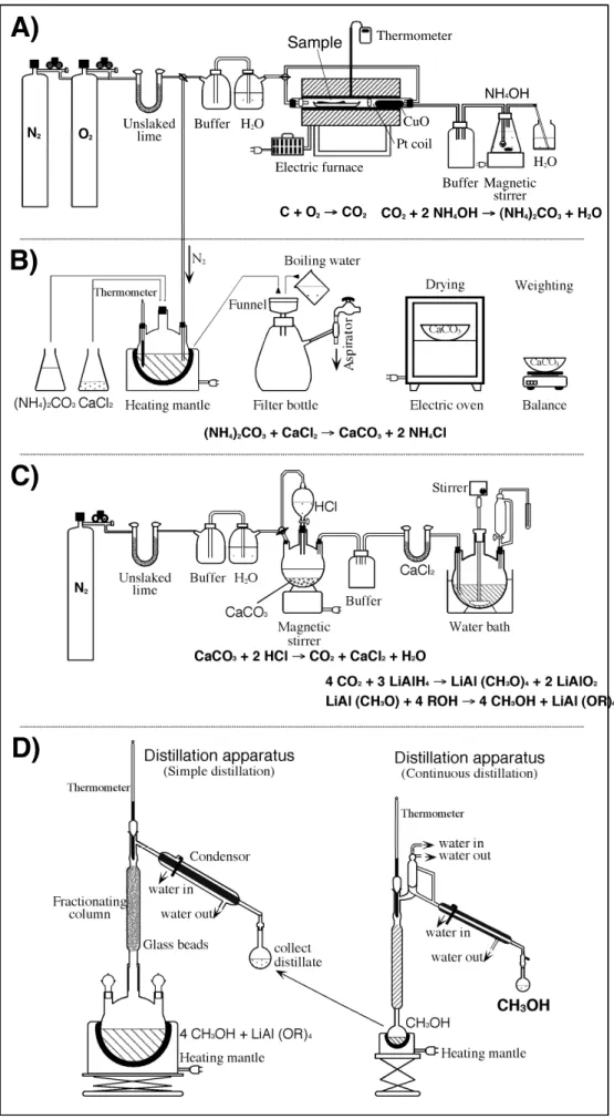
This study strived to obtain the ages of glaciation based on the detailed mapping of glacial landforms and reiterated field reconnaissance in each area. Radiocarbon and optically stimulated luminescence dating methods were adopted for this study.

3.3.1 Radiocarbon dating

Organic samples were collected to ascertain the timing of past glacations from several sites. Materials are: the wood fragment yielded within the terminal moraine; the buried soil mantled by Aeolian deposit developed on lateral moraines;

soil and peat dammed up by terminal moraine. Samples were electrically dried and contaminated materials, such as fibrous root, were carefully removed and sieved.

Pretreatment has been done by Acid, Acid-Alkaline, or Acid-Alkaline-Acid washes depending on the sample conditions. The liquid scintillation counting was used to radiocarbon dating in this work. Some samples were sent to Beta Analytic Inc., USA (Laboratory Code: "Beta") and others were analyzed by myself in the Department of Geography, Hiroshima University (Laboratory Code: "HU") using the methyl alcohol method. Sample preparation is conventional, and the process is summarized in Figure 3.5.

3.3.2 Optically stimulated luminescence dating

Absolute ages of the past glacial advances are poorly defined throughout the Himalayas. This is mainly because of the lack of dating method that is available on glacial landforms. Optically stimulated luminescence dating (OSL) methods, however, can be used to estimate the age of the last exposure to sunlight (Huntley et al., 1985), and they have the potential to date glacigenic sediments. Owen et al.

(1997) revised the glacial chronology in Lahul Himalaya (India), using OSL dating

4 CO²+ 3 LiAlH⁴→LiAl (CH³O)⁴+ 2 LiAlO² LiAl (CH³O) + 4 ROH→4 CH³OH + LiAl (OR)⁴ N2 O2

Buffer H2O Unslaked

lime

Buffer Magnetic stirrer Thermometer

Electric furnace

CuO Pt coil

H2O

Sample

NH⁴OH

C + O2→CO2 CO2+ 2 NH4OH→(NH4)2CO3+ H2O

A)

B)

C)

D)

Figure 3.5 Experimental process of preparation of methyl alcohol with liquid

scintillation for radiocarbon dating.

of glaciofluvial and glaciolacustrine sediments. They used only ice distal sediments because these sediments are more likely to have been bleached before deposition, rather than tills and ice proximal sediments. Sometimes, however, it is difficult to correlate ice distal sediments with particular glacial events. Richards et al. (2000) used glaciofluvial sediments interbedded between tills in the Khumbu Himal for OSL dating. The ages from different quartz size fractions and different samples collected adjacent to one another agreed well.

No published study exists on OSL dating of tills, but there are earlier TL works (i.e., Berger, 1984; Gemmel, 1988; Lamothe, 1988; Próoszynska-Bordas et al., 1988). In the Himalayas, many glaciers are covered by debris, and this material was later deposited as supraglacial tills after the ice was melted. Supraglacial meltout tills are likely to be bleached before deposition, because they have been transported on the surface of the glacier. In contrast, basal tills such as deformation till and subglacial meltout tills are not likely to have been exposed to sunlight and would not be bleached.

In this study, the ages of glacial sediment samples, including supraglacial meltout tills, deformation tills, and outwash deposits only from Kanchenjunga Himal are estimated by OSL dating using newly developed single aliquot regenerative-dose protocol (Murray and Wintle, 2000).

The samples were dried and sieved to obtain a sample of 75-125 mm fraction.

Dark minerals in the 75-125 mm fraction were separated with a magnetic separator, and then quartz rich fraction was isolated using a bromoform solution. The fraction was then treated with 46% hydrofluoric acid (HF) for 40 minutes and rinsed with water. The samples were mounted on 10 mm diameter aluminum discs using silicon oil (Silkospray). The amount of the samples on each disk was about 2.5 mg (Figures 3.6 and 3.7).

OSL measurements were performed on an automated Risø reader at the

School of Geography and Geology, McMaster University, with infrared (IR) laser

diodes (830 nm) and blue light emitting diodes (470±30 nm). Eighty percent diode

power was used for all samples. Emissions were filtered with three HOYA U-340

glass filters. Additionally, an aluminum plate with either 0.9 or 2 mm diameter

Figure 3.6 Preparation procedure for coarse grained quartz and potassium-rich feldspar

Figure 3.7 OSL dating method using single aliquot regenerative-dose (SAR) protocol (Murray and Wintle, 2000).

pinhole was used, when the OSL signals were too bright.

IRSL and blue light stimulated luminescence (BLSL) signals of the samples were measured to check the purity of quartz. Initial IRSL intensity of each sample was < 3% of that of BLSL after the IRSL; however, the IRSL count rate for the samples was not negligible (B10

counts/s). BLSL intensity after IRSL measurement was extremely high (B10

counts/s). The samples were etched with fluosilisic acid for 3 days, but IRSL intensity remained unchanged. The samples were next etched with 40% HF for 20 min, and were re-sieved. Then, both IRSL and BLSL intensity decreased significantly; IRSL intensity turned close to zero, and BLSL intensity was decreased from B10

to B10

counts/s for 8 mm mask size sample. This indicates that not only IRSL but also BLSL was emitted from feldspar contamination and/or microinclusions in the original quartz fraction. Then, the D

values of BLSL for the extra etched fraction (fraction A), and BLSL for the fraction

before the extra etching (fraction B) were compared.

The following single aliquot regenerative dose (SAR) protocol (Murray and Wintle, 2000) was applied to determine the equivalent dose (D

) of the samples (Figure 3.8). Aliquots for fraction B were stimulated by the blue light, and BLSL DE was obtained for fraction B. Those for fraction A were illuminated by IR laser to monitor the feldspar contamination, and then illuminated by the blue LED at steps 2, 5, 8 and 11 in the following protocol, as suggested by Banerjee et al. (2001).

1. Preheat 220˚C, 240˚C, 260˚C, 280˚C or 300˚C for 10 sec. (the same temperature is used throughout).

2. Natural OSL (L

) at 125˚C for 100 sec..

3. Give test dose (D

).

4. Cut heat to 160˚C.

5. Test dose OSL (T

) at 125˚C for 100 sec..

6. Regeneration dose D

; D

; D

; D

(= 0 Gy), and D

(D

= D

).

7. Preheat 220˚C, 240˚C, 260˚C, 280˚C or 300˚C for 10 sec..

8. Regeneration OSL (L

; L

; L

; L

; L

) at 125˚C for 100 sec..

9. Give test dose (D

).

10. Cut heat to 160˚C.

11. Test dose OSL (T

; T

; T

; T

; T

).

12. Repeat steps 6-10 four times.

Figure 3.8 Schematic dose response curve using SAR (Single Aliquot Regenerative

dose method) protocol.

D

values were obtained by plotting the sensitivity corrected OSL (R

; R

; R

; R

; R

; R

. L

=T

) versus regeneration dose (D

) and by taking the intersection of the corrected natural signal (R

=L

/T

) and the regenerated growth curve.

Preheat test was undertaken using fraction B for one of the pairs at each sample locality. Four aliquots were used for each preheat temperature, and 20 total aliquots at five different preheat temperatures were subjected to the above protocol.

The remaining sample of the pair for fraction B was studied with 10 aliquots at only 240˚C preheat. Twelve aliquots of fraction A were analyzed for 991109C, 991028B, and 991119B, while only six aliquots of fraction A were available for 991117B because of the limited sample amount. All aliquots for fraction A were preheated at 240˚C for 10 sec.

The beta and gamma dose rates were estimated from uranium, thorium and potassium concentrations measured by neutron activation analysis, using the conversion factors of Adamiec and Aitken (1998). Internal dose rate for feldspar originated from

K was estimated, assuming the K content in feldspars as 7±3%, because the maximum K content in feldspar is 13.3% in K-feldspar (KAlSi

O

), and then two sigma covers the range of K from 1% to 13%.

Water contents were estimated by averaging measured moisture contents from subsamples, and 75% errors of water contents were taken into account for age calculation except Location 4 in Figure 4.5, where the measured water content was 4.1% and ±4% error was used. The cosmic dose was calculated from the geomagnetic latitude and altitude of the sample location, using the method of Prescott and Hutton (1988).

OSL dates were calculated by dividing D

values by annual dose rate.

3.4 Determination of the present and past ELA

Glacial ELA is the elevation where the accumulation and ablation of the

glacier are balanced. This is generally regarded as the snowline altitude on the

glacier, and therefore, it is an appropriate indicator of glaciation and local climate. In

places where modern glaciers exist, the lowering altitude of ELA can be used as a

high resolution proxy of air temperature and precipitation changes. This study

addresses the ELA of the present glaciers in eastern and western Nepal, in

comparison with that of the Last Glacial ones. The aim of this study is to speculate on the climatic conditions during the LGM.

Present glacial equilibrium line altitude

The present ELA of each glacier was identified from the surface topography of glacier using the latest aerial photograph interpretation. This is the conventional method of estimating the present ELA, except in cases wherein mass balance was observed on a glacier. At first, the vertical aerial photographs of the entire of each study area were interpreted using a stereoscope. Aerial photographs were investigated at the same time along with the compilation work of the glacial geomorphological map in each area. The conditions of the existing glacier, i.e., its shape, terminus position, range of the debris-covered area, and the medium moraine on the glacier, were delineated on a topographical map. The maximum elevation of the debris-covered area can be an indicator of the present ELA. Along with the maximum altitude of the debris-mantle, the snowline on the glacier, i.e., the slope change from convex (ablation area) to concave (accumulation area), were also applied to estimate the present ELA. However, the shapes of the glaciers appearing in the Himalayas are generally complicated because of the steep topography. Thus, only reliable data were selected in this study, and among the existing 510 glaciers throughout the study areas, 189 of them (37%) were eligible for use in the estimation of the present ELA.

Past glacial equilibrium line altitude

The past ELA dealt with in this study is that of during the LGM. Previous

studies have adopted several methods to estimate the past ELA. Williams (1983)

used the accumulation area ratio (AAR) method in the Shorong Himal and Khumbu

Himal, and he estimated that the ELA was depressed by approximately 950 m in this

region. Duncan et al. (1998) calculated (ca. 500-650 m) the depression during the

Late Pleistocene from Central Nepal using the toe-to-headwall ratio (THAR) method

with the aid of a digital elevation map. More recent work by Burbank et al. (2003)

proposed that 500-1000 m lowering had occurred in the Annapurna Himal during the

LGM using the AAR method. Yamada and Iwata (1995) reported from western

Nepal that an approximately 1000 m depression was recognized using AAR. Hence, the THAR or AAR methods were commonly used to reconstruct the past ELA in the Nepal Himalayas; however, these methods serve as an appropriate technique for a simple cirque glacier or plateau glacier (Dahl and Nesje, 1992). Reconstructed ELA would be commonly overestimated in the Himalayas due to the steep topography and the influence of blown snow.

The methods proposed by Dahl and Nesje (1992) and Nesje and Dahl (2000)

have been applied in this study. These methods are the maximum elevation of

lateral moraine (MELM) and the medium elevation of glacier (MEG). This study

compiled a detailed distribution map of glacial landforms in each study area. The

stratigraphical relationship and the configuration of these moraines, however,

distinguish only those formed during the LGM, with the assistance of absolute and

relative datings. In this study, the distinguished higher altitudes of the MELM were

selected in order to estimate the ELAs during the LGM. The MEG was also applied

only to the small cirque glaciers developed during the LGM period, so as to confirm

that the reconstructed ELAs by both MELM and MEG have a good correlation. On

the basis of the compilation of the glacial geomorphological map that covers the

whole study area, this method can demonstrate the minimum amount of ELA

depression, and it implies paleoclimate practically, unlike in previous studies.