Inside the Muchnik Degrees II: The Degree Structures induced by the Arithmetical Hierarchy of Countably Continuous Functions

Inside the Muchnik Degrees II: The Degree Structures induced by the Arithmetical Hierarchy of Countably

Continuous Functions

K. Higuchi

Department of Mathematics and Informatics, Chiba University, 1-33 Yayoi-cho, Inage, Chiba, Japan

T. Kihara

School of Information Science, Japan Advanced Institute of Science and Technology, Nomi 923-1292, Japan

Abstract

It is known that infinitely many Medvedev degrees exist inside the Muchnik degree of any nontrivial Π

subset of Cantor space. We shed light on the fine structures in- side these Muchnik degrees related to learnability and piecewise computability. As for nonempty Π

subsets of Cantor space, we show the existence of a finite- ∆

-piecewise degree containing infinitely many finite-( Π

)

-piecewise degrees, and a finite-( Π

)

- piecewise degree containing infinitely many finite- ∆

-piecewise degrees (where ( Π

)

denotes the di ff erence of two Π

sets), whereas the greatest degrees in these three

“finite- Γ -piecewise” degree structures coincide. Moreover, as for nonempty Π

subsets of Cantor space, we also show that every nonzero finite-( Π

)

-piecewise degree in- cludes infinitely many Medvedev (i.e., one-piecewise) degrees, every nonzero countable-

∆

-piecewise degree includes infinitely many finite-piecewise degrees, every nonzero finite-( Π

)

-countable- ∆

-piecewise degree includes infinitely many countable- ∆

-piecewise degrees, and every nonzero Muchnik (i.e., countable- Π

-piecewise) degree includes in- finitely many finite-( Π

)

-countable- ∆

-piecewise degrees. Indeed, we show that any nonzero Medvedev degree and nonzero countable- ∆

-piecewise degree of a nonempty Π

subset of Cantor space have the strong anticupping properties. Finally, we ob- tain an elementary di ff erence between the Medvedev (Muchnik) degree structure and the finite- Γ -piecewise degree structure of all subsets of Baire space by showing that none of the finite- Γ -piecewise structures are Brouwerian, where Γ is any of the Wadge classes mentioned above.

Keywords: Π

class, Medvedev degree, Borel measurable function, countable continuity

2010 MSC: 03D30, 03D78, 03E15, 26A21, 68Q32

∗Corresponding author

Email addresses:[email protected](K. Higuchi),[email protected] (T. Kihara)

1. Summary 1.1. Introduction

This paper is a continuation of Higuchi-Kihara [29]. Our objective in this paper is to investigate the degree structures induced by intermediate notions between the Medvedev reduction (uniformly computable function) and Muchnik reduction (nonuni- formly computable function). We will shed light on a hidden, but extremely deep, structure inside the Muchnik degree of each Π

subset of Cantor space.

In 1963, Albert Muchnik [46] introduced the notion of Muchnik reduction as a partial function on Baire space that is decomposable into countably many computable functions. Such a reduction is also called a countably computable function, σ -computable function, or nonuniformly computable function. The notion of Muchnik reduction has been a powerful tool for clarifying the noncomputability structure of the Π

subsets of Cantor space [57–59, 61]. Muchnik reductions have been classified in Part I [29] by introducing the notion of piecewise computability.

Remarkably, many descriptive set theorists have recently focused their attention on the concept of piecewise definability of functions on Polish spaces, in association with the Baire hierarchy of Borel measurable functions (see [43, 44, 55]). Roughly speaking, if Γ is a pointclass (in the Borel hierarchy) and Λ is a class of functions (in the Baire hierarchy), a function is said to be Γ -piecewise Λ if it is decomposable into countably many Λ -functions with Γ domains. If Γ is the class of all closed sets and Λ is the class of all continuous functions, it is simply called piecewise continuous (see for instance [32, 36, 45, 50]). The notion of piecewise continuity is known to be equivalent to the ∆

-measurability [32]. If Γ is the class of all sets and Λ is the class of all continuous functions, it is also called countably continuous [44] or σ -continuous [54]. Nikolai Luzin was the first to investigate the notion of countable-continuity, and today, many researchers have studied this concept, in particular, with an important dichotomy theorem (see [51, 64]).

Our concepts introduced in Part I [29], such as ∆

-piecewise computability, are indeed the lightface versions of piecewise definability. This notion is also known to be equivalent to the e ff ective ∆

-measurability [50]. See also [5, 19, 38] for more information on e ff ective Borel measurability.

To gain a deeper understanding of piecewise definability, we investigate the Medvedev- and Muchnik-like degree structures induced by piecewise computable notions. This also helps us to understand the notion of relative learnability since we have observed a close relationship between lightface piecewise definability and algorithmic learning in Part I [29].

In Part II, we restrict our attention to the local substructures consisting of the de- grees of all Π

subsets of Cantor space. This indicates that we consider the rela- tive piecewise computably (or learnably) solvability of computably-refutable problems.

When a scientist attempts to verify a statement P, his verification will be algorithmi-

cally refuted whenever it is incorrect. This falsifiability principle holds only when P is

represented as a Π

subset of a space. Therefore, the restriction to the Π

sets can be re-

garded as an analogy of Popperian learning [11] because of the falsifiability principle.

From this perspective, the universe of the Π

sets is expected to be a good playground of Learning Theory [31].

The restriction to the Π

subsets of Cantor space 2

is also motivated by several other arguments. First, many mathematical problems can be represented as Π

subsets of certain topological spaces (see Cenzer and Remmel [15]). The Π

sets in such spaces have become important notions in many branches of Computability Theory, such as Recursive Mathematics [23], Reverse Mathematics [60], Computable Analysis [65], E ff ective Randomness [21, 48], and E ff ective Descriptive Set Theory [42]. For these reasons, degree structures on Π

subsets of Cantor space 2

are widely studied from the viewpoint of Computability Theory and Reverse Mathematics.

In particular, many theorems have been proposed on the algebraic structure of the Medvedev degrees of Π

subsets of Cantor space, such as density [13], embeddability of distributive lattices [3], join-reducibility [2], meet-irreducibility [1], noncuppability [12], non-Brouwerian property [28], decidability [16], and undecidability [56] (see also [30, 57–59, 61] for other properties on the Medvedev and Muchnik degree structures).

The Π

sets have also been a key notion (under the name of closed choice) in the study of the structure of the Weihrauch degrees, which is an extension of the Medvedev degrees (see [6–8]).

Among other results, Cenzer and Hinman [13] showed that the Medvedev degrees of the Π

subsets of Cantor space are dense, and Simpson [57] questioned whether the Muchnik degrees of Π

subsets of Cantor space are also dense. However, this question remains unanswered. We have limited knowledge of the Muchnik degree structure of the Π

sets because the Muchnik reductions are very di ffi cult to control. What we know is that as shown by Simpson-Slaman [62] and Cole-Simpson [17], there are infinitely many Medvedev degrees in the Muchnik degree of any nontrivial Π

subsets of Cantor space. Now, it is necessary to clarify the internal structure of the Muchnik degrees.

In Part II, we apply the disjunction operations introduced in Part I [29] to understand the inner structures of the Muchnik degrees induced by various notions of piecewise computability.

1.2. Results

In Part I [29], the notions of piecewise computability and the induced degree struc- tures are introduced. Our objective in Part II is to study the interaction among the structures P/F of F -degrees of nonempty Π

subsets of Cantor space for notions F of piecewise computability listed as follows.

• dec

[ Π

] also denotes the set of all partial functions on N

that are decompos- able into finitely many partial computable functions with Π

domains.

• dec

[ Π

] denotes the set of all partial functions on N

that are decomposable into finitely many partial computable functions with ( Π

)

domains, where a ( Π

)

set is the di ff erence of two Π

sets.

• dec

[ ∆

] denotes the set of all partial functions on N

that are decomposable

into finitely many partial computable functions with ∆

domains.

• dec

[ ∆

] denotes the set of all partial functions on N

that are decomposable into countably many partial computable functions with ∆

domains.

• dec

[ Π

] denotes the set of all partial functions on N

that are decomposable into finitely many partial computable functions with ( Π

)

domains.

• dec

[ Π

]dec

[ ∆

] denotes the set of all partial functions on N

that are decom- posable into finitely many partial ∆

-piecewise computable functions with ( Π

)

domains, where a ( Π

)

set is the di ff erence of two Π

sets.

• dec

[ Π

] denotes the set of all partial functions on N

that are decomposable into countably many partial computable functions with Π

domains.

The relationship among these notions is summarized as follows.

— P/dec^<ω_d [Π⁰₂] —

P/dec^<ω_p [Π⁰₁] — P/dec^<ω_d [Π⁰₁] — P/dec^<ω_p [∆⁰₂] P/dec^<ω_d [Π⁰₂]dec^ω_p[∆⁰₂] — P/dec^ω_p[Π⁰₂]

— P/dec^ωp[∆⁰₂] —

In Part I [29], we observed that these degree structure are exactly those induced by the ( α, β|γ )-computability.

• [C

]

denotes the set of all partial computable functions on N

.

• [C

]

denotes the set of all partial functions on N

learnable with bounded

mind changes.

• [C

]

denotes the set of all partial functions on N

learnable with bounded

errors.

• [C

]

denotes the set of all partial learnable functions on N

.

• [C

]

denotes the set of all partial k-wise computable functions on N

for some k ∈ N .

• [C

]

denotes the set of all partial functions on N

learnable by a team.

• [C

]

denotes the set of all partial nonuniformly computable functions on N

(i.e., all functions f satisfying f (x) ≤

x for any x ∈ dom( f )).

As in Part I [29], each degree structure P/ [C

]

is abbreviated as P

. Then, we have the following relationship among these notions.

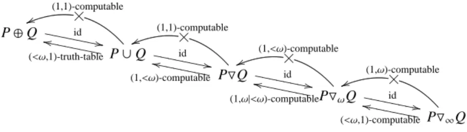
— P^<ω₁ —

P¹1 — P¹<ω — P¹_ω|<ω P^<ωω — P^ω1

— P¹_ω —

We will see that all of the above inclusions are proper. Beyond the properness of

these inclusions, there are four LEVELs signifying the di ff erences between two classes

F and G of partial functions on N

(lying between [C

]

and [C

]

) listed as follows.

1. There is a function Γ ∈ F \ G.

2. There are sets X , Y ⊆ N

such that F has a function Γ

: X → Y, but G has no function Γ

: X → Y.

3. There are Π

sets X , Y ⊆ 2

such that F has a function Γ

: X → Y, but Γ

has no function Γ

: X → Y.

4. For every special Π

set Y ⊆ 2

, there is a Π

set X ⊆ 2

such that F has a function Γ

: X → Y, but G has no function Γ

: X → Y.

The LEVEL 1 separation just represents F ⊈ G. Clearly, 4 → 3 → 2 → 1. Note that the LEVEL 2 separation holds for no Σ

sets X , Y ⊆ N

, since Π

is the first level in the arithmetical hierarchy which can define a nonempty set S ⊆ N

without computable element. Such a Π

set is called special, i.e., a subset of Baire space is special if it is nonempty and contains no computable points. As mentioned before, Simpson-Slaman [62] (see Cole-Simpson [17]) showed that the LEVEL 4 separation holds between [C

]

and [C

]

, that is, every nonzero Muchnik degree a ∈ P

contains infinitely many Medvedev degrees b ∈ P

.

In section 2, we use the consistent two-tape disjunction operations on Π

subsets of Cantor space introduced in Part I [29] to obtain LEVEL 3 separation results.

• ▽

is the disjunction operation on Π

sets induced by the two-tape Brouwer- Heyting-Kolmogorov-interpretation with mind-changes < n.

• ▽

is the disjunction operation on Π

sets induced by the two-tape Brouwer- Heyting-Kolmogorov-interpretation with finitely many mind-changes.

• ▽

is the disjunction operation on Π

sets induced by the two-tape Brouwer- Heyting-Kolmogorov-interpretation permitting unbounded mind-changes.

By using these operations, we obtain the LEVEL 3 separation results for [C

]

, [C

]

, [C

]

, and [C

]

. We show that there exist Π

sets P , Q ⊆ 2

such that all of the following conditions are satisfied.

1. (a) There is no computable function Γ

: P ▽

Q → P ▽

Q;

(b) There is a function Γ

: P ▽

Q → P ▽

Q learnable with bounded mind- changes.

2. (a) There is no function Γ

: P ▽

Q → P ▽

Q learnable with bounded mind- changes;

(b) There is a function Γ

: P ▽

Q → P ▽

Q learnable with bounded errors.

3. (a) There is no function Γ

: P ▽

Q → P ▽

Q learnable with bounded er- rors;

(b) There is a 2-wise computable function Γ

: P ▽

Q → P ▽

Q.

The above conditions also suggest how does degrees of di ffi culty of our disjunction operations behave.

In contrast to the above results, in section 3, we will see that the hierarchy be-

tween [C

]

and [C

]

collapses for homogeneous Π

subsets of Cantor space 2

.

In other words, the LEVEL 4 separations fail for [C

]

, [C

]

, and [C

]

. For

other classes, is the LEVEL 4 separation successful?

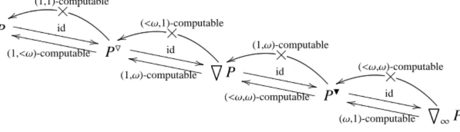
To archive the LEVEL 4 separations, we use dynamic disjunction operations de- veloped in Part I [29].

1. The concatenation P 7→ P

P of two Π

sets P ⊆ 2

indicates the mass problem

“solve P by a learning proof process with mind-change-bound 2”.

2. Every iterated concatenation along a well-founded tree indicates a learning proof process with an ordinal bounded mind changes.

3. The hyperconcatenation P 7→ P ▼ P of two Π

sets P ⊆ 2

is defined as the iterated concatenation of P along the corresponding ill-founded tree of P.

These operations turn out to be extremely useful to establish the LEVEL 4 separa- tion results. Some of these results will be proved by applying priority argument inside some learning proof model of P.

1. The LEVEL 4 separation succeeds for [C

]

and [C

]

, via the map P 7→ P

P.

2. The LEVEL 4 separation succeeds for [C

]

and [C

]

, via the map P 7→ ∪

m∈N

(P

P

. . . (m times) . . .

P

P) .

3. The LEVEL 4 separation succeeds for [C

]

and [C

]

, via the map P 7→ P ▼ P.

4. The LEVEL 4 separation succeeds for [C

]

and [C

]

, via the map P 7→

Deg(P), where d Deg(P) denotes the Turing upward closure of P. d

The method that we use to show the first and the third items also implies that any nonzero a ∈ P

and a ∈ P

have the strong anticupping property, i.e., for every nonzero a ∈ P , there is a nonzero b ∈ P below a such that a ≤ b ∨ c implies a ≤ c. Indeed, these strong anticupping results are established via concatenation

and hyperconcatenation ▼ .

1. P

| = ( ∀ a , c) (a ≤ (a

a) ∨ c → a ≤ c).

2. P

| = ( ∀ a , c) (a ≤ (a ▼ a) ∨ c → a ≤ c).

In section 5, we apply our results to sharpen Jockusch’s theorem [33] and Simp- son’s Embedding Lemma [58]. Jockusch showed the following nonuniform com- putability result for DNR

, the set of all k-valued diagonally noncomputable functions.

1. There is no (uniformly) computable function Γ

: DNR

→ DNR

. 2. There is a nonuniformly computable function Γ

: DNR

→ DNR

.

This result will be sharpened by using our learnability notions as follows.

1. There is no learnable function Γ

: DNR

→ DNR

.

2. There is no k-wise computable function Γ

: DNR

→ DNR

for k ∈ N . 3. There is a (uniformly) computable function Γ

: DNR

→ DNR

▼ DNR

. Hence,

there is a function Γ

: DNR

→ DNR

learnable by a team of two learners.

Finally, we employ concatenation and hyperconcatenation operations to show that

neither D

nor D

nor D

are Brouwerian. Hence, these degree structures are not

elementarily equivalent to the Medvedev (Muchnik) degree structure.

1.3. Notations and Conventions

For any sets X and Y, for convenience, we say that f is a function from X to Y (written f : X → Y) if the domain dom( f ) of f includes X, and the image of X under f is included in Y. We also use the notation f : ⊆ X → Y to denote that f is a partial function from X to Y, i.e., the image of dom( f ) ∩ X under f is included in Y.

For basic terminology in Computability Theory, see Soare [63]. For σ ∈ N

, we let |σ| denote the length of σ . For σ ∈ N

and f ∈ N

∪ N

, we say that σ is an initial segment of f (denoted by σ ⊂ f ) if σ (n) = f (n) for each n < |σ| . Moreover, f ↾ n denotes the unique initial segment of f of length n. let σ

denote an immediate predecessor node of σ , i.e. σ

= σ ↾ ( |σ| − 1). We also define [ σ ] = { f ∈ N

: f ⊃ σ} . A tree is a subset of N

closed under taking initial segments. For any tree T ⊆ N

, we also let [T ] be the set of all infinite paths of T , i.e., f belongs to [T ] if f ↾ n belongs to T for each n ∈ N . A node σ ∈ T is extendible if [T ] ∩ [ σ ] , ∅ . Let T

denote the set of all extendible nodes of T . We say that σ ∈ T is a leaf or a dead end if there is no τ ∈ T with τ ⊋ σ .

For any set X, the tree X

of finite words on X forms a monoid under concatenation

⌢

. Here the concatenation of σ and τ is defined by ( σ

τ )(n) = σ (n) for n < |σ| and ( σ

τ )( |σ| + n) = τ (n) for n < |τ| . We use symbols

and ⊓

for the operation on this monoid, where ⊓

i≤n

σ

denotes σ

σ

. . .

σ

. To avoid confusion, the symbols × and ∏

are only used for a product of sets. We often consider the following three left monoid actions of X

: The first one is the set X

of infinite words on X with an operation

: X

× X

→ X

; ( σ

f )(n) = σ (n) for n < |σ| and ( σ

f )( |σ| + n) = f (n) for n ∈ N . The second one is the set T (X) of subtrees T ⊆ X

with an operation

⌢

: X

× T (X) → T (X); σ

T = {σ

τ : τ ∈ T } . The third one is the power set P (X

)

of X

with an operation

: X

× P (X

) → P (X

); σ

P = {σ

f : f ∈ P } .

We say that a set P ⊆ N

is Π

if there is a computable relation R such that P = { f ∈ N

: ( ∀ n)R(n , f ) } holds. Equivalently, P = [T

] for some computable tree T

⊆ N

. Let {Φ

}

be an e ff ective enumeration of all Turing functionals (all partial computable functions

) on N

. Then the e-th Π

subset of 2

is defined by P

= { f ∈ 2

: Φ

( f ; 0) ↑} . Note that { P

}

is an e ff ective enumeration of all Π

subsets of Cantor space 2

. If (an index e of) a Π

set P

⊆ 2

is given, then T

= {σ ∈ 2

: Φ

( σ ; 0) ↑}

is called the corresponding tree for P

. Here Φ ( σ ; n) for σ ∈ N

and n ∈ N denotes the computation of Φ with an oracle σ , an input n, and step |σ| . Whenever a Π

set P is given, we assume that an index e of P is also given. If P ⊆ 2

is Π

, then the corresponding tree T

⊆ 2

of P is computable, and [T

] = P. Moreover, the set L

of all leaves of the computable tree T

is also computable. We also say that a sequence of { P

}

of Π

subsets of a space X is computable or uniform if the set { (i , f ) ∈ I × X : f ∈ P

} is again a Π

subset of the product space I × X. A set P ⊆ N

is special if P is nonempty and P has no computable member. For f , g ∈ N

, f ⊕ g is defined by ( f ⊕ g)(2n) = f (n) and ( f ⊕ g)(2n + 1) = g(n) for each n ∈ N . For P , Q ⊆ N

, put P ⊕ Q = ( ⟨ 0 ⟩

P) ∪ ( ⟨ 1 ⟩

Q) and P ⊗ Q = { f ⊕ g : f ∈ P & g ∈ Q } .

1In some contexts, a functionΦis called partial computable if it can be extended to someΦe. In this paper, we identify each partial computable function with such aΦe.

1.4. Notations from Part I 1.4.1. Functions

Every partial function Ψ : ⊆ N

→ N is called a learner. In Part I [29, Proposition 1], it is shown that we may assume that Ψ is total, and we fix an e ff ective enumeration {Ψ

}

of all learners. For any string σ ∈ N

, the set of mind-change locations of a learner Ψ on the informant σ is defined by

mcl

( σ ) = { n < |σ| : Ψ ( σ ↾ n + 1) , Ψ ( σ ↾ n) }.

We also define mcl

( f ) = ∪

n∈N

mcl

( f ↾ n) for any f ∈ N

. Then, #mcl

( f ) de- notes the number of times that the learner Ψ changes her / his mind on the informant f . Moreover, the set of indices predicted by a learner Ψ on the informant σ is defined by

indx

( σ ) = {Ψ ( σ ↾ n) : n ≤ |σ|}.

We also define indx

( f ) = ∪

n∈N

indx

( f ↾ n) for any f ∈ N

. We say that a partial function Γ : ⊆ N

→ N

is identified by a learner Ψ on g ∈ N

if lim

Ψ

(g ↾ n) converges, and Φ

(g) = Γ (g). We also say that a partial function Γ is identified by a learner Ψ if it is identified by Ψ on every g ∈ dom( Γ ). In Part I [29, Definition 2], we introduced the seven notions of ( α, β|γ )-computability for a partial function Γ : ⊆ N

→ N

listed as follows:

1. Γ is (1 , 1)-computable if it is computable.

2. Γ is (1 , < ω )-computable if it is identified by a learner Ψ with sup { #mcl

(g) : g ∈ dom( Γ ) } < ω .

3. Γ is (1 , ω| < ω )-computable if it is identified by a learner Ψ with sup { #indx

(g) : g ∈ dom( Γ ) } < ω .

4. Γ is (1 , ω )-computable if it is identified by a learner.

5. Γ is ( < ω, 1)-computable if there is b ∈ N such that for every g ∈ dom( Γ ), Γ (g) = Φ

(g) for some e < b.

6. Γ is ( < ω, ω )-computable if there is b ∈ N such that for every g ∈ dom( Γ ), Γ is identified by Ψ

for some e < b on g.

7. Γ is ( ω, 1)-computable if it is nonuniformly computable, i.e., Γ (g) ≤

g for every g ∈ dom( Γ ).

Let [C

]

(resp. [C

]

) denote the set of all ( α, β )-computable (resp. ( α, β|γ )-

computable) functions. If F be a monoid consisting of partial functions under com-

position, P ( N

) is preordered by the relation P ≤

Q indicating the existence of a

function Γ ∈ F from Q into P, that is, P ≤

Q if and only if there is a partial func-

tion Γ : ⊆ N

→ N

such that Γ ∈ F and Γ (g) ∈ P for every g ∈ Q. Let D/F and

P/F denote the quotient sets P ( N

) / ≡

and Π

(2

) / ≡

, respectively. Here, Π

(2

)

denotes the set of all nonempty Π

subsets of 2

. For P ∈ P ( N

), the equivalence

class { Q ⊆ N

: Q ≡

P } ∈ D/F is called the F -degree of P. If F = [C

]

for

some α, β, γ ∈ { 1 , < ω, ω} , we write ≤

, D

, and P

instead of ≤

, D/F and P/F .

The preorderings ≤

and ≤

are equivalent to the Medvedev reducibility [41] and the

Muchnik reducibility [46], respectively.

In Part I [29, Theorem 26 and Proposition 27], we showed the following equiva- lences:

P

= P/ dec

[ Π

] P

= P/ dec

[ ∆

] P

= P/ dec

[ ∆

] P

= P/ dec

[ Π

] P

= P/ dec

[ Π

]dec

[ ∆

] P

= P/ dec

[ Π

] Here, for a pointclass Λ , a function Γ : ⊆ N

→ N

is finite (countable, resp.) Λ -piecewise computable if there is a finite Λ -cover { X

}

(a uniform Γ -cover { X

}

, resp.) of dom( f ) such that Γ ↾ X

is computable for any i ∈ N , and the set of all finite (countable, resp.) Λ -piecewise computable functions is denoted by dec

[ Λ ] (dec

[ Λ ]). We denote by dec

[ Π

] the set of all finite Π

-layerwise computable func- tion (see Part I [29, Section 2.5]), which is equivalent to dec

[( Π

)

], where ( Π

)

is the complexity of the di ff erences of two Π

sets.

This observation allows us to think of each degree structure P

as a piecewise- degree structure in the following sense.

1. P

is the Medvedev degrees of Π

sets.

2. P

is the finite-( Π

)

-piecewise degrees of Π

sets.

3. P

is the finite- ∆

-piecewise degrees of Π

sets.

4. P

is the countable- ∆

-piecewise degrees of Π

sets.

5. P

is the finite-( Π

)

-piecewise degrees of Π

sets.

6. P

is the finite-( Π

)

-countable- ∆

-piecewise degrees of Π

sets.

7. P

is the Muchnik degrees (or equivalently, the countable- Π

-piecewise degrees) of Π

sets.

1.4.2. Sets

To define the disjunction operations in Part I [29, Definition 29], we introduced some auxiliary notions. Let I ⊆ N be a set. Fix σ ∈ (I × N )

, and i ∈ I. Then the i-th projection of σ is inductively defined as follows.

pr

( ⟨⟩ ) = ⟨⟩, pr

( σ ) = 

 pr

( σ

)

n , if σ = σ

⟨ (i , n) ⟩, pr

( σ

) , otherwise.

Moreover, the number of times of mind-changes of (the process reconstructed from a record) σ ∈ (I × N )

is given by

mc( σ ) = # { n < |σ| − 1 : ( σ (n))

, ( σ (n + 1))

}.

Here, for x = (x

, x

) ∈ I × N , the first (second, resp.) coordinate x

(x

, resp.) is denoted by (x)

((x)

, resp.). Furthermore, for f ∈ (I × N )

, we define pr

( f ) =

∪

n∈N

pr

( f ↾ n) for each i ∈ I, and mc( f ) = lim

mc( f ↾ n), where if the limit does not exist, we write mc( f ) = ∞ .

In Part I [29, Definition 33, 36 and 55], we introduced the disjunction operations.

Fix a collection { P

}

of subsets of Baire space N

. 1. ⟦ ∨

i∈I

P

⟧

= { f ∈ (I × N )

: (( ∃ i ∈ I) pr

( f ) ∈ P

) & mc( f ) = 0 } .

2. ⟦ ∨

i∈I

P

⟧

= { f ∈ (I × N )

: (( ∃ i ∈ I) pr

( f ) ∈ P

) & mc( f ) < n } . 3. ⟦ ∨

i∈I

P

⟧

= { f ∈ (I × N )

: ( ∃ i ∈ I) pr

( f ) ∈ P

} .

As in Part I, we use the notation write(i , σ ) for any i ∈ N and σ ∈ N

. write(i , σ ) = i

⊕ σ = ⟨ (i , σ (0)) , (i , σ (1)) , (i , σ (2)) , . . . , (i , σ ( |σ| − 1)) ⟩.

This string indicates the instruction to write the string σ on the i-th tape in the one / two- tape model. We also use the notation write(i , f ) = ∪

n∈N

write(i , f ↾ n) = i

⊕ f for any f ∈ N

.

In Part II, we are mostly interested in the degree structures of Π

subsets of 2

. As mentioned in Part I [29], the consistent disjunction operations are useful to study such local degree structures. The consistency set Con(T

)

for a collection { T

}

of trees is defined as follows.

Con(T

)

= { f ∈ (I × N )

: ( ∀ i ∈ I)( ∀ n ∈ N ) pr

( f ↾ n) ∈ T

}.

Then we use the following modified definitions. Fix a collection { P

}

of Π

subsets of Baire space N

and n ∈ ω ∪ {ω} .

1. [ `

n

]

i∈I

P

= ⟦ ∨

i∈I

P

⟧

∩ Con(T

)

. 2. [`

∞

]

i∈I

P

= ⟦ ∨

i∈I

P

⟧

∩ Con(T

)

.

Here T

is the corresponding tree for P

for every i ∈ I. If i ∈ { 0 , 1 } , then we simply write P

▽

P

, P

▽

P

, and P

▽

P

for these notions. In Part II, we use the following notion.

Definition 1. Pick any ∗ ∈ N∪{ω}∪{∞} . For each disjunctive notions ▽

and collection { P

}

of subsets of N

, fix the corresponding tree T

⊆ N

of P

for every i ∈ I and we may also associate a tree T

with (the closure of) P

▽

P

. Then the heart of P

▽

P

is defined by T

= {σ ∈ T

: ( ∀ i ∈ I) pr

( σ ) ∈ T

i

} .

Note that every σ ∈ T

is extendible in T

, since T

⊆ {σ ∈ T

: ( ∃ i ∈ I) pr

( σ ) ∈ T

i

} .

Let L

denote the set of all leaves of the corresponding tree for a nonempty Π

set P (where recall that such a tree is assumed to be uniquely determined when an index of P is given). Then the (non-commutative) concatenation of P and Q is defined as follows.

P

Q = P ∪ ∪

ρ∈LP

ρ

Q .

We also write T

T

for the corresponding tree of P

Q. Moreover, the commutative concatenation P ▽ Q is defined as (P

Q) ⊕ (Q

P). Let P and { Q

}

be computable col- lection of Π

subsets of 2

, and let ρ

denote the length-lexicographically n-th leaf of the corresponding computable tree of P. Then, we define the infinitary concatenation and recursive meet [3] as follows:

P

{ Q

}

= P ∪ ∪

n

ρ

Q

, ⊕

−→i∈N

Q

= CPA

{ Q

}

.

Here, CPA is a Medvedev complete set, which consists of all complete consistent ex- tensions of Peano Arithmetic. The Medvedev completeness of CPA ensures that for any nonempty Π

subset P ⊆ 2

, a computable function Φ : CPA → P exists.

In Part I, we studied the disjunction and concatenation operations along graphs.

For nonempty Π

subsets P and Q of 2

, the hyperconcatenation Q ▼ P of Q and P is defined by the iterated concatenation of P’s along the ill-founded tree T

, that is,

Q ▼ P =

 

 ∪

τ∈T_Q

 

 ⊓

i<|τ|

T

⟨τ (i) ⟩

 



T

 

 .

Note that, after writing this paper, Kihara [37] gave e ff ective topological interpre- tations of some of these constructions.

Remark. Recall from Section 1.3 that a corresponding tree of a Π

set is assumed to be uniquely determined when an index of the Π

set is given. Indeed, most of our above definitions obviously depend on our choice of indices (hence, corresponding trees) of given Π

sets, that is, most of operations introduced above are defined on subtrees of

N

rather than subsets of N

. Although there is no e ff ective well-defined map from

the Π

sets into the indices, it does not really matter what we chose, if we only focus on the degree-theoretic behavior. Formally, the reader should replace the words “for any (there exists a) Π

set” in this paper with “for any (there exitsts an) index of a Π

set”, or simply, the reader may suppose the definition of “a Π

set” to mean a structure P consisting of a pair of a Π

set P and its index e (or equivalently, its corresponding tree T

). We will frequently use index-dependent definitions in order to simplify our notations, but in each case, one can easily ensure that it cause no problems at all.

Contents

1 Summary 2

1.1 Introduction . . . . 2

1.2 Results . . . . 3

1.3 Notations and Conventions . . . . 7

1.4 Notations from Part I . . . . 8

1.4.1 Functions . . . . 8

1.4.2 Sets . . . . 9

2 Degrees of Di ffi culty of Disjunctions 12 2.1 The Disjunction ⊕ versus the Disjunction ∪ . . . . 13

2.2 The Disjunction ∪ versus the Disjunction ▽ . . . . 13

2.3 The Disjunction ▽ versus the Disjunction ▽

. . . . 15

2.4 The Disjunction ▽

versus the Disjunction ▽

. . . . 16

2.5 The Disjunction ⊕

versus the Disjunction `

. . . . 17

3 Contiguous Degrees and Dynamic Infinitary Disjunctions 20

3.1 When the Hierarchy Collapses . . . . 20

3.2 Concatenation, Dynamic Disjunctions, and Contiguous Degrees . . . 24

3.3 Infinitary Disjunctions along the Straight Line . . . . 28

3.4 Infinitary Disjunctions along ill-Founded Trees . . . . 31

3.5 Infinitary Disjunctions along Infinite Complete Graphs . . . . 34

4 Applications and Questions 37 4.1 Diagonally Noncomputable Functions . . . . 37

4.2 Simpson’s Embedding Lemma . . . . 39

4.3 Weihrauch Degrees . . . . 40

4.4 Some Intermediate Lattices are Not Brouwerian . . . . 42

4.5 Open Questions . . . . 45

Bibliography 46

2. Degrees of Di ffi culty of Disjunctions

The main objective in this section is to establish LEVEL 3 separation results among our classes of nonuniformly computable functions by using disjunction operations in- troduced in Part I [29, Sections 3 and 5]. We have already seen the following inequali- ties for Π

subsets P , Q ⊆ 2

in Part I [29, Section 5.1].

P ⊕ Q ≥

P ∪ Q ≥

P ▽ Q ≥

P ▽

Q ≥

P ▽

Q .

As observed in Part I [29, Section 4], these binary disjunctions are closely related to the reducibilities ≤

, ≤

, ≤

, ≤

, and ≤

, respectively. We employ rather exotic Π

sets constructed by Jockusch and Soare to separate the strength of these disjunctions. We say that a set A ⊆ N

is an antichain if it is an antichain with respect to the Turing reducibility ≤

. In other words, f is Turing incomparable with g, for any two distinct elements f , g ∈ A. A nonempty closed set A ⊆ N

is perfect if it has no isolated point.

Theorem 2 (Jockusch-Soare [35]). There exists a perfect Π

antichain in 2

.

A stronger condition is sometimes required. For a set P ⊆ N

and an element g ∈ N

, let P

denote the set of all element of P which are Turing reducible to g.

Then, a set A ⊆ N

is antichain if and only if A

= { g } for every g ∈ A. A set P ⊆ N

is independent if P

= D for every finite subset D ⊂ P.

Theorem 3 (see Binns-Simpson [3]). There exists a perfect independent Π

subset of 2

.

On the other hand, in Section 3.1, we will see that our hierarchy of disjunctions

collapses for homogeneous sets, which may be regarded as an opposite notion to an-

tichains and independent sets.

2.1. The Disjunction ⊕ versus the Disjunction ∪

We first separate the strength of the coproduct (the intuitionistic disjunction) ⊕ and the union (the classical one-tape disjunction) ∪ . This automatically establish the LEVEL 3 separation result between [C

]

and [C

]

. Recall that a set P ⊆ N

is special if it is nonempty and it contains no computable points.

Lemma 4. Let P

, P

be Π

subsets of 2

, and let Q be a special Π

subset of 2

. Assume that there exist f ∈ P

and g ∈ P

with Q

= Q

∪ Q

such that Q

and Q

are separated by open sets. Then Q ≰

(P

⊗ 2

) ∪ (2

⊗ P

).

Proof. Suppose that Q ≤

(P

⊗ 2

) ∪ (2

⊗ P

) via a computable functional Φ . Then f ⊕ g ∈ (P

⊗ 2

) ∪ (2

⊗ P

). By our choice of f and g, Φ ( f ⊕ g) must belong to Q

= Q

∪ Q

. By our assumption, Q

and Q

are separated by two disjoint open sets U , V ⊆ 2

. That is, Q

⊆ U, Q

⊆ V, and U ∩ V = ∅ . Therefore, either Φ ( f ⊕ g) ∈ Q ∩ U or Φ ( f ⊕ g) ∈ Q ∩ V holds. In any case, there exists an open neighborhood [ σ ] ∋ Φ ( f ⊕ g) such that [ σ ] ⊆ U or [ σ ] ⊆ V. Without loss of generality, we can assume [ σ ] ⊆ U. We pick initial segments τ

⊂ f and τ

⊂ g with Φ ( τ

⊕ τ

) ⊇ σ . Then ( τ

0

) ⊕ g ∈ (P

⊗ 2

) ∪ (2

⊗ P

), and it is Turing equivalent to g. However this is impossible because Φ ( τ

0

⊕ g) ∈ [ σ ], and [ σ ] ∩ Q

⊆ U ∩ Q

= ∅ . □ Corollary 5. 1. There are Π

sets P , Q ⊆ 2

such that P ∪ Q <

P ⊕ Q.

2. There are Π

sets P , Q ⊆ 2

such that P ≡

Q and P <

Q.

Proof. (1) Let R be a perfect independent Π

subset of 2

. Set P = 2

⊗ R and Q = R ⊗ 2

. Note that P ⊕ Q ≡

R. Pick f , g ∈ R such that f , g. Then R

= { f } , R

= { g } , and R

= R

⊔ R

= { f , g } . Since 2

is Hausdor ff , two points f and g are separated by open sets. Thus, P ⊕ Q ≡

R ≰

P ∪ Q by Lemma 4. (2)

P ⊕ Q ≡

P ∪ Q <

P ⊕ Q. □

Remark. One can adopt the unit interval [0 , 1] as our whole space instead of Cantor space 2

. Then, P

† P

: = (P

× [0 , 1]) ∪ ([0 , 1] × P

) is connected as a topological space. If P

⊆ [0 , 1] is homeomorphic to Cantor space, then the connected space P

† P

is sometimes called the Cantor tartan. The above proof shows that every perfect independent Π

set R ⊆ [0 , 1] is not (1 , 1)-reducible to the obtained tartan R † R, while these sets are ( < ω, 1)-tt-equivalent. Note that the tartan plays an important role on the constructive study of Brouwer’s fixed point theorem (see [10]).

2.2. The Disjunction ∪ versus the Disjunction ▽

We next separate the strength of the union ∪ and the concatenation (the LCM dis- junction with mind-change-bound 2) ▽ . Moreover, we also see the LEVEL 3 separation between [C

]

and [C

]

.

Lemma 6. Let P

, P

be Π

subsets of 2

, and let Q be a special Π

subset of 2

.

Assume that there exist f ∈ P

and g ∈ P

such that any h ∈ Q

and Q

are

separated by open sets. Then Q ≰

P

P

.

Proof. Suppose that Q ≤

P

P

via a computable functional Φ . By our choice of f ∈ P

⊆ P

P

, there must exist an open set U ⊆ 2

such that Φ ( f ) ∈ Q ∩ U and Q

∩ U = ∅ . Since U is open there exists a clopen neighborhood [ σ ] ∋ Φ ( f ) such that [ σ ] ∩ Q ⊆ U. We pick an initial segment τ ⊂ f with Φ ( τ ) ⊇ σ . Since f ∈ P

holds, we have that τ ∈ T

, and we pick ρ ∈ L

extending τ . Then ρ

g ∈ P

P

, and ρ

g is Turing equivalent to g. So, if Q ≤

P

P

via Φ , then Φ ( ρ

g) must belong to Q

. However this is impossible because Φ ( ρ

g) ∈ [ σ ], and [ σ ] ∩ Q

⊆ U ∩ Q

= ∅ . □ Corollary 7. There are Π

sets P , Q ⊆ 2

such that P

Q <

P ∪ Q <

P ⊕ Q.

Proof. Assume that R be a perfect Π

antichain of 2

. Set P = 2

⊗ R and Q = R ⊗ 2

. Pick f , g ∈ R such that f , g. Then R

= { f } and R

= { g } since R is antichain. Therefore, (P ∪ Q)

⊆ ( { X } ⊗ 2

) ∪ (2

⊗ { X } ) for each X ∈ { f , g } . For h = h

⊕ h

∈ (P ∪ Q)

, we have h

, g and h

, g. Thus, h < (2

⊗ { g } ) ∪ ( { g } ⊗ 2

), and note that (2

⊗ { g } ) ∪ ( { g } ⊗ 2

) is closed. Then, there is an open neighborhood U ⊆ 2

such that h ∈ U and U ∩ (P ∪ Q)

= ∅ , since P ∪ Q is regular, and (P ∪ Q)

⊆ (2

⊗ { g } ) ∪ ( { g } ⊗ 2

). Namely, any h ∈ (P ∪ Q)

and (P ∪ Q)

are separated by some open set. Consequently, by Lemma 6, we have P ∪ Q ≰

P

Q. □ One can establish another separation result for the concatenation. Recall from [12]

that a closed set P ⊆ N

is immune if T

contains no infinite c.e. subset. In [12] it is shown that the class of non-immune Π

subsets of Cantor space is downward closed in the Medvedev degrees P

. This property also holds in a coarser degree structure. In Part I [29, Section 2.4] we have seen that P

is an intermediate structure between P

and P

.

Lemma 8. Let P and Q be Π

subsets of 2

. If P is not immune, and Q ≤

P, then Q is not immune.

Proof. Let V be an infinite c.e. subset of T

. Assume that Q ≤

P holds via n truth- table functionals {Γ

}

. Note that every functional Γ

can be viewed as a computable monotone function from 2

into 2

. Let V

be the c.e. set V ∩ ∩

i<k

Γ

[2

\ T

] for each k ≤ n. By our assumption, V

is finite, since otherwise the tree generated from V has an infinite path f such that Φ

( f ) < P for every i < n. Let k be the least number such that V

is finite. Then, Γ

[V

] is an infinite c.e. set, and Γ

[V

] is included in T

except for finite elements. □

Corollary 9. There are Π

sets P , Q ⊆ 2

such that Q <

P ≡

Q.

Proof. Let P be an immune Π

subset of 2

. Put Q = P

P. As seen in Part I [29,

Section 4], we have Q ≤

P ≡

Q. Then, Q is not immune since T

includes an

infinite computable subset T

. Hence, P ≰

Q by Proposition 8. □

We have introduced two concatenation operations

and ▽ , while there are several

other concatenation-like operations (see Duparc [22]). For Π

sets P and Q, let P

Q

and P

Q denote [ {σ

♯

τ : σ ∈ T

& τ ∈ T

} ] and [ {σ

τ : σ ∈ T

& τ ∈ T

} ],

respectively. (Note that these definitions are also index-dependent, and recall that the

final remark in Section 1.4.2.) As seen in Part I [29, Proposition 53], we have P

Q ≡

P

Q. However, there is a (1 , 1)-di ff erence between P

Q and P

Q.