Study on An improvement of Numerical Association Rule Extraction for
Multi‑Objective Optimization Problem (Case studi: Bioelectric Potential Data)
著者 イマム タヒュディン
著者別表示 Imam Tahyudin journal or
publication title
博士論文本文Full 学位授与番号 13301甲第4824号
学位名 博士(工学)
学位授与年月日 2018‑09‑26
URL http://hdl.handle.net/2297/00053070
doi: 10.18494/SAM.2018.1887
DISSERTATION
STUDY ON AN IMPROVEMENT OF NUMERICAL ASSOCIATION RULE EXTRACTION FOR MULTI-OBJECTIVE OPTIMIZATION PROBLEM
(Case Study: Bioelectric Potential Data)
Graduate School of
Natural Science & Technology
Kanazawa University
Division of Electrical Engineering and Computer Science
Student Number: 1524042008
Name : Imam Tahyudin
Chief advisor : Assoc. Prof. Hidetaka Nambo
June, 2018
Abstract
The problem of numerical association rule mining has been discussed by pre- vious researchers. They conducted by some approaches such as discretization, distribution, and optimization. This reasearch focuses to study about opti- mization approach, specifically to develop the particle swarm optimization (PSO) method.
Regarding several references that the implementation of PSO for solving the numerical association rule mining (ARM) problem has some weakness.
Among of them is premature to search the optimal solution because it traps in local solution. This research proposed a method to overcome that prob- lem by combining PSO method with Cauchy distribution (PARCD method).
The objective functions which used are support, confidence, comprehensibil- ity, interestingness, and amplitude. The main purpose is to develop PSO method in numerical ARM problem and to design, implement, and evalu- ate the method for bioelectric potential data set. The result showed that PARCD method has promise result.
Furthermore, another problem is the accuracy for estimating the human position around plant of bioelectric potential. The previous researches have been conducted by using some methods, such as decision tree (J48), multi layer perceptron (MLP), deep learning (CNN), and etc. Those accuracy methods still under 60%. Therefore, we proposed the different approach using association analysis method.
After we got the best rules using association analysis method, we did matching process to calculate how many numbers of rules which precise.
Finally, we got the best number for estimating the human position with the
accuracy is around 75%. Moreover, we proposed another method by using
time series approach. And then, we got the best model is seasonal ARIMA
model (1,0,0) with the accuracy is around 80%.
Contents
Abstract i
Contents ii
List of Figures vii
List of Tables viii
Acknowledgements ix
1 Introduction 1
1.1 Monitoring by Bioelectric Potential of Plant . . . . 2 1.1.1 Measurement of Potential . . . . 2 1.1.2 The example of signal from Bioelectric Potential of Plant 2 1.2 Research Question (RQ) and Thesis Outline . . . . 3
1.2.1 Part I. Bioelectric potential of plant for estimating hu- man position using association analysis approach . . . 6 1.2.2 Part II. Bioelectric potential of plant for determining
human position using time series approach . . . . 7 1.3 Guide for The reader . . . . 7
I Bioelectric Potential of Plant for Determining Hu- man Position using Association Analysis Approach 8
2 Improved Optimization of Numerical Association Rule Min-
ing by Hybrid PSO and Cauchy Distribution Approach 9
2.1 Introduction . . . . 9
2.2 Time Complexity of A priori and Evolutionary Algorithm . . 13
2.2.1 Discussion of Time Complexity . . . . 13
2.3 Research Method . . . . 15
2.3.1 The Particle Representation . . . . 15
2.3.2 Objective Design . . . . 16
2.3.3 PSO . . . . 17
2.3.4 Cauchy Distribution . . . . 18
2.3.5 PSO for Numerical Association Rule Mining with Cauchy Distribution . . . . 19
2.3.6 PARCD Pseudocode and Flowchart . . . . 20
2.4 Result and Discussion . . . . 20
2.4.1 Experimental Setup . . . . 20
2.4.2 Experiments . . . . 22
2.4.3 Output Rules of the PARCD Results . . . . 22
2.4.4 Output of multi-objective function and correlation of PARCD methods . . . . 24
2.4.5 The comparison of multiobjective function between PARCD and other methods . . . . 26
2.5 Conclusion . . . . 30
3 Bioelectric Potential Plant for Determining Human Position 31 3.1 Introduction . . . . 31
3.2 Proposed Method . . . . 32
3.2.1 Measurement of bioelectric potential of plants . . . . . 32
3.2.2 MOPAR . . . . 33
3.2.3 Experimental Design . . . . 34
3.3 Experiments and Results . . . . 35
3.3.1 Setting up the analysis parameters . . . . 35
3.3.2 Bioelectic Potential of Data set . . . . 35
3.3.3 Rules Generations . . . . 37
3.3.4 Matching Process and Evaluation . . . . 38
3.4 Conclusion and Future Work . . . . 39
II Bioelectric Potential of Plant for Determining Human Position using Time Series Approach 40 4 An Optimization of Autoregressive Model Using Grid Search Method 41 4.1 Introduction . . . . 41
4.2 Proposed Method . . . . 42
4.2.1 AR Model . . . . 42
4.2.2 Grid Search . . . . 42
4.3 Result and Discussion . . . . 43
4.4 Conclusion . . . . 45
5 Comparison Study of Time Series Model on Bioelectric Po-
tential Dataset 46
5.1 Introduction . . . . 46
5.2 Proposed Method . . . . 48
5.2.1 Dataset . . . . 48
5.2.2 AR and MA Model . . . . 48
5.2.3 Maximum Likelihood Estimator (MLE) . . . . 49
5.2.4 Grid Search . . . . 49
5.2.5 Steps of Research . . . . 50
5.2.6 Result and Discussion . . . . 50
5.2.7 Experimental Setup . . . . 50
5.2.8 Constructing AR and MA Model . . . . 51
5.2.9 Optimized AR model using Grid Search method . . . . 52
5.2.10 Comparison of accuracy . . . . 53
5.3 Conclusion . . . . 54
6 SARIMA model for Bioelectric potential of plant 55 6.1 Introduction . . . . 55
6.2 Proposed Method . . . . 56
6.2.1 Measurement of Bioelectric potential . . . . 56
6.2.2 Data set . . . . 57
6.2.3 ARIMA Model . . . . 57
6.3 Results and Discussion . . . . 60
6.3.1 Experimental Setup . . . . 60
6.3.2 SARIMA Model . . . . 60
6.3.3 Architecture Design of Human Position Estimation . . 63
6.4 Conclusion . . . . 64
7 Estimating Position of Bioelectric Potential Dataset Using Time Series Approach 66 7.1 Introduction . . . . 66
7.2 Proposed Method . . . . 70
7.2.1 Measurement of Bio electric Potential . . . . 70
7.2.2 Positioning coordinates . . . . 70
7.2.3 Experiment Design . . . . 70
7.2.4 Dataset . . . . 71
7.3 Results and Discussion . . . . 72
7.3.1 Experimental Setup . . . . 72
7.3.2 Discussion . . . . 74
7.4 Conclusion . . . . 74
8 Reflection and Conclusion 76
Publications 91
List of Figures
1.1 Experimental design . . . . 3
1.2 The measurement process . . . . 3
1.3 A plant bioelectric potential when no one is near the plant . . 4
1.4 A plant bioelectric potential when a person is stepping near the plant . . . . 4
1.5 When the distance is 0.5 m . . . . 5
1.6 When the distance is 1 m . . . . 5
1.7 When the distance is 1.5 m . . . . 6
2.1 Numeric Association Analysis Rule Mining . . . . 11
2.2 PARCD Pseudocode . . . . 20
2.3 PSO Flowchart . . . . 21
2.4 The Correlation of objectives . . . . 28
3.1 Measurement process using data logger . . . . 33
3.2 Bioelectric potential plant . . . . 33
3.3 Experimental design . . . . 34
3.4 Experimental environment . . . . 36
3.5 Sampling period for bioelectric potential data set. . . . . 36
3.6 Parameter determination from a unit of analysis. . . . . 37
4.1 Sunspot Series Dataset. . . . . 44
4.2 AR model order 1. . . . . 44
4.3 AR model order 2. . . . . 45
5.1 The measurement process. . . . . 48
5.2 AR model order 1. . . . . 52
5.3 AR model order 2. . . . . 53
6.1 Measurement process using data logger . . . . 57
6.2 Bioelectric potential plant . . . . 57
6.3 The experiment environment . . . . 58
6.4 Bioelectric potential dataset . . . . 60
6.5 ACF of Bioelectric potential Dataset . . . . 61
6.6 PACF of Bioelectric potential Dataset . . . . 62
6.7 Forecasting result . . . . 63
6.8 Architecture of human position estimation . . . . 63
6.9 New eksperiment environment . . . . 64
7.1 Bio electric potential . . . . 70
7.2 The research design . . . . 71
List of Tables
2.1 The rule Extraction . . . . 16
2.2 Example of The rule Extraction . . . . 16
2.3 Dataset Properties . . . . 21
2.4 Parameters . . . . 22
2.5 ACN Rules of the Body fat dataset . . . . 23
2.6 ACN Rules of the Bolt dataset . . . . 24
2.7 ACN Rules of the Pollution dataset . . . . 25
2.8 The output of PARCD method . . . . 26
2.9 Correlation of multi-objective function . . . . 27
2.10 The comparison of Support value . . . . 27
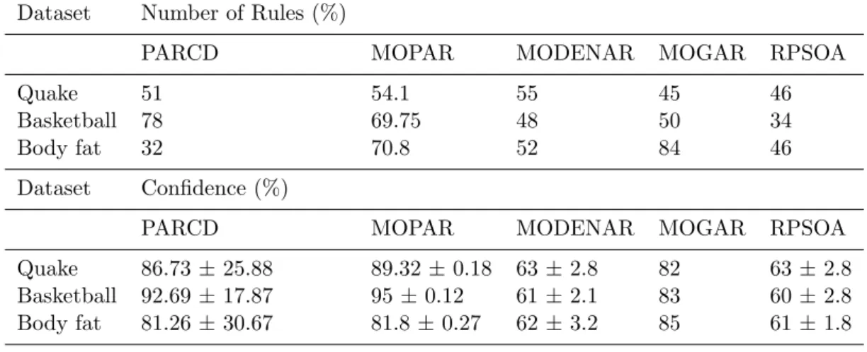
2.11 The comparison of number of rules and confidence values . . . 28
2.12 The comparison of size and Amplitude value . . . . 29
3.1 Parameters . . . . 35
3.2 Representation of Rules . . . . 38
3.3 Number of Matching Rules . . . . 39
5.1 p-value and standard error model . . . . 51
5.2 Parameter of AR model . . . . 51
5.3 Comparison of MAE and MSE . . . . 53
6.1 Testing result . . . . 62
7.1 Coordinate position of observation point and plant of bioelec- tric potential . . . . 71
7.2 Standar error of AR model . . . . 72
7.3 The component of each model . . . . 73
7.4 The Position estimation . . . . 73
Acknowledgements
Thanks to the God. Finally, I could finish for writing this thesis. This thesis comprises some papers from our international proceedings and inter- national journals. This is a final report for completing my doctoral program in Kanazawa University in divison of electrical engineering and computer science, especially from artificial intelligence laboratory.
Let’s me to say thank you so much for my scholarship sponsors. They are Indonesian goverment especially for Minister of Research and Higher Education and Kanazawa University. And also for my institution in Indone- sia, STMIK AMIKOM Purwokerto for supporting my study. Thank you so much for my supervisor, Assoc. Prof. Hidetaka Nambo, who always support, sharing knowledge, supervise, and many more. For my special persons who always give me pray and motivation, my parents, my wife, and my childrens.
In addition, to all of my friends and colleagues who give me advise, help, and suggestion which I do not mentions specifically.
I wish this thesis could be useful for enhancing the insight especially in topic of association analysis. Let’s me know if anytime there is mistake for improving my report. Thank you for everything,
Imam Tahyudin
Kanazawa, June 2018
Chapter 1 Introduction
In Japan, the aging society is the very big problem. In 2014, a publication of the aging society published by the Japanese cabinet office, announced in October 2010 and October 2013 which there are 23% and 25.1% of the elderly population respectively [1]. Their average age is more than 65 years. This condition is the highest proportion in the world [1], [2].
Based on the research of Nomura et al [1], the condition of the elderly is mapped into two groups: the elderly who live with their families and who live alone. Based on data from samples taken in one of the major provinces in Japan, Kyoto, mention that the number of the second group in 1990 are 43.416 (13.3%) then in 2010 has increased by 110.366 (18.2%).
These conditions lead to various problems one of which is the death that do not known by others, whether caused by accidents in their home or other factors such as murder. Based on the same research, the deaths caused by accidents in the home because it was not helped as much as 12.5% [1].
This reality makes the increasing demand of indoor monitoring. One of the measures being initiated is to examine the installation of CCTV cam- eras. This camera can monitor that accidents and immediately helped by a neighbor or an authorized officer. However, this solution does not accept because of privacy concerns. Moreover, the use of infrared sensors tested to solve this problem. Despite of the results were pretty good but it is high cost because it requires many sensor cells [3]. Then, the other solutions have been tried by using the sense of odor but the results are not so good because there are much noisy when the data records [3]. Regarding this problem, we proposed a solution which by using bioelectric potential sensor. This is able to be used for detecting human behavior and friendly to use in private area.
In addition, the cost is achievable.
1.1 Monitoring by Bioelectric Potential of Plant
Plant of bioelectric potential generates a low electrical signal because of the plant activities such as photosynthesis and transpiration. Furthermore, the electrical signal will change because of environmental factors such as temper- ature, humidity and human behavior. The use of bioelectric potential plant could be the solution for monitoring human activities in private area like bath room or bed room. Moreover, it is low cost and it could be a healing media because it produces an oxygen to reduce stress and gives feeling fresh [3], [4], [5], [6], [7].
Based on research Hirobayashi et al [8], states that human activities like stepping around the plants produce a strong correlation with changes the signal by using plant bio-electrical potential. Another study conducted by Nomura et al [4], Shimbo et al [9], explaining that human behavior such as moving, walking, communicating and opening the door can be distinguished using bio electric potential. Furthermore, research conducted by Jin et al [3], utilizing bio electric potential plant to determine the distance of human to the plant by using Artificial Neural Network (ANN). Furthermore, Nambo et al [5]; [6], [7], conducted research to determine the location of one’s position around plant of bioelectric potential. They were using method of classifica- tion, J48 algorithm, multi-layer perceptron (MLP) and deep learning method such as CNN (Convolutional Neural Network).
1.1.1 Measurement of Potential
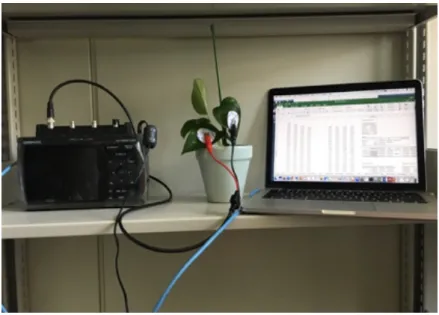
Plant type of this experiment is photos which its leaves are put on two electrodes (figure 1.1). To perform measurements is using a data logger.
Specification of data logger used is GRAPHTEC GL400-4. It measures the low voltage at an average altitude of sampling, 500 Hz. When there is a human activity like walking, the signal is responding on data logger and then the signal results are stored on a PC in real time via the local network (figure 1.2).
1.1.2 The example of signal from Bioelectric Potential of Plant
Figure 1.3 and 1.4 show the output of bioelectric potential plant based on the person existance. In figure 1.3 shows data logger output when no person around the plant and in figure 1.4 when there is a human activity.
The respond of bioelectric potential plant is different, depend on the dis-
Figure 1.1: Experimental design
Figure 1.2: The measurement process
tance. Response is stronger when a person is more near the plant. We can see the differentiation of response signal like the figures 1.5 to 1.6 below [3]:
Therefore, the response of bioelectric potential is proportional to distance.
Base on the experiment if the distance is near so the response is stronger and conversely, if the distance is far (Fig. 1.7) so the response is weaker. In addition, this property can be used for human sensor based on distance [3].
1.2 Research Question (RQ) and Thesis Out- line
The discussion of Bioelectric Potential of plant has been conducted by some
researchers, such as Nomura et al [4], and Shimbo et al [9]. They have been
Figure 1.3: A plant bioelectric potential when no one is near the plant
Figure 1.4: A plant bioelectric potential when a person is stepping near the plant
studied about the implementation of bioelectric potential of plant for detect- ing human behavior such as moving, walking, jumping, and opening the door.
They successfully distinguished those human behavior using bioelectric po-
tential of plant. Furthermore, the successfully research which has conducted
by Jin et al [3] about utilizing bioelectric potential of plant to determine the
distance of human to the plant by using Artificial Neural Network (ANN). In
addition, Nambo et al [5] [6], [7] have been conducted research to determine
the location of resident’s position around plant of bioelectric potential. They
were using method of classification, J48 algorithm, multi-layer perceptron
(MLP) and deep learning method such as CNN (Convolutional Neural Net-
work). The main problem of this research is how to obtain the best accuracy
for solving all cases. Especially, the accuracy to estimate human position
around the bioelectric potential of plant. In this research, we propose a state
of the art for estimating human position from bioelectric potential data set
using association analysis approach. We studied PSO which is developed by
combining with Cauchy distribution. Furthermore, we also conducted re-
Figure 1.5: When the distance is 0.5 m
Figure 1.6: When the distance is 1 m
search using other approach, time series method, as a research comparison.
Therefore, we formulate the following main question to be answered in this thesis.
Main RQ: How can we design, implement and evaluate the best accuracy for estimating human position using bioelectric potential of plant by some approaches. Such as association analysis and time series approaches.
In order to answer this question, we need to address two main approaches.
First, we need to understand about the development of association analy-
sis for numerical data using benchmark data set by combination PSO and
Cauchy distribution (PARCD) method. After that, we discuss the imple-
mentation of association analysis approach for determining human position
using bioelectric potential plant. Second, we perform another approach using
statistical approach, time series model.
Figure 1.7: When the distance is 1.5 m
1.2.1 Part I. Bioelectric potential of plant for estimat- ing human position using association analysis ap- proach
In this part, we study about association analysis and the optimization using combination PSO and Cauchy distribution (PARCD) method. After that, the optimized method is used to determine the position of resident near bio- electric potential of plant. This part is started from Chapter 2, we look at how the concept of combination of evolutionary algorithm method for solving numerical association rule problem by benchmarking dataset. In section 2.2, we look at how the time complexity of A priori and evolutionary algorithm for numerical Association Rule Mining Optimization. In Section 2.4.3, We extract the rule of combination PSO and Cauchy distribution. In Section 2.4.5, We compare the result of optimization improvement of numerical as- sociation rule Mining, PARCD method to other methods. In Chapter 3. We implement the association analysis approach which optimized by PSO to de- termine human position on bioelectric potential dataset (MOPAR) method.
RQ1. How is the Association analysis approach which is optimized using combination evolutionary algorithm in benchmark data set?
RQ2. How is the computational complexity of conventional a priori and evolutionary method?
RQ3. How is to extract the rule determination of proposed method?
RQ4. How does the comparison of PARCD method result with other meth- ods?
RQ5. How is the implementation of association analysis method to overcome
bioelectric potential of plant dataset for determining human location?
1.2.2 Part II. Bioelectric potential of plant for deter- mining human position using time series approach
In part II, we analyze the bioelectric potential of plant for determining hu- man position using time series approach. In this part II starts from chapter 4, we construct the auto regressive (AR) model which is optimized with grid search method. In chapter 5, we compare the result of conventional AR, optimized AR, and MA model. In chapter 6, we build the seasonal ARIMA model using bioelectric potential dataset. In chapter 7, we use AR model to estimate the human position using bioelectric botential dataset. These chapters are centered around the following question:
RQ6. How is to build optimized AR model using benchmark dataset?
RQ7. How does the comparison result for AR, optimized AR, MA, and sea- sonal ARIMA model using bioelectric potential Dataset?
RQ8. How is to use AR model to estimate the human position using bio- electric potential dataset
1.3 Guide for The reader
This thesis is a collection of published papers, either from international con-
ference papers or international journal papers. Each chapter is a paper that
can be read independently from the other chapters. This means that when
reading the thesis as a whole, some repetition is unavoidable. However, since
most chapters cover different topics the redundancy is not large. Therefore,
in order to serve the readers that will not read the entire thesis, we have
chosen to edit the chapters as little as possible.
Part I
Bioelectric Potential of Plant for Determining Human Position using Association
Analysis Approach
Chapter 2
Improved Optimization of Numerical Association Rule Mining by Hybrid PSO and
Cauchy Distribution Approach
2.1 Introduction
The ARM or association analysis method is used to find associations or re- lationships between variables, which often arise simultaneously in a dataset [10]. In other words, association analysis builds a rule for several variables in a dataset that can be distinguished as an antecedent or a consequent. The Apriori and Frequent Pattern (FP) growth methods are widely employed in association analysis. These methods are suitable for categorical or binary data, such as gender data, i.e., males can be represented by 0 and females by 1 [11]. Furthermore, if the data are numeric, such as age, weight or length, these methods process the data by transforming numerical data into categorical data (i.e., a discretization process). This transformation process requires more time and can miss a significant amount of important infor- mation because data transformation does not maintain the main meaning of the original data [12], [13], [14]. For example, if age data represents a 35 years old and is transformed to 1, this obscures the original meaning of the age information. In addition, both methods require manual intervention to determine the minimum support (attribute coverage) and confidence (accu- racy) values. Note that this step is subjective in some cases; thus, the results will not be optimal [15], [16].
To resolve this problem, some researchers have proposed solutions that
employ optimization approaches, e.g., particle swarm optimization (PSO) [13], [17], fuzzzy logic [18] and [19], and genetic algorithm (GA) [12] and [16]. Regarding of the PSO approach which has multiple objective functions for solving association analysis of numerical data without a discretization process. This research produced the better result than other previous opti- mization methods. It has optimum value automatically without determining the minimum support and minimum confidence. However, this method can also become trapped in local optima. When iterations are complete and the number of iterations tends toward infinity, the velocity value of a particle approaches 0 (the weight value of the velocity function is between 0 and 1).
Therefore, the search is terminated because the PSO method can not find the optimal value when the velocity value is 0. Thus, PSO often fails to seek the overall optimal value [15], [16].
We proposed a method that can address the premature searching and the limitations of traditional methods that it does not use a discretization process. In other word, the original data are processed directly using the concept of the Michigan or Pittsburgh approaches. Furthermore, support and confidence threshold values are determined automatically using the Pareto optimality concept. One solution to this problem is by combining PSO with the Cauchy distribution. This combination increases the size of the search space and is expected to produce a better optimal value. Yao et al (1999) reported that combining a function with the Cauchy distribution will result in a wider coverage area; thus, when the Cauchy distribution is combined with the function of the PSO method, the optimal value will increase [20].
Therefore, the purpose of this study is to find the optimal value of the numerical data in association analysis problems by combining PSO with the Cauchy distribution (PARCD). Furthermore, we determine the value of sev- eral objective functions such as support, confidence, comprehensibility, in- terestingness, and amplitude, as a parameter to evaluate the performance of the proposed method.
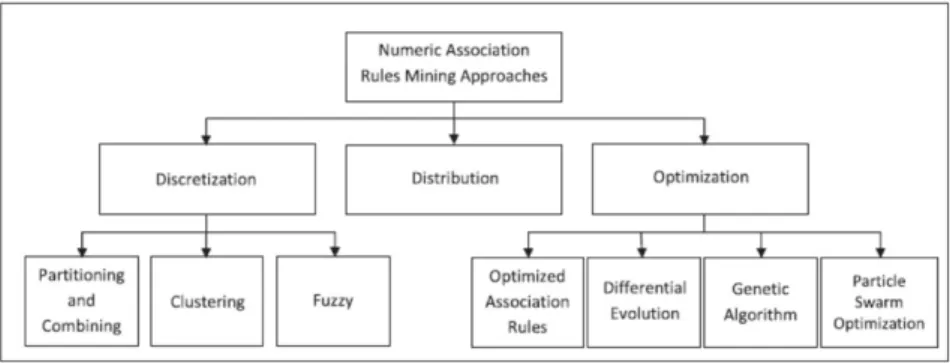
Problem solving in numerical data association analysis is generally per- formed using several approaches, including discretization, distribution and optimization. That the discretization is performed using partitioning and combining, clustering [19], and fuzzy [18] methods, and the optimization approach is solved using the optimized association rule [14], differential evo- lution [21], GA [12], [16], and PSO [13], [17] (Fig. 2.1).
We focus to solve the problem of association analysis of numerical data by
optimization. The previous research from optimization approach is known
as the GAR method. It has been attempted to find the optimal item set
with the best support value without using a discretization process [14]. And
then, the differential evolution optimization approach includes the genera-
Figure 2.1: Numeric Association Analysis Rule Mining
tion of the initial population, as well as mutation, crossover and selection operations. The multi-objective functions are optimized using the Pareto optimality theory. This method is known as MODENAR [21]. Furthermore, a study of numerical association rule mining using the genetic algorithm ap- proach (ARMGA). It successfully solved association analysis of numerical data problems without determining the values of the minimum support or minimum confidence manually. In addition, this method can extract the best rule that has the best relationship between the support and confidence val- ues [16]. Another study of GA approach has been used MOGAR method.
It presented that using MOGAR method was faster than using conventional methods, such as Apriori and FP-growth algorithms, because the time com- plexity of the MOGAR method tends to be simpler, and follows quadratic distribution. On the other hand, the Apriori algorithm follows an exponential distribution, which requires more time for computation [12].
Next, the optimization method has been used PSO for solving numeri-
cal ARM problem. Some authors who performed PSO method such as they
used ARM to investigate the association of frequent and repeated dysfunction
in the production process. The result obtained a faster and more effective
optimization employed PSO, which resulted in a faster and more effective
optimization process than the other optimization methods [22]. In addi-
tion, the PSO approach was used to improved the computational efficiency
of ARM problems such that appropriate support and confidence values could
be determined automatically [23]. In 2012, the development of PSO for ARM
problems was performed by weighting the item set. This weighting is very
important for very large data because such data often contain important in-
formation that appears infrequently. For example, in medical data, if there is
a rule {stiff neck, fever, aversion to light} → {meningitis} that rarely appears
but this rule is very important because in fact this condition is often happen [24]. In 2013, Sarath and Ravi introduced binary PSO (BPSO) to generate association rules in a transaction database. This method is similar to the Apriori and FP growth algorithms; however, BPSO can determine optimum rules without specifying the minimum support and confidence values [25]. In 2014, Beiranvand et al. studied numerical data association analysis using the PSO method. They stated that the employed method could effectively ana- lyze numerical data association analysis problems without using a discretiza- tion process. This research employs four objective functions, i.e., support, confidence, comprehensibility and interestingness. This method is referred to as MOPAR [13]. In 2014, Indira and Kanmani conducted research using a PSO approach; however, they attempted to improve results and analysis time using an adaptive parameter determination process to determine various parameters, such the constant and weight value in a velocity equation. They developed the Apriori algorithm using a PSO approach (APSO), and the results demonstrated that this approach was faster and better compared to using only an Apriori method [17]. In addition, the combination of PSO and GSA has been conducted for solving optimal reactive power dispatch prob- lem in power system. The problem has succesfully accomplished on basis of efficient and reliable technique. And then, the result were found satisfactorily to a large extent that of reported earlier [26]. Verma and Lakhwani exam- ined ARM problems by combining PSO and a GA. The results showed better accuracy and consistency compared to individual PSO or a GA method [27].
There are many developments of PSO method. i.e. the papers about the hybrid method. One of hybrid methods is the hybrid PSO with the Cauchy distribution [28]. This method provides better results compared to using only PSO. In 2011, this combined method was retested for SVM parameter selection [29], [30], [31]. The combined approach was also used to improve performance weaknesses in a process to identify a watermark image based on discrete cosine transform (DCT). The results demonstrated that combining PSO with the Cauchy distribution outperforms the compared method [32]. In 2014, an empirical study demonstrated that combining PSO with the Cauchy distribution provided. The results show that the use of PSO with Cauchy distribution higher than using only PSO [33].
To the best of our knowledge, combining PSO with the Cauchy distri- bution has not been applied to ARM problems that involve numerical data.
This research has important contribution for optimization approach of nu-
merical ARM problem.
2.2 Time Complexity of A priori and Evolu- tionary Algorithm
Nowadays the numerical association rule mining problem is an interesting topic that has been studied using various approaches. Among these are con- ventional methods like Apriori and FP growth [10], [34], [11], discretization approaches like partitioning and combining, clustering and fuzzy [35], [36], by optimization methods like Genetic Algorithms (GA), differential evolution and Particle Swarm Optimization (PSO) [18], [19].
The PSO method is one of the evolutionary algorithms used for solving the ARM problem [13]. However, this method has the drawback that it may become trapped in local optima when the number of iterations goes to infinite then the particle velocity tends to 0. As such, the PSO does not have the capability to search for the optimal solution [37]. This weakness has been solved by combining PSO with Cauchy distribution [38]. This combination can do the searching process faster than traditional methods.
2.2.1 Discussion of Time Complexity
There are some factors which influence to the time complexity of an a priori algorithm. These are the minimum support threshold, the number of items, the number of transactions, the average transaction width, the generation of frequent 1-itemsets, candidate generation and support counting. These factors will be explained in details below: [39]
Minimum Support Threshold
The minimum support threshold often results in more item sets being declared as frequent. This has an adverse effect on the computational com- plexity of the algorithm because more candidate item sets must be generated and counted. The maximum size of frequent item sets also tends to increase with minimum support thresholds. Accordingly, as the maximum size of the frequent item sets increases, the algorithm will need to make more passes over the data set [39].
Number of Items (Dimensionality)
As the number of items increases, more space will be needed to store the support counts of items. If the number of frequent items also grows with the dimensionality of the data, the computation and I/O costs will increase because of the larger number of candidate item sets generated by the algorithm [39].
Number of transaction
Since the a priori algorithm makes repeated passes over the data set, the
run time increase exponentially with a larger number of transactions. But to emphasize it is not a linear increase in processing time [39].
Average transaction width
For dense data sets, the average transaction width can be large. This affects the complexity of the a priori algorithm in two ways. First, the max- imum size of frequent item sets tends to increase as the average transaction width increases. As a result, more candidate item sets must be examined during candidate generation and support counting. Second, as the transac- tion width increases, more item sets are contained in the transaction. This will increase the number of hash tree traversals performed during support counting [39].
Generation of frequent 1-item sets
For each transaction, we need to update the support count for every item present in the transaction. Assuming that w is the average transaction width, this operation requires O(N w) time, where N is the total number of transactions [39].
Candidate generation
To generate candidate k item sets, pairs of frequent (k − 1) item sets are merged to determine whether they have at least (k − 2) items in common.
Each merging operation requires at most (k −2) equality comparisons. In the best-case scenario, every merging step produces a viable candidate k item set.
In the worst-case scenario, the algorithm must merge every pair of frequent (k − 1) item set found in the previous iteration [39].
Support counting
Each transaction of length |t| produces
|t|k
item sets of size k. This is also the effective number of hash tree traversals performed for each transaction.
The cost for support counting is 2.1
O N X
k
(
ωk) α
k!
, (2.1)
where ω is the maximum transaction width and k is the cost for updating the support count of a candidate k-item set in the hash tree [39].
According to the previous researchers, apriori based algorithm based is
slow because increasing the number of attributes results in an exponential
increase of the running time. As depicted in equation 2.2, the computation
complexity of an a priori algorithm follows an exponential distribution. In
this equation, d is the number of attributes and N shows the number of
transactions or records in a data set [13], [12].
T imeComplexity = O(F indingF requentItemSets) + O(RuleGeneration)
= O(N ∗ d ∗ 2
d) + O
d−1
X
k+1
"
d k
∗
d−k
X
j=1
d − k j
#!
= O(N ∗ d ∗ 2
d) + O(3
d− 2
d+1+ 1)
= O(N ∗ d ∗ 2
d) + O(3
d)
= O(2
d+1)
(2.2) Because of the order of the time complexity is exponential, the a priori algorithm runs slowly because as many as the number of attributes used increases, the time complexity is longer.
On the other hand, the time complexity of evolutionary algorithms follows a quadratic distribution O(n
2). Because of the number of iteration is fixed so that the complexity of the algorithm is equal to O(2
d+1) or O(n
2). Lobo et al. and Oliveto et al. explained that it diminishes the relevance of a fixed mutation operator as a means of introducing diversity in the population [40], [41].
2.3 Research Method
2.3.1 The Particle Representation
The rules of numerical association rule mining by PARCD will be obtained by the particle representation procedure. This study used Michigan method which determine for every particle referring to one rule [13]. For wich the data set will be extracted into ACN category, based on the lower and upper bound value. Antecedent is pre- condition and consequent is conclusion for describing a rule. The PARCD method can classify automatically the ACN based on the optimal threshold in every rules. This concept can be showed clearly by Table 2.1.
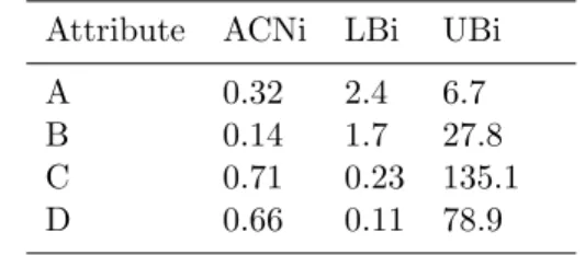
If the optimal procedure for one rule are 0 ≤ ACN i ≤ 0.33 for antecedent,
0.34 ≤ ACN i ≤ 0.66 for consequent and 0.67 ≤ ACN i ≤ 1.00 for none of
them. For instance, see table 2.2. The attribute A and B are the antecedent
and the attribute D is consequent. The attribute C is not appearing because
it not includes both of them. Therefore, the rule is AB → D.
Table 2.1: The rule Extraction Attribute 1 ... Attribute n
ACNi LBi UBi ACNi LBi UBi
Table 2.2: Example of The rule Extraction Attribute ACNi LBi UBi
A 0.32 2.4 6.7
B 0.14 1.7 27.8
C 0.71 0.23 135.1
D 0.66 0.11 78.9
2.3.2 Objective Design
This study uses multiple objective functions, i.e., support, confidence, com- prehensibility, interestingness and amplitude. First, the support criterion de- termines the ratio of transactions for item X to the total transaction (D), i.e., support(X) = X/D. Then, if A is the antecedent of the transaction dataset as a pre-condition then C is consequence as the conclusion of a transaction dataset. The support value if A then C (A → C) is computed as follows:
Support(A ∪ C) = | A ∪ C |
| D | (2.3)
where | A ∪ C | is the number of transaction which contain A and C.
The minimum support value is closely linked to the number of items cov- ered to determine the referenced rule. If the threshold value is low, the sup- port covers many items and vice versa. The support measurement is used to determine the confidence measurement criteria, i.e., the criteria used to mea- sure the quality or accuracy of the rule derived from the total transactions.
Such rules are often developed for each transaction to better demonstrate quality or accuracy. [13]. Confidence can be expressed as follows,
Conf idence(A ∪ C) = Support(A ∪ C)
Support(A) (2.4)
However, these criteria are not guaranteed to produce appropriate rules.
Thus, for a given rule to be considered reliable and to provide overall cov-
erage, the result must also satisfy the comprehensibility and interestingness
criteria. Gosh and Nath (2004), stated that less number of attributes in
antecedent component of a rule show that the rule is comprehensible. The comprehensibility measurement criteria can be expressed as follows:
Comprehensibility(A ∪ C) = log(1+ | C |)
log(1+ | A ∪ C |) (2.5) where | C | is the number of consequence item and | A ∪ C | is the rule number of if A then C (A → C).
Next, the interestingness criteria are used to generate hidden information by extracting some interesting rule or unique rule. This criterion is based on the support value and is expressed as follows:
Interestingness(A ∪ C) =
Supp(A ∪ C) Supp(A)
Supp(A ∪ C) Supp(C)
1 − Supp(A ∪ C)
| D |
(2.6)
The right side of Eq. 2.6 consists of three components. The first com- ponent shows the generation probability of the rule that is based on the antecedent attribute. The second is based on the consequence attributes and the third is based on the total dataset. There is a negative correlation between interestingness and support. When the support value is high, the interestingness value is low because the number of frequent items covered is small [13].
The last criterion is the amplitude interval. The amplitude interval, which is a measure of a minimization function, differs from support, confidence and comprehensibility measures, which are maximization functions. The amplitude interval is expressed as follows:
Amplitude(A ∪ C) = 1 − 1
m Σ(i = 1, m)
u
i− l
imax(A
i) − min(A
i)
(2.7) Here, m is the number of attributes in the item set (| A ∪ C |), u
iand l
iare the upper and lower bounds encoded in the item sets corresponding to attribute i. max(A
i)and min(A
i) are the allowable limits of the intervals corresponding to attribute i. Thus, rules with smaller intervals are intended to be generated [21].
2.3.3 PSO
PSO, which was first introduced by Kennedy and Eberhart (1995), is an
evolutionary method inspired by animal behavior, e.g., flocks of birds, school
of fish, or swarms of bees [42]. PSO begins with a set of random particles.
Then, a search process attempts to find the optimal value by performing an update generation process. During each iteration, each particle is updated by following two best values. The first is the best solution (fitness) achieved to this point. This value is called pBest. The other best value tracked by the swarm particle optimizer is the best value obtained by each particle in the population. The value is called gBest. After finding pBest and gBest, each particle’s velocity and corresponding position are updated [17].
Each particle p in some iteration t has a position x(t) and displacement speed v(t). The finest particles (pBest) and best global positioning (gBest) are stored in memory. The speed and position are updated using Eqs. 2.8 and 2.9, respectively [17].
V
inew= ωV
iold+ C
1rand()(pBest − X
i) + C
2rand()(gBest − X
i) (2.8)
X
inew= X
iold+ V
inew(2.9) Here ω is the inertia weight; V
ioldis the velocity of the ith particle before updating; V
inewis the velocity of the ith particle after updating; X
iis the ith, or current particle; i is the number of particles; rand() is a random number in the range (0, 1); C
1is the cognitive component; C
2is the social component;
pBest is the particle best or local optima in some iterations on every running;
gBest is the global best or global optima in some iterations on every running.
Particle velocities in each dimension are restricted to maximum velocity V
max[43].
2.3.4 Cauchy Distribution
Yao et al. (1999) used a Cauchy distribution to implement a wider mutation scale [20]. A general formula for the probability density function is expressed as follows.
f(x) = 1
sπ(1 + ((x − t)/s)
2) (2.10)
A Cauchy random variable is calculated as follows. For any random
variable X with distribution function F . The random variable Y = F (X)
has a uniform distribution in the range [0,1). Consequently, if F is inverted,
the random variable can use a uniform density to simulate random variable
X because X = F
−1(Y ). Therefore, the cumulative distribution function of
Cauchy distribution is expressed as follows
F (x) = 1
π arctan(x) + 0.5 (2.11) Therefore if
y = 1
π arctan(x) + 0.5 (2.12) by inverting its function, the Cauchy random variable can be expressed as follows
x = tan(π(y − 0.5)) (2.13) This function can be expressed by Eq. 2.14 because y has a uniform distri- bution in the range (0,1]. Thus, we obtain the following,
x = tan(π/2 · rand[0, 1)) (2.14)
2.3.5 PSO for Numerical Association Rule Mining with Cauchy Distribution
PARCD is an extension of the MOPAR methods that combines PSO and the Cauchy distribution to solve problems that occur in the association analysis of numerical data [38]. The goal is to find the optimal value of amateurs and avoid being trapped in local optima. Essentially, this method uses the concept of PSO but modifies the velocity equation by including the Cauchy distribution. The velocity function is expressed as follows,
V
i(t + 1) =ω(t)V
i(t) + C
1rand()(pBest − X
i(t))+
C
2rand()(gBest − X
i(t)) (2.15) The next step is normalization by using V
i(t + 1) value (2.15), which makes the vector length 1. The variant of the Cauchy distribution is infinite and the objective function scales are 1 [20].
U
i(t + 1) = V
i(t + 1)
p V
i1(t + 1)
2+ V
i2(t + 1)
2... + V
iK(t + 1)
2(2.16) The result of the normalization process is multiplied by the Cauchy random variable as follows.
S
i(t + 1) = U
i(t + 1) · tan π
2 · rand[0, 1)
(2.17)
Then, the result of Eq. 2.17 which is a combination of the velocity value and the Cauchy distribution, is used to determine the new position of a particle.
X
i(t + 1) = X
i(t) + S
i(t + 1) (2.18)
2.3.6 PARCD Pseudocode and Flowchart
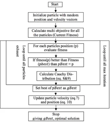
The PARCD pseudocode (Fig. 2.2) and flowchart (Fig. 2.3) show that the algorithm begins by initializing the velocity vector and position randomly.
The algorithm calculates the multi-objective functions as the current fitness.
Then, it executes looping iterations to seek pBest until it finds the gBest value as the optimal solution.
Figure 2.2: PARCD Pseudocode
2.4 Result and Discussion
2.4.1 Experimental Setup
We conducted an experiment using the Quake, Basketball, Body fat, Pollu-
tion, and Bolt benchmark datasets (Table 2.3) from the Bilkent university
Figure 2.3: PSO Flowchart
Table 2.3: Dataset Properties
Dataset No. of Records No. of Attributes
Quake 2178 4
Basketball 96 5
Body fat 252 15
Pollution 60 16
Bolt 40 8
function approximation repository. The experiment was performed using a computer with an Intel Core i5 processor with 8 GB main memory running Windows 7. The algorithms were implemented using MATLAB.
For the proposed algorithm, we set parameter of the population size,
external repository size, number of iterations, C
1and C
2, ω, velocity limit
and xRank (Table 2.4).
Table 2.4: Parameters
Parameter Size External Number of C
1,C
2ω Velocity xRank Repository Size iteration Limit
Average 40 100 2000 2 0.63 3.83 13.33
2.4.2 Experiments
Association rule analysis comprises two steps. The first step is to determine the frequent itemset that includes the antecedents or consequences of each attribute. The second step is to implement the proposed algorithm.
2.4.3 Output Rules of the PARCD Results
This experiment shows the 20
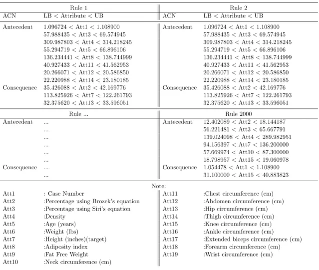
thrun time where each running contains 2000 rules. We presented three datasets of output rules i.e. Body fat, Bolt, and Pollution datasets. Table 2.5 shows the results obtained with the Body fat dataset. For Rule 1, there are eight antecedent attributes and three conse- quent attributes. For Rule 2, the number of antecedent and consequent at- tributes are the same as Rule 1. For the last rule, the number of antecedent and consequent attributes are six and two, respectively.
The antecedent attributes of Rule 1 are case number, percent body fat (Siri’s equation), density, age, adiposity index, chest circumference, abdomen circumference, and thigh circumference. The consequent attributes are per- cent body fat (Brozek’s equation), height, and hip circumference. For Rule 2, the antecedent and consequent attributes are the same as Rule 1. Thus, Rules 1 and 2 can be expressed as follows: if (att1, att3, att4, att5, att8, att11, att12, att14) then (att2, att7, att13). For Rule 2000, the antecedent attributes are Percent body fat using Brozek’s equation, Percent body fat using Siri’s equation, density, height, neck circumference and knee circumfer- ence, and the consequent attributes are case number and weight. Therefore, Rule 2000 is if (att2, att3, att4, att7, att10, att15) then (att1, att6).
Table 2.6 shows the results obtained with the Bolt dataset, which has eight attributes; (run, speed, total, speed2, number2, Sens, time and T20Bolt).
As can be seen, the first two rules the same results for both antecedent and
consequent attributes. The antecedent attributes are total and time, and
the consequent attributes are run and speed1. Therefore, the rule is if (total,
time) then (run, speed1). The rule 2000 shows that the antecedent attributes
are run and speed2. However, the consequent attribute is unknown. Thus,
this rule cannot be declared clearly because it does not have a conclusion.
Table 2.5: ACN Rules of the Body fat dataset
Rule 1 Rule 2
ACN LB<Attribute<UB ACN LB<Attribute<UB Antecedent 1.096724<Att1<1.108900 Antecedent 1.096724<Att1<1.108900
57.988435<Att3<69.574945 57.988435<Att3<69.574945 309.987803<Att4<314.218245 309.987803<Att4<314.218245 55.294719<Att5<66.896106 55.294719<Att5<66.896106 136.234441<Att8<138.744999 136.234441<Att8<138.744999 40.927433<Att11<41.562953 40.927433<Att11<41.562953 20.266071<Att12<20.586850 20.266071<Att12<20.586850 22.220988<Att14<23.180185 22.220988<Att14<23.180185 Consequence 35.426088<Att2<42.169776 Consequence 35.426088<Att2<42.169776
113.825926<Att7<122.261793 113.825926<Att7<122.261793 32.375620<Att13<33.596051 32.375620<Att13<33.596051
Rule ... Rule 2000
Antecedent ... Antecedent 12.402089<Att2<18.144187
... 56.221481<Att3<65.667791
... 139.024098<Att4<289.982951
... 94.156397<Att7<136.200000
... 57.669974<Att10<87.300000
... 18.798957<Att15<19.060978
Consequence ... Consequence 1.054478<Att1<1.108900
... 31.100000<Att15<40.883823
Note:
Att1 : Case Number Att11 :Chest circumference (cm)
Att2 :Percentage using Brozek’s equation Att12 :Abdomen circumference (cm) Att3 :Percentage using Siri’s equation Att13 :Hip circumference (cm)
Att4 :Density Att14 :Thigh circumference (cm)
Att5 :Age (years) Att15 :Knee circumference (cm)
Att6 :Weight (lbs) Att16 :Ankle circumference (cm)
Att7 :Height (inches)(target) Att17 :Extended biceps circumference (cm)
Att8 :Adiposity index Att18 :Forearm circumference (cm)
Att9 :Fat Free Weight Att19 :Wrist circumference (cm)
Att10 :Neck circumference (cm)
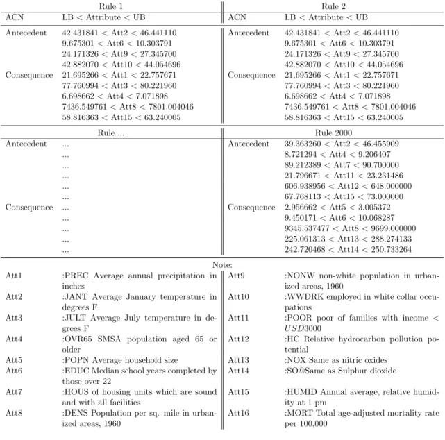
Table 2.7 shows the rule results for the pollution dataset obtained using the proposed particle representation PARCD method. The results for the first and second rules are the same. Here, the antecedent attributes are JANT, EDUC, NONW, and WWDRK, and the consequent attributes are PREC, JULT, OVR65, DENS and HUMID. Thus, the rule is if (JANT, EDUC, NONW, WWDRK) then (PREC, JULT, OVR65, DENS, HUMID).
The Rule 2000 has an ACN result that differs from the first and sec-
ond attributes. The antecedent attributes of Rule 2000 are JANT, OVR65,
HOUS, POOR, HC and HUMID and its consequent attributes are POPN,
EDUC, DENS, NOX, and SO@. Thus, the final rule is if (JANT, OVR65,
HOUS, POOR, HC) then (POPN, EDUC, DENS, NOX, SO@).
Table 2.6: ACN Rules of the Bolt dataset Rules ACN LB < Attribute < UB
Rule 1 Antecedent 11.911616 < Att3 < 16.259242 62.782669 < Att7 < 65.562550 Consequence 23.688468 < Att1 < 31.295955
5.928943 < Att2 < 6.000000 Rule 2 Antecedent 11.911616 < Att3 < 16.259242
62.782669 < Att7 < 65.562550 Consequence 23.688468 < Att1 < 31.295955
5.928943 < Att2 < 6.000000 ...
...
Rule 2000 Antecedent 13.621221 < Att1 < 29.817232 1.761097 < Att4 < 2.325029 Consequence None
Note :
Att1 :RUN
Att2 :SPEED1
Att3 :TOTAL
Att4 :SPEED2
Att5 :NUMBER2
Att6 :SENS
Att7 :TIME
Att8 :T20BOLT
2.4.4 Output of multi-objective function and correla- tion of PARCD methods
The basic concept of association analysis comprises two steps, i.e., the first step is the determination rules which in every rule contain antecedent and consequent and the second step is the implementation of the algorithm (i.e., the proposed method). This method begins with the initialization process, which as the start of the algorithm starts with the determine the multi- objective function value and calculates the particle velocity and positioning at i. Then, an iterative process is performed to search for pBest and gBest as the optimal solution.
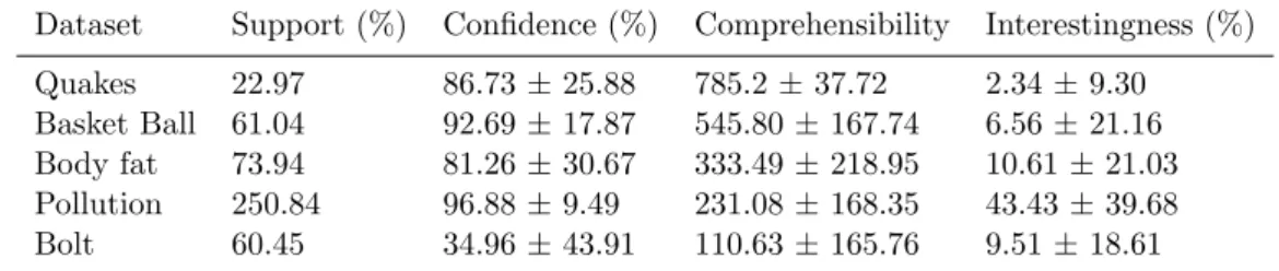
Table 2.8 shows the results of the multi-objective function of the PARCD
method. Here, there are four parameters i.e., support, confidence, compre-
hensibility and interestingness. Then, the method is examined using five
Table 2.7: ACN Rules of the Pollution dataset
Rule 1 Rule 2
ACN LB<Attribute<UB ACN LB<Attribute<UB Antecedent 42.431841<Att2<46.441110 Antecedent 42.431841<Att2<46.441110
9.675301<Att6<10.303791 9.675301<Att6<10.303791 24.171326<Att9<27.345700 24.171326<Att9<27.345700 42.882070<Att10<44.054696 42.882070<Att10<44.054696 Consequence 21.695266<Att1<22.757671 Consequence 21.695266<Att1<22.757671
77.760994<Att3<80.221960 77.760994<Att3<80.221960 6.698662<Att4<7.071898 6.698662<Att4<7.071898 7436.549761<Att8<7801.004046 7436.549761<Att8<7801.004046 58.816363<Att15<63.240005 58.816363<Att15<63.240005
Rule ... Rule 2000
Antecedent ... Antecedent 39.363260<Att2<46.455909
... 8.721294<Att4<9.206407
... 89.212389<Att7<90.700000
... 21.796671<Att11<23.231486
... 606.938956<Att12<648.000000
... 67.768113<Att15<73.000000
Consequence ... Consequence 2.956662<Att5<3.005372
... 9.450171<Att6<10.068287
... 9345.537477<Att8<9699.000000
... 225.061313<Att13<288.274133
... 242.720468<Att14<250.733264
Note:
Att1 :PREC Average annual precipitation in inches
Att9 :NONW non-white population in urban- ized areas, 1960
Att2 :JANT Average January temperature in degrees F
Att10 :WWDRK employed in white collar occu- pations
Att3 :JULT Average July temperature in de- grees F
Att11 :POOR poor of families with income <
U SD3000 Att4 :OVR65 SMSA population aged 65 or
older
Att12 :HC Relative hydrocarbon pollution po- tential
Att5 :POPN Average household size Att13 :NOX Same as nitric oxides Att6 :EDUC Median school years completed by
those over 22
Att14 :SO@Same as Sulphur dioxide Att7 :HOUS of housing units which are sound
and with all facilities
Att15 :HUMID Annual average, relative humid- ity at 1 pm
Att8 :DENS Population per sq. mile in urban- ized areas, 1960
Att16 :MORT Total age-adjusted mortality rate per 100,000
datasets i.e., quake, basketball, body fat, bolt, and pollution. Generally, the Bolt dataset is the dominant data set and has the highest value for each pa- rameter (except comprehensibility). Conversely, the least dominant dataset is quake (with the exception of the confidence parameter).
The first parameter, i.e., support, showed a higher value with the Bolt
dataset (250.84%) and the lowest with the quake dataset (22.97%). The
average was approximately 90%. The highest confidence value was similar
Table 2.8: The output of PARCD method
Dataset Support (%) Confidence (%) Comprehensibility Interestingness (%) Quakes 22.97 86.73 ± 25.88 785.2 ± 37.72 2.34 ± 9.30
Basket Ball 61.04 92.69 ± 17.87 545.80 ± 167.74 6.56 ± 21.16 Body fat 73.94 81.26 ± 30.67 333.49 ± 218.95 10.61 ± 21.03 Pollution 250.84 96.88 ± 9.49 231.08 ± 168.35 43.43 ± 39.68 Bolt 60.45 34.96 ± 43.91 110.63 ± 165.76 9.51 ± 18.61
to the support value. The highest confidence value was obtained with the Bolt dataset (96.88%) with a deviation of approximately 10. The lowest confidence value was obtained with the pollution dataset (34.96%) with a very high deviation of just under 45. The average confidence value was ap- proximately 80%. The highest comprehensibility value was obtained with the Quake dataset (approximately 785). The lowest comprehensibility value was obtained with the pollution dataset (approximately 110 with a devia- tion, well over 165). The average comprehensibility value was approximately 400. The final parameter, i.e., interestingness, obtained the highest value with the bolt dataset (approximately 43% with a deviation of just under 40). The lowest interestingness value was obtained with the quake dataset (2.34% with a deviation of just under 10). The average interestingness value was approximately 15%. This demonstrates that the support and confidence values, i.e., 90% and 80% respectively, were satisfactory. Moreover, the com- prehensibility value was four times better; however, the interestingness value was not satisfactory (approximately 15%).
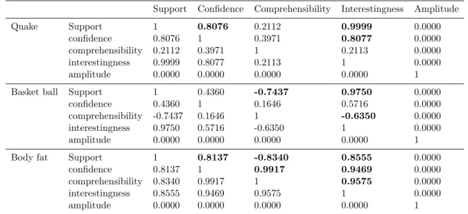
The correlation values between each objective function are shown in Table 2.9 and Figure 2.4. The results show one objective function with another are significant association either be positive or negative. The correlation value of all objective functions to amplitude was always close to zero. In other words, the correlation to the amplitude function was low. This proves the opinion given by Alatas et al. (2008), i.e., the amplitude function differs from other functions because it attempts to minimize while the other functions attempt to maximize their values.
2.4.5 The comparison of multiobjective function be- tween PARCD and other methods
Table 2.10 shows a comparison of the support value obtained by the proposed
PARCD method and five previous methods (i.e., the MOPAR, MODENAR,
Table 2.9: Correlation of multi-objective function
Support Confidence Comprehensibility Interestingness Amplitude
Quake Support 1 0.8076 0.2112 0.9999 0.0000
confidence 0.8076 1 0.3971 0.8077 0.0000
comprehensibility 0.2112 0.3971 1 0.2113 0.0000
interestingness 0.9999 0.8077 0.2113 1 0.0000
amplitude 0.0000 0.0000 0.0000 0.0000 1
Basket ball Support 1 0.4360 -0.7437 0.9750 0.0000
confidence 0.4360 1 0.1646 0.5716 0.0000
comprehensibility -0.7437 0.1646 1 -0.6350 0.0000
interestingness 0.9750 0.5716 -0.6350 1 0.0000
amplitude 0.0000 0.0000 0.0000 0.0000 1
Body fat Support 1 0.8137 -0.8340 0.8555 0.0000
confidence 0.8137 1 0.9917 0.9469 0.0000
comprehensibility 0.8340 0.9917 1 0.9575 0.0000
interestingness 0.8555 0.9469 0.9575 1 0.0000
amplitude 0.0000 0.0000 0.0000 0.0000 1