57
International review for spatial planning and sustainable development, Vol.3 No.4 (2015), 57-74 ISSN: 2187-3666 (online)
DOI: http://dx.doi.org/10.14246/irspsd.3.4_57
Copyright@SPSD Press from 2010, SPSD Press, Kanazawa
A Spatial Simulation Model to Explore Agglutination of Residential Areas and Public Service Facilities
Kazuki Karashima
1*, Akira Ohgai
1and Atsushi Motose
11 Department of Architecture and Civil Engineering, Toyohashi University of Technology
* Corresponding Author, Email: [email protected] Received 21 July, 2014; Accepted 10 March, 2015
Key words: Spatial Agglutination, Residential Areas, Public Service Facilities, Multi-agent based Model, Simulation
Abstract: According to a 2006 report by the National Institute of Population and Social Security Research, Japan has been undergoing a long-term decline in population since 2005. The mid-term and long-term vision of urban and regional planning regards the consolidation of residential areas and public service facilities, including their withdrawal, as necessary for improving the quality of life for rural and suburban residents. From the point of view of provider’s such as the administrative and private sectors, consolidation of facilities is inevitable due to their profitability. Because of the decrease in the number of facility users and their lack of successors, brought about by population decline and aging, it is also difficult for the public administration to provide public services. The purpose of this study is to produce suggestions for sustainable urban and regional spatial structures in Japan. A spatial simulation model was used as a multi-agent-based model to analyze the mid- and long-term changes in the agglutination of residential areas and public service facilities. At first, a multi-agent-based model was developed to quantitatively evaluate the agglutination of residential areas and public service facilities. Next, sensitivity analysis was conducted to adjust some of the crucial parameters that influenced simulation results. Finally, simulations were carried out based on several policy scenarios related to the sustainability and accessibility of the facilities. The results of the analysis indicated that public service facilities are likely to be concentrated in the city center, but that financial support by the administration or non-profitable organizations (NPO) enables facilities located outside of centers to sustain the provision of public service.
1. INTRODUCTION
1.1 Background and Purpose
According to a 2006 report by the National Institute of Population and
Social Security Research, Japan has been undergoing a long-term decline in
population since 2005. As a result of the population decline, decreasing birth
rate and aging population, it would be difficult for local residents to
sustainably receive the primary services that are necessary for daily life (for
example, medical, sales, financial services, etc.) because the mid-term and
long-term vision of urban and regional planning considers the consolidation
of residential areas and public service facilities, including their withdrawal,
as necessary to improve quality of life for rural area and suburban residents.
In addition, from the point of view of provider, such as the administration and private sectors, the consolidation of the facilities is inevitable due to their profitability. Because of the decrease in the number of facility-users and their lack of successors caused by population decline and aging, it is also difficult for the public administration to provide public services.
The purpose of this study is to produce suggestions for sustainable urban and regional spatial structures in Japan. A multi-agent-based spatial simulation model is used for analyzing the mid- and long-term locational changes in residential areas and service facilities.
1.2 Related Studies
At present, sustainability is a popular term. It is often used in the context of global environmental issues, for example, greenhouse gases, in referring to climate change and energy problems. In the field of urban planning, one of the concepts for creating a sustainable urban form, that is, a “compact city,” is widely spreading. For example, Jenks et al. (1996) describe the concept of compact cities. This concept is reflected in many policies and practices globally.
In recent years, some countries, including Japan, have faced long-term depopulation as a sustainability issue. Many researchers have focused on the issue of urban shrinkage, a multidimensional phenomenon encompassing regions, cities and parts of cities or metropolitan areas that are experiencing population loss and a dramatic decline in their economic and social base. For example, Pallagst et al. (2014) and Richardson and Nam (2014) describe the concept of the shrinking city. A recent international debate on urban shrinkage has ensued due to the enhanced scholarly understanding of urban shrinkage, which reflects governance and policy. For example, Großmann et al. (2013) organized various studies related to urban shrinkage to augment and improve the international urban shrinkage research agenda. Rall and Haase (2011) evaluated the utility of a program in Leipzig, an example of a shrinking city that began to revitalize its declining neighborhoods. Kabisch and Grossmann (2013) focused on how a declining and aging population impacts the population composition within a particular estate, how residential satisfaction in the estate changed over time, and which target groups are attracted to the estates, using the results from a unique long-term sociological survey that was carried out for over 30 years in a large housing estate in Leipzig, eastern Germany. Schetke and Haase (2008) developed and applied a multi-criteria assessment scheme (MCA) to assess the socio- environmental impact of shrinkage. Frazier et al. (2013) examined the association between building demolition and crime, a human-environment interaction that is fostered by the presence of vacant and abandoned properties, through a comparative statistical analysis.
While studies that clarify the issue of urban planning and the actual conditions such as those mentioned above, are accumulating, exploring the vision and urban structure that corresponds to the issue is essential.
Therefore, studies that explore the vision and urban structure through the use of spatial simulation techniques are also essential.
A review of prior studies regarding spatial simulation demonstrates that
there are various methods of simulating a virtual urban structure. For
example, Gonzales et al. (2013) used a decision-support system (DSS) that
systematically integrates urban metabolism components into impact
assessment processes with the aim of accurately quantifying the potential
effects of difficult proposed planning interventions. Xu and Coors (2012) developed the integration of GIS, SD models and 3D visualization, called the GISSD system, which can better explain the interaction and variation between residential development sustainability indicators. Barredo et al.
(2003) asserted that one of the most potentially useful applications of cellular automata (CA) from the point of view of spatial planning is their use in simulations of urban growth at the local and regional levels. Lagarias (2012) proposed a CA-based model linking macro-scale processes to micro- dynamics to simulate the urban sprawl process.
One of the most popular methods is the multi-agent system (MAS).
Uhrmacher and Weyns (2009) described how MAS has been used to understand the interaction both among agents and between agents and their dynamic environment. For example, Ligtenberg et al. (2004) demonstrated a MAS that consists of agents representing organizations and interest groups involved in an urban allocation problem during a land use planning process.
Ligtenberg et al. (2001) also described a spatial planning model combining a multi-agent simulation (MAS) approach with cellular automata (CA). Tian et al. (2011) developed an agent-based model of urban growth for the Phoenix metropolitan region in the United States, which simulates the behavior of regional authorities, real estate developers, residents, and environmentalists.
Among the studies that focus on the exploration of sustainable urban forms, one example is Zellner et al. (2008), who developed a simple agent- based model of a hypothetical urbanizing area that integrates data on spatial economic and policy decisions, energy and fuel use, and air pollution emissions and assimilation to test how residential and policy decisions affect urban forms, consumption and pollution. To assess the sustainability of urban area socio-ecological systems, Gaube and Remesch (2013) developed an agent-based decision model to simulate new residential patterns for different household types based on demographic development and migration scenarios. Cavari et al. (2011) developed a model to understand and draw conclusions concerning a planner's options in developing a plan that reflects a sustainable built environment in terms of transportation, distribution of facilities and minimization of pollution from vehicles.
Other studies focused on the exploration of the urban form as it corresponds to long-term depopulation. For example, Haase et al. (2012) demonstrated that a selective demolition of the vacant housing stock in Leipzig could counteract the vast supply of dwellings and balance the demand for housing with the number of available flats. He employed the spatially explicit simulation model RESMOBcity. Haase et al. (2012) also provided the initial results of a joint SD (system dynamics)-CA (cellular automata) model and an ABM (agent-based model), both of which operationalized social science data regarding urban shrinkage, using Leipzig, Germany, as a case study.
This paper is unique because it attempts the simulation of future trends of
assumed urban shrinkage focusing on residential areas and public service
facilities to obtain suggestions for creating sustainable urban and regional
structures.
Figure 1. Conceptual diagram of virtual space
■: A facility providing services to the
entire virtual space
■: Neighborhood-oriented facilities
■: Residential area
●: Household
1.3 Study Method
The study procedure is as follows.
First, a spatial simulation model is developed using multi-agent-based modeling. We define service facilities and households as agents. The service facility agents perform withdrawal (agglutination), and the household agents use the facilities and relocate their residences.
Second, sensitivity analysis is conducted to extract the crucial parameters that influence the agglutination of residential areas and service facilities.
Third, based on the results mentioned above, simulations are carried out to simulate policy scenarios related to the sustenance and accessibility of the facilities. Finally, we analyze the results and examine the potential suggestions for sustainable spatial structure in the future.
2. MODEL DEVELOPMENT 2.1 Virtual Spatial Model
The multi-agent-based model is a useful technique for analysing unexpected phenomena. It can show the effects of an individual agent’s activities or the interactions between agents and their environment. With this model, users can demonstrate dynamic and complex changes in an urban or regional area. This type of model is very useful for visually expressing the changes that occur in urban and regional areas over time.
In this paper, a spatial simulation model was developed in order to quantitatively evaluate the agglutination of residential areas and service facilities. This model contains a
hierarchical system of service facility agents and household agents. These agents are generated in a virtual space consisting of grid cells under certain conditions.
The virtual space is composed of grid cells where one cell is defined as a community (village) which roughly equals 1km
2of “real space”. The virtual space contains 441 (21 x 21) cells in total. This virtual space is a closed space with no socio-economic interaction with external forces, such as migration. Statistical data taken from Japan were used. One step in the simulation is equal to one year and lasts for 100 steps, starting in 2005 and ending in 2105.
2.2 Facility Agent
The facility agents are classified into two types; a facility which provides service to the entire virtual space and those that are neighbourhood oriented.
The former is placed in the center of the virtual space, where it represents a
central area in a real world region. The neighborhood-oriented facilities are
randomly allocated throughout the virtual space before the initiation of the simulation. The facilities (agents) choose withdrawal (extinction) by comparing the number of users (households) present during the previous step to the minimum number of users needed for the facility to maintain service.
If the number of users is lower than the requirement, the facility will either withdraw or combine with another facility. This process is based on the idea that the loss of sustainable service, as a result of declining users, can result in the withdrawal or agglutination of a facility.
2.3 Residential Area Agent
Residential area agents are placed in each of the 441 cells, which have variables indicating the maximum number of households that can occupy a cell (MHC), land price, the number of residents, and the number of households. Each cell is randomly assigned an MHC value between 1 and 20 before the simulation’s initiation. The distribution of MHC values mirrors the different distributions of population density found in the real world.
The land price of a cell is determined by the cell’s population density and the attractiveness and accessibility of the nearest facility. A regression analysis using formulas (1) and (2) was conducted using data on land prices from Toyohashi city. A multiple correlation coefficient was given the highest value when β=0.8 and the value of the constant term=0. In this model, we adopt a=271.3, b=7.7, and β=0.8 when the multiple correlation coefficient is the highest.
y
i= ax
1i+ bx
2i(1) x
2i= D
jexp(-βC
ij) (2)
Where y
iis the land price of cell i, x
1iis the population density, x
2iis the convenience of the facilities, D
jis the attractiveness of the nearest facility j (determined by the number of users in the previous step), β is a parameter of the distance decay function, a and b are parameters and C
ijis the distance from cell i to the nearest facility j.
Every facility is given the same initial value for attractiveness.
2.4 Household Agent
The household agents are initially placed at random within the virtual space. Each household agent has four attributes; household type, age, income and house type. The household agent can decide which facility to use and can also decide to relocate to any other cell. The choice of whether to relocate is based on the distance to the nearest facility, the number of neighboring households in the current cell and the head of the household’s age. When relocating to any other cell, the household agent decides on a new residential cell based on the new cell’s land price, their income and the distance from the new cell to the nearest facility. However, the number of households that can relocate to any given cell is limited by the cell’s MHC.
2.4.1 Attributes (1) Household type
We defined household type as being one of the following three types:
single-resident, couple, or couple with 1-3 children. In Japan, approximately
90% of households are either nuclear families or single residents, with
households having more than four children making up less than 10% of the population. Therefore, the household agent assumes a maximum of three children. The ratio of household types was set based on a comprehensive survey on living conditions conducted by the Ministry of Health, Labor and Welfare (MHLW) (2005a).
(2) Ages of the household members
The ages of the household members are stochastically assigned by applying the age structure values of Japan. The population of the age structure was set based on an annual report on population estimates conducted by the Ministry of Internal Affairs and Communications (MIAC) (2005a).
(3) Income
The income of a household agent is stochastically assigned using the ratio between income and the head of the household’s age in Japanese households. The data for this ratio is based on a national survey on family income and expenditure conducted by the MIAC (2004). In the simulation, the income of a household increases at a constant ratio each step as the head of the household ages.
(4) House type
We defined two house types: owner-occupied and rental. The housing type of a household agent was stochastically assigned using the ratio between the housing type and the head of the household’s age. The data for this ratio is based on the housing and land survey conducted by the MIAC (2003).
2.4.2 Change of a Household Agent (1) Generation
When a household agent’s child reaches 20 years of age, that child becomes an independent household agent. Constant responsibility and authority are given to children when they reach 20 years of age in the real world, so the model assumes that children become adult household agents at the age of 20.
(2) Marriage
Based on a national census conducted by the Statistics Bureau of MIAC (2005b), marriage is stochastically assigned to each independent household agent between 20 and 49 years of age. If the age of a male agent is near that of a female agent, female agent’s age is added to an attribute of the male agent and the female agent disappears, indicating a marriage. In addition, it is statistically likely that a bachelor older than 50 years old will be a bachelor for life. Therefore, this model assumes that unmarried agents older than 50 will not marry.
(3) Birth
A newborn child is added to the household agents when the wife of a coupled household agent reaches 20 to 39 years of age, in accordance with the birth rate calculated at the beginning of each step. The number of births is estimated using a cohort model.
(4) Death
The death of a person in a household agent is probabilistically assigned
using the death rate and person’s age at the end of each step. The death rate
by age is based on a monthly report on an outline of vital statistics conducted
by the MHLW (2005b).
Figure 2. Conceptual diagramof P
32.4.3 Choice of a Service Facility
The determination of which service facility a household agent would use was carried out by using the spatial interaction model shown in equation (3).
exp
∑ exp 3
Where P
ijis the probability that a household agent from cell i uses facility j, D
jis the attractiveness of facility j (determined by the number of users in the previous step), C
ijis the distance from cell i to facility j and β is a distance decay parameter.
Every facility is given an equal level of attractiveness at the first step.
2.4.4 Choice of Relocation by a Household Agent
In this model, the probability that a household agent would relocate to any other place (cell) is calculated using the three elements below. (A critical assumption for calibrating this probability is that residents generally have a strong intention to settle in a given location.)
(1) Distance to the facility
This is the distance between the cell a household agent currently lives in and the facility that the agent uses. The probability of relocation due to distance (P
1) is determined using equation (4). This means that the desire to relocate becomes stronger as the distance to the facility becomes farther.
4
α
1: coefficient (arbitrary value)
(2) The number of household agents in the neighborhood
The probability of relocation, due to the number of household agents in the neighborhood (P
2), is determined by equation (5). When the number of household agents in the neighborhood (N) is lower than the minimum number of neighboring households (a), the probability takes on a value greater than 0. The neighborhood is defined as the cells adjacent to the one in question.
,
0, 5
α
2, β
2: coefficients (arbitrary values) (3) Age
The third probability (P
3) is determined by the head of the household’s age as shown in Figure 2.
This is based on Japanese lifestyle trends. Because heads of households that are between 20 and 30 years old can be regarded as having a higher possibility to relocate than any other age group, the value of P
3was set the highest among all age groups
for 20-30 year olds. Conversely, elderly residents have a strong desire to
remain at their current place of residence. Therefore, agents over 70 years
old were given the lowest probability to relocate.
2.4.5 Probability of Relocation
Considering some factors that can affect relocation, apart from the three elements mentioned above, we introduced a stochastic disturbance term (v) in the probability calculation for relocation P. As shown in equation (6), the value of v takes approximately 1 for random numbers (rand) from 0-1 while n takes approximately 0-0.5. Therefore, this disturbance term does not have a large effect on the influence of the three main elements. In addition, the individual difference between the influences from other elements is determined by providing a random number to each household agent. As a result, the probability of relocation P is calculated using equation (7).
Household agents choose whether to relocate to any other place (cell) by using this equation.
ln 6
⁄ 7 2
2.4.6 Choice of a New Address
Once a household agent decides to relocate, they must choose between a new cell where a desired facility is located or a cell neighboring that facility which is as close as possible to the cell where they currently live. The choice of a new address is based on socio-economic conditions. It was assumed that a household agent could relocate to a new cell if the head of the household’s income exceeded the minimum standard allowing him/her to either purchase or rent housing, so long as the population density of the new cell is lower than its MHC. If neither condition mentioned above is satisfied, the household agent will search other cells until they can find a new cell satisfying the necessary conditions.
(1) Purchase of a house
It is assumed that if the cost of purchasing a house at a new address (cell) is less than five times the household agent’s income, then that household agent can relocate to the cell of its choice. In the real world, almost all heads of households receive loans to purchase a house. Generally, a person receives a housing loan that is lower than five times their income. Therefore, using equation (8), we define the condition in which an agent can purchase a house. The house site area was fixed at 170 square meters, which is the average in Toyohashi City. The construction cost was set at 0.5 million yen per 3.3 square meters and the total floor area was set at 120 square meters.
(5 times income) ≧ (land price at a cell *170 m
2+ 0.5 million yen * 120 m
2/3.3m
2) (8) (2) Rental housing
When the annual rental price of a house at a new address (cell) is less than 30% of a household head’s income, a household agent can relocate to that cell using equation (9). One method of real estate appraisal is used as the estimation method for annual rent. Generally speaking, the average annual rent in Japan is less than 30% of a renter’s income. Therefore, the limit on the annual rent of a house was set below 30% of an agent’s income. The area of a rental house was set at 50 square meters, which is the average in Toyohashi City . The construction cost was set at 0.5 million yen per 3.3 square meters and the capitalization rate was set at the net yield, which is generally 6-8%. The annual maintenance cost was set at 120,000 yen.
(30% of income) ≧ (land prices at a cell * 50 m
2+ 0.5 million yen * 50 m
2/3.3m
2) * net yield + 120,000 yen (9)
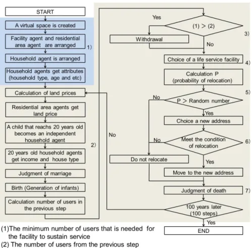
2.5 Simulation Flow
The simulation flow is as follows (Figure 3). Step 1 is the initial setting of the simulation. Steps 2-7 represent the flow for one year, and these steps
are repeated 100 times to quantitatively evaluate the agglutination of residential areas and service facilities over a 100 year period.
In Step 1, a virtual space is created in accordance with the concepts mentioned in Section 2.1. Facility agents, residential area agents and household agents are arranged within the virtual space. Each household agent is then randomly assigned attributes (household type, household member ages, income, and house type).
In Step 2, each residential area agent is given a land price, and the attributes of each household agent are then changed. According to the change, each household agent undergoes generation, marriage, birth and death based on the concepts mentioned in Sections 2.2 - 2.4(1).
In Step 3, facility agents choose whether or not to withdrawal by comparing the number of users (households) in the previous step with the minimum number of users needed for the facility to sustain service based on the concepts mentioned in Section 2.2.
In Step 4, each household agent chooses a service facility by using a spatial interaction model, based on the concepts mentioned in Section 2.4 (4).
In Step 5, the household agents judge whether to relocate.
Figure 3. Simulation flow
In Step 6, household agents that decide to relocate, choose a new cell where there is either a desired facility located or one of its neighboring cells is as close as possible to their cell of origin.
In Step 7, the mortality rate is used to calculate the household agents most likely to die.
3. SENSITIVITY ANALYSIS 3.1 Analysis Method
The following four elements are defined as indices for analyzing the results of the simulation.
(1) Total distance to facilities
This value shows the total travel distance between the cell a household agent lives in and the facility that the household agent uses in each step.
(2) Number of facilities
This value shows the number of facility that provide services to the entire simulation area and the number of neighborhood-oriented facilities in each step.
(3) Residential area ratio
This value shows the ratio between the number of cells in which a household agent is living and the total number of cells in each step.
(4) Compact degree
This value shows the ratio between the number of cells where a household agent currently lives and the number of facilities in each step. A smaller compact degree value indicates that a more compact urban structure is formed.
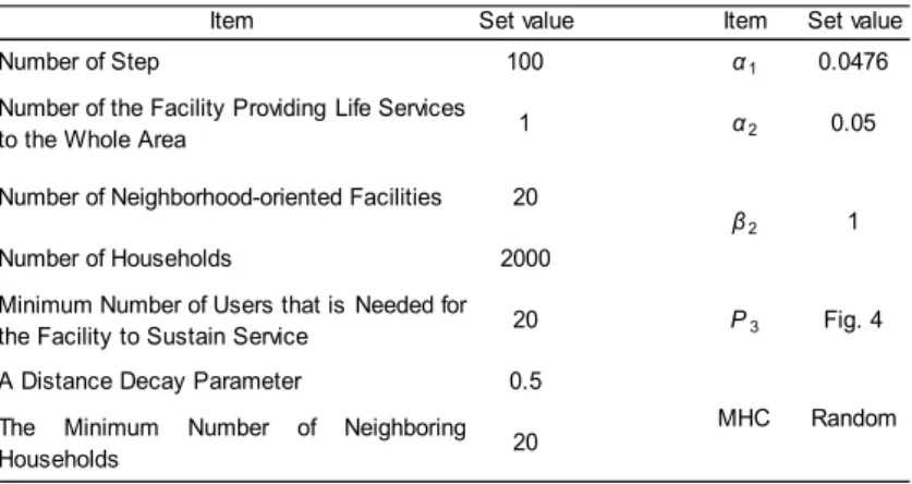
3.2 Parameter Setting
The average relocation rate after 10 full simulations was 4.46%. This value is approximately equal to the 4.45% relocation rate found in the report on internal migration conducted by the MIAC (2005c). Therefore, the values in Table 1 were used for the base case of this model.
Item Set value Item Set value
Number of Step 100
α10.0476
Number of the Facility Providing Life Services
to the Whole Area 1
α20.05
Number of Neighborhood-oriented Facilities 20
Number of Households 2000
Minimum Number of Users that is Needed for
the Facility to Sustain Service 20
P3Fig. 4
A Distance Decay Parameter 0.5 The Minimum Number of Neighboring
Households 20 MHC Random
β2
1
Table 1. Base case
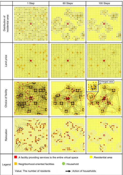
3.3 Simulation Result Using the Base Case
The results of the simulation using the base case are shown in Figure 5 and lead to the following observations.
The agglutination of residential areas arose from cells that were more than 4km from the nearest facility. The land prices around a facility that had many users were higher than those around a facility with few users. In addition, land prices in a cell became cheaper when the distance between two facilities was short because of the dispersion of the residents and users.
Household agents tended to choose the facility nearest to their cell of origin.
Facilities that were close to other facilities and facilities located in the suburbs tended to withdraw. In the case of the former, household agents that lived around the facility tended to relocate to the cells around the more attractive facility.
Figure 5. Simulation result
1 Step 60 Steps 100 Steps
Distribution of residential area Land priceChoice of facilityRelocation
Legend
■
: A facility providing services to the entire virtual space■
: Neighborhood-oriented facilities■
: Residential area●
: HouseholdValue: The number of residents : Action of households
Enlarged view
α1 a α2 Age 2 β 4
P1: Low case1 0.0286
P1: Slightly Low case2 0.0357
P1: High case3 0.0714
P2: High case4 30 0.0333
P2: Slightly Low case5 10 0.1
P2: Low case6 5 0.2
P3: High case7 Fig. 4
P3: Slightly Low case8 Fig. 4
P3: Low case9 Fig. 4
Extremely easy case10 5
Easy case11 10
Slightly difficult case12 30
Difficult case13 40
Extremely difficult case14 80
Extremely easy case15 0.1
Easy case16 0.3
Difficult case17 0.8
Extremely difficult case18 1.0
Low case19 10
Slightly high case20 30
High case21 40
5 MHC-fixting Central area: high
Suburban area: low case22
6
Restricting Placement of Elderly Person.
Central area: high Suburban area: low Edge: high
case23 2
Minimum Number of Users that is
Needed for the Facility to Sustain Service
3
A Distance Decay Parameter
(Accessibility)
4 Number of Facilities
Item Changed value
1
Distance to Facilities The Minimum
Number of Neighboring Households
Age
3.4 Sensitivity Analysis
A sensitivity analysis of the parameters influencing the results of the simulation was performed using the base case. The following six scenarios were analyzed. 1) A scenario where the P
1, P
2and P
3, which influence P (the probability that a household agent relocates to any other cell), are changed.
2) A scenario in which the minimum number of users needed for the facility to sustain service, which affects the withdrawal of facilities, is changed. 3) A scenario in which the parameter of the distance decay function β, which influences the household agent’s facility choice, is changed. 4) A scenario in which the number of facilities is changed. 5) A scenario in which the MHC is fixed. 6) A scenario in which the placement of elderly residents is restricted.
The values in Table 2 show which values changed compared to the base
Figure 4. Relations between Age and P
3Table 2.The changed values from base case (The blank means same value as a base case)
case in each scenario.
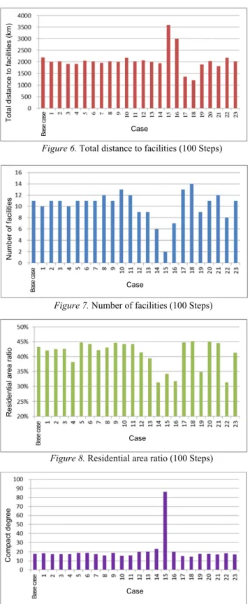
Figures 6, 7, 8 and 9 show the results for each scenario. These results indicate that the element with the greatest influence on the total distance is accessibility, such as the parameter of the distance decay function. When facility accessibility is low, household agents tended to choose the nearest facility and the total distance was shortened. Focusing on Case 15, which has the lowest number of facilities, household agents could use every facility because facility accessibility was high. However, the total distance to facilities in this case was the greatest of all of the cases.
Figure 6. Total distance to facilities (100 Steps)
Figure 7. Number of facilities (100 Steps)
Figure 8. Residential area ratio (100 Steps)
Figure 9. Compact degree (100 Steps)
Case
Base case
Total distance to facilities (km)
Case
Base case
Number of facilities
Case
Base case
Residential area ratio
Case
Base case
Compact degree
Case 14 shows a market mechanism in which highly attractive facilities have remained. It seems that when there is no support from the local government or non-profitable organizations (NPO), facilities will consolidate naturally. Focusing on Cases 14, 15 and 19, the consolidation of residential areas occurred earlier than it did in other cases. These results indicate that the agglutination of residential areas is heavily dependent on the number of facilities. Therefore, the number of facilities suited for a given population and the early agglutination of facilities are the two most influential elements in the creation of a compact urban structure. Focusing on Figure 9, which shows the degree of compactness, Cases 10 and 18 have low values. These results show that the ease of facility maintenance depends on the number of residential areas and facilities.
From the results mentioned above, the key elements influencing the agglutination of residential areas and facilities are the distance decay function and the minimum number of users needed for a facility to sustain service. The minimum number of users indicates the ’strength of the degree of support for service facilities provided by policies’. The fact that facilities with few users naturally consolidated in accordance with market mechanisms in the absence of any support promotes the agglutination of facilities. However, it is hard to say that a lack of support from administrations or NPOs leads to the creation of a compact urban structure because the number of facilities decreases and the quality of social services are low. In addition, the distance decay function means the ’accessibility that attracts household agents to use a facility’. As the parameter becomes smaller, the attractiveness of facilities becomes a key factor in the household agents’ facility choice. Therefore, small (low attractiveness) facilities naturally agglutinate. However, residential areas are widely dispersed throughout the whole area, and the distance to the facility increases. In contrast, when the accessibility of facilities decreases, facility maintenance is easier. Because of this, the possibility of creating a compact urban structure increases.
4. POLICY SIMULATION 4.1 Setting of the Policy Scenarios
Based on the results of the sensitivity analysis, the developed model was adjusted to simulate a more realistic urban and regional spatial structure.
Specifically, this model was set up as follows: 1) in the central area, there is
a high population density with a high aging rate; 2) in areas where the
distance to the central area is greater (suburbs), the population density and
the ratio of young people decreases; and 3) in areas closer to the edge of
virtual space, the aging rate is higher. These are the initial settings for
population placement in this model. Using the adjusted model, two
simulations were conducted according to the assumed policy scenarios
regarding residents and social service facilities. The two assumed scenarios
are as follows: 1) the case in which a mean of transportation leading to high
accessibility is developed through innovation (changing a parameter of the
distance decay function); and 2) the case in which policies aimed at the
maintenance of facilities with the support of the local government or NPOs
are implemented (changing the minimum number of users necessary for the
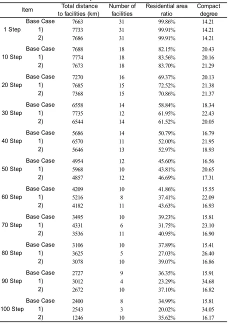
facility to sustain service). The results of these policy simulations are shown in Table 3 and Figure 10.
4.2 Analysis of the Policy Simulation Result
(1) The case in which a parameter of the distance decay function is changed When comparing each index value in Table 3, focusing on 30 steps, there are fewer facilities and a higher compactness compared to the base case. In contrast, the total distance to facilities is greater than in the base case in each step. In addition, the distribution of residential areas in Figure 10 shows that the population density of the central area is high and residential areas are agglutinated in the central area.
In Japan, which is facing long-term population decline, the future development of innovations that allow elderly residents to move easily and safely would result in the residents’ ability to use any facility freely.
Therefore, residents would use the most attractive facility in the central area.
Other facilities would also be agglutinated in the central area. Although a compact urban structure would be created, leaving only a few facilities.
From the perspective of offering social services, it seems that this case is not
Total distance to facilities (km)
Number of facilities
Residential area ratio
Compact degree
Base Case 7663 31 99.86% 14.21
1) 7733 31 99.91% 14.21
2) 7686 31 99.91% 14.21
Base Case 7688 18 82.15% 20.43
1) 7774 18 83.56% 20.16
2) 7673 18 83.70% 21.29
Base Case 7270 16 69.37% 20.13
1) 7685 15 72.52% 21.38
2) 7368 15 70.86% 21.37
Base Case 6558 14 58.84% 18.34
1) 7735 12 61.95% 22.43
2) 6544 14 61.52% 20.05
Base Case 5686 14 50.79% 16.79
1) 6570 11 52.00% 21.95
2) 5646 13 52.97% 18.93
Base Case 4954 12 45.60% 16.56
1) 5968 10 43.81% 20.65
2) 4857 12 46.69% 17.31
Base Case 4209 10 41.86% 15.55
1) 5216 8 37.41% 22.09
2) 4182 11 43.63% 16.93
Base Case 3495 10 39.23% 15.81
1) 4331 6 31.75% 23.10
2) 3536 11 40.95% 16.90
Base Case 3106 10 37.89% 15.41
1) 3625 5 27.03% 26.40
2) 3078 10 39.07% 16.86
Base Case 2727 9 36.35% 15.91
1) 3012 4 23.29% 34.68
2) 2672 10 37.10% 16.82
Base Case 2400 8 34.99% 15.81
1) 2543 3 20.02% 34.05
2) 1246 10 35.62% 16.17
100 Step Item
1 Step
10 Step
20 Step
30 Step
40 Step
50 Step
60 Step
70 Step
80 Step
90 Step
Table 3. Index value of each step
realistic. From the perspective of conserving natural environments in suburban areas, it also seems that this case is not realistic.
(2) The case in which the minimum number of users is changed
When comparing each of the index values in Table 3, the total distance to facilities and the residential area ratio are almost the same as in the base case. After 20 steps, almost every facility has been retained in stark contrast to the results of Scenario 1. In addition, Figure 10 shows the distribution of both the residential areas as well as the facilities that have been retained and that residential areas are dispersed throughout the entire virtual space when the minimum number of users is changed.
From these results, the following findings are indicated when some support is in place, such as grant money from the administration or NPOs.
Some low-revenue facilities will be able to remain and neighborhood- oriented facilities tend to not consolidate in the central area. Instead, they are dispersed throughout the entire virtual space. Similar to the dispersion of facilities, agglutinated residential areas are also dispersed throughout the entire virtual space. Although the number of facilities after 100 steps is greater than in the base case, the degree of compaction is almost the same. In other words, a compact urban structure is formed while retaining the number of facilities that can moderately provide social services to residents. Thus, the following two policy scenarios are deemed important: 1) the promotion
Figure 10. Distribution of residential areas
1 Step 60 Steps 100 Steps
Base case Scenario 1Scenario 2
Legend