Dynamic Linear Hybrid Automata and Their
Applications to Formal Verification of Dynamic Reconfigurable Embedded Systems
著者 柳瀬 龍
著者別表示 Yanase Ryo journal or
publication title
博士論文本文Full 学位授与番号 13301甲第4547号
学位名 博士(工学)
学位授与年月日 2017‑03‑22
URL http://hdl.handle.net/2297/00050238
Dynamic Linear Hybrid Automata and Their Application to Formal Verification of Dynamic
Reconfigurable Embedded Systems
: 1323112012 :
:
DYNAMIC LINEAR HYBRID AUTOMATA AND THEIR APPLICATIONS TO FORMAL VERIFICATION OF DYNAMIC RECONFIGURABLE
EMBEDDED SYSTEMS
Graduate School of Natural Science and Technology, Kanazawa University
by Ryo Yanase February 2016
Dynamic Linear Hybrid Automata and Their Applications to Formal Verification of Dynamic Reconfigurable Embedded Systems
Ryo Yanase Kanazawa University
ABSTRACT
A dynamically reconfigurable system can change its configuration during operation, and stud- ies of such systems are being carried out in many fields. In particular, medical technology and aerospace engineering must ensure system safety because any defect will have serious conse- quences. Model checking is a method for verifying system safety. In this paper, we propose the Dynamic Linear Hybrid Automaton (DLHA) specification language and show a method to analyze reachability for a system consisting of several DLHAs.
Contents
1 Introduction 1
1.1 Background . . . . 1
1.2 Features of dynamically reconfigurable systems consisting of CPUs and DRPs . 1 1.3 Our Proposal . . . . 1
1.3.1 Specification . . . . 1
1.3.2 Verification Method . . . . 2
1.3.3 Experiments on Verifying Dynamically Reconfigurable Systems . . . . . 2
1.4 Related Work . . . . 2
2 Dynamic Linear Hybrid Automaton 3 2.1 Preliminaries . . . . 3
2.2 Syntax . . . . 3
2.3 Operational Semantics . . . . 4
3 Dynamically Reconfigurable Systems 5 3.1 Syntax of DRS . . . . 5
3.2 Semantics of DRS . . . . 6
4 Reachability Analysis 8 4.1 Reachability Problem . . . . 8
4.2 Reachability Analysis . . . . 8
4.2.1 Convex Polyhedra . . . . 8
4.2.2 Algorithm of Reachability Analysis . . . . 9
5 Practical Experiment 14 5.1 Model Checker . . . . 14
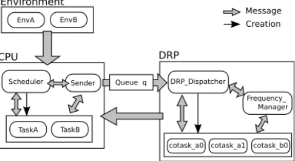
5.2 Specification of Dynamically Reconfigurable Embedded System . . . . 17
5.2.1 A cooperative system including CPU and DRP . . . . 17
5.2.2 Other cases . . . . 20
5.3 Verification Experiment . . . . 21
5.3.1 Schedulability . . . . 23
5.3.2 Creation of co-tasks . . . . 24
5.3.3 Destruction of co-tasks . . . . 24
5.3.4 Frequency management . . . . 25
5.3.5 Tile Management . . . . 25
6 Conclusion and future work 26
A Source Code of the Model Checker 31
1 Introduction
1.1 Background
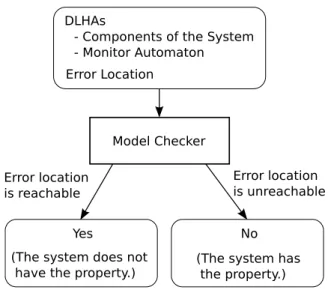
Dynamically reconfigurable systems can change their configuration during operation. Such systems are being used in a number of areas [1, 2, 3] of an apparatus that involves human lives or expensive manufactured goods (e.g., in medical or aerospace engineering). Here, it is very important to guarantee safety. The major methods of checking system safety include simulation and testing; however, it is difficult for them to ensure safety precisely, since large systems can have infinite state spaces. In such a case, model checking that performs exhaustive searches is a more effective method.
In this paper, we propose the Dynamic Linear Hybrid Automaton (DLHA) specification language for describing dynamically reconfigurable systems and provide a reachability analysis algorithm for verifying system safety.
1.2 Features of dynamically reconfigurable systems consisting of CPUs and DRPs
The target of our research is an embedded system in which a CPU and dynamically recon- figurable hardware, e.g., DRP or D-FPGA [4] operate cooperatively. The dynamically recon- figurable processor (DRP) is a coarse-grained programmable processor developed by NEC [3], and it manages both the power conservation and miniaturization. The DRP is used to accel- erate the computations of a general purpose CPU through cooperative operations, and it has the following features:
• Dynamic creation/destruction of functions: when a process occurs, the DRP constitutes a private circuit for processing it. The circuit configuration is released after the process finishes.
• Hybrid property: the operation frequency changes whenever a context switch occurs.
• Parallel execution: the DRP executes several processes on the same board at the same time.
• Queue for communication: the DRP asynchronously receives processing requests from the CPU.
1.3 Our Proposal 1.3.1 Specification
We devised the following new specification techniques for dynamically reconfigurable systems consisting of CPUs and DRPs:
• We use linear hybrid automata [5] describing changes in the operating frequency.
• We use linear hybrid automata that have creation/destruction events describing dynamic creations and destructions of configuration components.
• We use FIFO queues describing asynchronous communication.
We developed a new specification language (DLHA) based on a linear hybrid automaton with both creation/destruction events and unbounded FIFO queues. DLHA is different from existing research in the following points:
• V. Varshavsky and J. Esparza proposed the GALA (Globally Asynchronous - Locally Arbitrary) modeling approach including timed guards [6]. This approach cannot describe hybrid systems since it is the specification language based on discrete systems. Thus, GALA cannot represent changes in operating frequency.
• S. Minami and others have specified a dynamically reconfigurable system using linear hybrid automata and have verified it by using a model checker, HYTECH[7]. Since linear hybrid automata cannot describe changes to the configuration and asynchronous commu- nications, the system has been specified as a static system. Therefore, the specification presented in their work is unsuitable for representing dynamically reconfigurable systems.
Moreover, they verified only the schedulability property of the system, whereas we have verified several other properties in our work.
1.3.2 Verification Method
The originality of our work on the verification method is twofold:
• Our method targets systems that dynamically change their configurations, which is some- thing the existing work, such as HYTECH, has studied. We extend the syntax and seman- tics of linear hybrid automata with special actions calledcreation actionsanddestruction actions. We define a state in which an automaton does not exist and transitions for cre- ation and destruction.
• Our method is a comprehensive symbolic verification for hybrid properties, FIFO queues and creation/destruction of tasks.
1.3.3 Experiments on Verifying Dynamically Reconfigurable Systems
For the experiments, we specified a dynamically reconfigurable embedded system consisting of a CPU and DRP, and verified some of its important features. This is the first time that specification and verification of dynamic changes have been tried in a practical case.
1.4 Related Work
Here, we describe related work and how it differs from our work.
• P. C. Attie and N. A. Lynch specified systems whose components are dynamically cre- ated/destroyed by using I/O automata [8]. I/O automata cannot describe changes in variables, for example, changes in the clock and operating frequency.
• H. Yamada and others proposed hierarchical linear hybrid automata for specifying dy- namically reconfigurable systems [9]. They introduced concepts such as class, object, etc., to the specification language. However, as the scale of the system to be specified increases, the representation and method of analysis in the verification stage tend to be complex.
• B. Boigelot and P. Godefroid specified a communication protocol in terms of finite-state machines and unbounded FIFO buffers (queues), and they verified it [10]. Since the finite-state machine also cannot describe changes in variables, it is unsuitable in our case.
• A. Bouajjani and others proposed a reachability analysis for pushdown automata and a symbolic reachability analysis for FIFO-channel systems [11, 12]. However, since their analysis don’t provide for continuous changes in variables, in languages cannot be used for designing hybrid systems.
2 Dynamic Linear Hybrid Automaton
2.1 Preliminaries
Definition 1 (Constraint). Let V be a finite set of variables. A constraint φ onV is defined as
φ::=true|x∼e|x−y∼e|φ1∧φ2,
wherex, y∈V,e∈Q,φ1andφ2 are constraints onV, and∼∈{=, <, >,≤,≥}. Φ(V)denotes the set of all constraints onV.
Definition 2(Flow condition). Let V ={x1, . . . , xn}be a finite set of (real-valued) variables.
A flow conditionf onV is defined as
f ::= ˙x1 =d1∧. . .∧x˙n =d1, whered1, . . . , dn ∈Q. F(V)is the set of all flow conditions.
For each variable x, we use the dotted variablex, to denote the first derivative of˙ x.
Definition 3 (Update Expression). Let V be a finite set of variables. An update expression upd on V is defined as
upd::=x:=c|x:=x+c,
wherex∈V andc∈Q. UPD(V) is the set of all update expressions can be written.
2.2 Syntax
A dynamic linear hybrid automaton (DLHA) is a tuple (L, V,Inv,Flow,Act, T, t0, Td), where
• Lis a finite set of locations.
• V is a finite set of (real-valued) variables.
• Inv:L→Φ(V) is a function that assigns a constraint to each location.
• Flow:L→F(V) is a function that assigns a flow condition to each location.
• Act=Actin∪Actout∪Actτ is a finite set ofactions.
– Actin is a finite set of input actions, and each input action has the form a?. An input actionm? denotes receiving the message m.
– Actout is a finite set ofoutput actions, and each output action has the forma!. An output actionm! denotes sending the messagemto each DLHA.
– Actτ is a finite set ofinternal actionsthat denote changing a state of a DLHA.
Moreover, we formalize the following special actions:
– Acreation actionthat has the formCrtA′? orCrt A′! denotes a message for creation of DLHAA′. Crt A′?∈Actinis an input action, and it represents thatA′ has been created. Crt A′!∈Actout is an output action, and represents a request for creating A′.
– Adestruction actionthat has the form Dst A′? or CrtA′! denotes a message for a destruction of DLHAA′. Dst A′? ∈Actin is an input action that indicatesA′ has been destroyed.
– An enqueue actionthat has the formq!m denotes enqueueing of messageminto a queueq. This action is an internal one, that is,q!m∈Actτ.
– Adequeue actionthat has the formq?mdenotes dequeueing of messagemfrom the top ofq.
• T ⊆L×Φ(V)×Act×2UPD(V)×Lis a finite set oftransitions. A constraint φ∈Φ(V) is called aguard condition.
• t0∈L×(Actin∪Actτ)×2UPD(V) is aninitial transition.
• Td ⊆L×Φ(V)×Actout is a finite set ofdestruction-transitions.
2.3 Operational Semantics
A stateσ of a DLHA (L, V,Inv,Flow, T, t0, Td) is defined as σ::=⊥|(l,ν),
where l ∈ L is a location, ν : V → R is an assignment called evaluation of variables, and ⊥ denotes anundefined value.
We define the semantics Mof the DLHA by (Σ,⇒,σ0) where
• Σ is a set of states.
• ⇒is a set oftime transitions anddiscrete transitions.
• σ0 is the initial state.
The following rules define time and discrete transitions:
Definition 4 (Time transition of a DLHA). For any δ∈R≥0,
• ⊥⇒δ⊥
• (l,ν)⇒δ (l,ν′) ifν′=ν+δ·Flow(l)∈Inv(l)
where ν′ =ν+δ·Flow(l) denotes an evaluation such that ∀x∈V.ν′(x) =ν(x) +δ·x˙ ∧ Flow(l), and ν′∈Inv(l) denotes thatν′(x) satisfies the constraint Inv(l) for anyx∈V. Definition 5 (Discrete transition of a DLHA). For an evaluation ν and update expressions λ∈2UPD(V),ν[λ] denotes an evaluation updated by λ, that is, for any x∈V,
ν[λ](x) =
⎧⎪
⎨
⎪⎩
c (x:=c∈λ)
ν(x) +c (x:=c̸∈λ, x:=x+c∈λ) ν(x) (otherwise)
• For any transition (l,φ, a,λ, l′)∈T,(l,ν)⇒a(l,ν[λ]) ifν∈φ and ν[λ]∈Inv(l′).
• (Creation of a DLHA) For the initial transition t0 = (l0, a0,λ0),⊥⇒a0 (l0,⃗0[λ0]), where
⃗0 is an evaluation such that∀x∈V.⃗0(x) = 0.
• (Destruction of a DLHA) For any destruction-transition (l,φ, a) ∈ Td, (l,ν) ⇒a⊥ if ν∈φ
For the initial transition (l0, a0,λ0), the initial state σ0 is defined as
σ0=
%⊥ (a0∈Actin) (l0,⃗0[λ0]) (otherwise).
3 Dynamically Reconfigurable Systems
To describe an asynchronous communication among DLHAs in a dynamically reconfigurable system (DRS), we use a queue (unbounded FIFO buffer) as a model of the communication channel. We assume that the system performs lossless transmission, so we can let the queue be unbounded.
3.1 Syntax of DRS
A dynamically reconfigurable system (DRS)S is defined by a tuple (A,Q) consisting of a finite setA={A1, . . . ,A|A|}of DLHAs and a finite setQ={q1, . . . , q|Q|}of queues.
3.2 Semantics of DRS
A states of a DRSS = (A,Q) is a tuple⟨⃗σ,w⃗Q⟩, where
• ⃗σ∈Σ1×· · ·×Σ|A| is a vector of the states of DLHAs.
• w⃗Q∈M1∗×· · ·×M|Q|∗ is a vector of the content of the queues, where eachMi is the set of all messages that can be stored in queueqi.
Definition 6 (Time Transition of a DRS). For an arbitrary δ ∈ R≥0, the time transition is defined as
⟨⃗σ,w⃗Q⟩ →δ ⟨⃗σ′,w⃗Q⟩ ⇐⇒ ∀i.σi⇒δ σi.
Definition 7 (Discrete Transition of a DRS). Let ⃗σ,⃗σ′,w⃗Q and w⃗′Q be ⃗σ = (σ1, . . . ,σ|A|),
⃗σ′ = (σ1′, . . . ,σ|′A|),w⃗Q= (w1, . . . , w|Q|), and w⃗′Q= (w′1, . . . , w′|Q|).
• For any output action a!,⟨⃗σ,w⃗Q⟩ →a⟨⃗σ′,w⃗Q⟩
if∃i.σi⇒a!σi′∧(∀j ̸=i.σj ⇒a?σj
∨((¬∃σj′.σj⇒a?σj′)∧σj =σj′)).
An output action is broadcasted to all DLHAs, and a DLHA receiving the action moves by synchronization if the guard condition holds in the state.
• For an internal action aτ,
– in the case ofaτ =qk!w, ⟨⃗σ,w⃗Q⟩ →qk!w⟨⃗σ′,w⃗′Q⟩,
if(∃i.σi⇒qk!wσi′∧ ∀j ̸=i.σj =σj′)∧wk′ =wkw∧ ∀l̸=k.wk =w′k, – while in the case ofaτ =qk?w, ⟨⃗σ,w⃗Q⟩ →qk?w⟨⃗σ′,w⃗Q′ ⟩,
if (∃i.σi ⇒qk?wσi′∧ ∀j ̸=i.σj =σj′)∧wk =ww′k∧ ∀l̸=k.wl=w′l, – otherwise,⟨⃗σ,w⃗Q⟩ →aτ ⟨⃗σ′,w⃗Q⟩ if∃i.σi⇒aτ σi′∧ ∀j ̸=i.σj =σj′.
Arun (or path)ρ of the systemS is the following finite (or infinite) sequence of states.
ρ:s0→δa00 s1 →δa11 · · ·→δai−1i−1 si→δaii· · · where→δaii betweensi andsi+1is defined as
si→δaii si+1 ⇐⇒ ∃s′i.si →δis′i∧s′i →aisi+1.
The initial states0of a dynamically reconfigurable system is⟨(σ01. . . ,σ0|A|),(w01, . . . , w0|Q|)⟩ where each σ0i is the initial state of DLHAAi and eachw0j is empty; that is,∀j.w0j =ε.
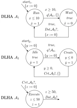
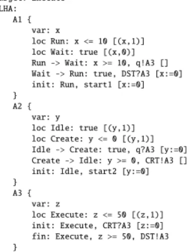
Example 1 (DLHA and DRS). A DLHA is represented by a directed graph, where each node represents a location and each edge represents a transition. Figure 1 shows a dynamically reconfigurable systemS consisting of three DLHAs and one queue.
A1= (L1, V1,Inv1,Flow1,Act1, T1, t01, Td1), A2= (L2, V2,Inv2,Flow2,Act2, T2, t02, Td2), A3= (L3, V3,Inv3,Flow3,Act3, T3, t03, Td3),
S = ({A1,A2,A3},{q}) where
L1={Run,Wait} V1={x}
Inv1={Run4→x≤10,Wait4→true} Flow1={Run4→x˙ = 1,Wait4→x˙ = 0}
Act1={Dst A3?,start1, q!A3}
T1={(Run, x≥10, q!A3,{},Wait), (Wait,true,Dst A3?,{x:= 0},Run)} t01= (Run,start1,{x:= 0})
Td1={}
L2={Idle,Create}
V2={y}
Inv2={Idle4→true,Create4→y≤0} Flow2={Idle4→y˙= 1,Create4→y˙ = 1}
Act2={Crt A3!,start2, q?A3}
T2={(Idle,true, q?A3,{y:= 0},Create), (Create, y≥0,Crt A3!,{},Idle)} t02= (Idle,start2,{y:= 0})
Td2={}
L3={Execute}
V3={z}
Inv3={Execute4→z≤50} Flow3={Execute4→z˙= 1}
Act3={Crt A3?,Dst A3!} T3={}
t03= (Execute,Crt A3?,{z := 0}) Td3={(Execute, z≥50,Dst A3!)} This system runs as follows:
1. A1 requires A3 to be created from A2 by enqueueing a message, and it waits for the message to return from A3.
2. When A2 receives the message, it creates A3.
3. After A3 finishes processing the job, it sends the message to A1 and is destroyed.
4. This system infinitely repeats steps 1) to 3).
For example, (1) shows a run ρof this system is shown.
ρ:⟨((Run, x= 0),(Idle, y= 0),⊥),(ε)⟩
→10q!A3 ⟨((Wait, x= 10),(Idle, y= 0),⊥),(A3)⟩
→0q?A3 ⟨((Wait, x= 10),(Create, y= 0),⊥),(ε)⟩
→0CrtA3 ⟨((Wait, x= 10),(Idle, y= 0), (Execute, z= 0)),(ε)⟩
→50DstA3 ⟨((Run, x= 0),(Idle, y= 0),⊥),(ε)⟩
→· · · (1)
4 Reachability Analysis
4.1 Reachability Problem
We define reachability and the reachability problem for a DRS as follows:
Definition 8 (Reachability). For a DRS S = (A,Q) and a location lt, S reaches lt if there exists a path such that
s0 →δa00 · · ·→δat−1t−1 st
∧st=⟨(σ1, . . . ,σ|A|),w⃗Q⟩,∃k.loc(σk) =lt, where
loc(σ) =
%l (σ= (l,ν))
⊥(undefined) (σ=⊥)
Definition 9 (Reachability Problem). Given a DRSS = (A,Q) and a location lt, we output
“yes” ifS can reach lt, and “no” otherwise.
4.2 Reachability Analysis 4.2.1 Convex Polyhedra
Our method introducesconvex polyhedrafor the reachability analysis in accordance with [17].
A polyhedron is convex if it can be defined by a formula which is a conjunction of linear formulae. For a set V = {x1, . . . , xn} of variables, a convex polyhedron ζ on V is a n- dimensional real space. In particular, we definetrueand false astrue=Rn and false=∅.
DLHA
DLHA
DLHA
Figure 1: Example of DRS consisting of three DLHAs and one queue
Example 2 (Convex Polyhedron). The formula ∃x1. x1≥5∧x2≤1∧x1−x2= 1∧true is a convex polyhedron. From linear formula, the existential quantifier can be eliminated effectively.
Therefore, we obtain
∃x1. x1≥5∧x2≤1∧x1−x2= 1∧true
=∃x1. x1≥5∧x2≤1∧x1−x2= 1
=x2≤1∧x2≥4
=false.
4.2.2 Algorithm of Reachability Analysis
We define a statesin the reachability analysis as (L,ζ,w⃗Q), where
• Lis a finite set of locations.
• ζ is a convex polyhedron.
• w⃗Q is a vector of the content of the queues.
Figure 2, Figure 3 and Figure 4 show the algorithm of the reachability analysis.
Figure 2 is an overview of the reachability analysis, and this algorithm is performed using the expanded method of [13] with a setQof queues. The analysis is performed as follows:
1. Compute an initial state s0 of the systemS (ll.1–3).
2. Initialize a traversed set Visit and a untraversed set Wait of states by∅ and {s0} (line 4).
3. While Wait is not empty, repeat the following process (ll.5–16).
(a) Take a state (L,ζ,w⃗Q) from Wait and remove the state from Wait (ll.6–7).
(b) If the set L of locations contains the target location, return “yes” and terminate (ll.8–10).
(c) If the state has not been traversed yet ((L,ζ,w⃗Q)̸∈Visit) (line 11), i. add the state into Visit (line 12),
ii. compute the setSpost of successors by using the subroutine Succ (line 13), and iii. add all components ofSpost to Wait (line 14).
Subroutine Succ Figure 3 shows the subroutine Succ to compute the successors of a state.
In this algorithm, we make the following assumptions.
S = (A,Q) = ({A1, . . . ,A|A|},{q1, . . . , q|Q|}), Invs=
|A|
&
k=1
Invk, where
Ai= (Li, Vi,Invi,Flowi,Acti, Ti, t0i, Tdi) is a DLHA, t0i= (l0i, a0i,λ0i).
Let the initial state ofS be⟨(σ01, . . . ,σ0|A|)w⃗Q0⟩; s0 is (L0,ζ0,w⃗Q0), where zone (σ) =
%ν (σ= (l,ν)) true (σ=⊥),
L0={loc (σ0i)|σ0i̸=⊥, i∈{1, . . . ,|A|}}, ζ0=
|A|
'
i=0
zone (σ0i).
Here, zone(σ) is a function that assigns a convex polyhedron to each state.
Tsucc(L,ζ) is a function that returns a convex polyhedron after performing a time transi- tion on a given setLof locations and a convex polyhedron ζ (line 4). We define this function in accordance with [17] as follows:
Let the set of all variables in the system and their derivatives beVs=(|A|
k=1Vk ={x1, . . . , xn} and ˙Vs={x˙1, . . . ,x˙n}.
Tsucc(L,ζ) =∃x1, . . . , xn∈Vs.∃δ∈R≥0.∃x˙1, . . . ,x˙n ∈V˙s. ζ∧Flow(L)∧ '
x∈Vs
x′=x+δx˙ and rename x′ asx,
where
Flows=
|A|
&
k=1
Flowk, Flow= '
l∈L
Flows(l).
For a convex polyhedron ζ and a set λ of update expressions, ζ[λ] denotes the convex polyhedron updated byλ for ζ. Let the set of reset variables and set of shifted variables be Vr = {x| x:=c∈λ}={xr1, . . . , xrm} and Va ={x|x:=x+c∈λ}={xa1, . . . , xan}. ζ[λ]
can be computed as
ζ[λ] = (∃xr1, . . . , xrm∈Vr.ζa)∧ '
x∈Vr
x=mr(x),
where
mr ={x4→c|x:=c∈λ}, ma={x4→c|x:=x+c∈λ},
ζa=∃xa1, . . . , xan∈Va. ζ∧ '
x∈Va
x′ =x+ma(x) and rename variablesx′ asx.
Given a state (L,ζ,w⃗Q) and a system, the successors are computed using the procedure described below.
1. For each transition (l,φ, a,λ, l′) (or destruction-transition (l,φ, al!)) outgoing from a lo- cationl∈L, the setSpost of post states is computed as follows (ll.5–31):
(a) Compute the convex polyhedron for the time transition (line 4).
ζδ = Tsucc(L,ζ)∧ '
lp∈L
Invs(lp).
(b) Ifa is an internal action,Spost is computed as follows:
i. Compute the set of locations (line 8)
L′= (L\ {l})∪{l′}.
ii. Compute the convex polyhedron for the discrete transition (line 9) ζ′ = (ζ∧φ)[λ]∧ '
l′p∈L′
Invs(l′p).
iii. Ifais an enqueue actionqk!w (ll.11–15), Spost=
%{(L′,ζ′,w⃗′Q)} (ζ′ ̸=false)
∅ (otherwise),
where
⃗
w′Q= (w1, . . . , wk−1, wk·w, wk+1, . . . , w|Q|).
iv. If ais a dequeue action qk?w(ll.16–20),
Spost=
⎧⎪
⎨
⎪⎩
{(L′,ζ′,w⃗′Q)} (ζ′̸=false, wk=w·wk′,
∀j ̸=k.wj =wj′)
∅ (otherwise).
v. If ais another internal action (line 22), Spost=
%{(L′,ζ′,w⃗Q)} (ζ′̸=false)
∅ (otherwise).
(c) If a is an output action al!, Spost is computed with the subroutine Syncs (line 26 and 29).
(d) Ifa is an input action,Spost=∅.
Subroutine Syncs Figure 4 shows the subroutine Syncs of Succ to compute successors by using the transition that has an output action. Given a state (L,ζ,w⃗Q), a transition (or destruction-transition)ts= (l,φg, al!,λ, l′), and a system S = (A,Q), a set Spost of successors is computed as follows:
1. InitializeSpost as∅(line 1).
2. Compute a convex polyhedron ζδ for the time transition (line 2).
ζδ = Tsucc(L,ζ)∧ '
lp∈L
Invs(lp).
3. For eachAi in the system S, compute the setTsi of transitions that are outgoing from the state by using an input actional? (ll.3–5),
Tsi={(li,φi, al?,λi, li′)∈Ti|li∈(L\ {l})}.
4. Compute the set ∆of combinations ofTsi (line 6).
∆=)
{Tsi|Tsi ̸=∅, i∈{1, . . . ,|A|}}.
5. For each combination T = (t1, . . . , tn) ∈ ∆, the successor (L′T,ζT′ ,w⃗Q) is computed as follows (ll.7–29):
(a) Compute the setTsync of transitions (line 9).
Tsync= max
|∆′| ∆′ ⊆{t1, . . . , tn} s. t. ζδ∧φ∧'
{φs|(l1,φs, al?,λs, l2)∈∆′}̸=false.
(b) Compute the setL′T of locations (ll.9–14, line 21).
L′T = (L\Lpre)∪Lpost, where
Lsync={l1 |(l1,φs, al?,λs, l2)∈Tsync}, L′sync={l2 |(l2,φs, al?,λs, l2)∈Tsync},
Lpre={l}∪Lsync
Lpost=
⎧⎪
⎨
⎪⎩
{l′, lj0}∪L′sync (al=Crt Aj, L∩Lj=∅) L′sync (al=Dst Aj)
{l′}∪L′sync (otherwise).
(c) Compute the update expressionλsync (ll.9–14).
λsync=
⎧⎪
⎨
⎪⎩
λ∪λ0j∪λin (al=Crt Aj, L∩Lj =∅) λin (al=Dst Aj)
λ∪λin (otherwise), where
λin=&
{λs|(l1,φs, al?,λs, l2)∈Tsync}.
(d) Compute the conjunction of guard conditions (ll.9–14).
φsync=φ∧'
{φs|(l1,φs, al?,λs, l2)∈Tsync}.
(e) Compute the convex polyhedronζT′ (ll.22–24).
ζT′ =
%∃xj1, . . . , xj|Vj| ∈Vj.ζ′ (al=Dst Aj)
ζ′ (otherwise),
where
ζ′ = (ζδ∧φsync)[λsync]∧ '
lp′∈L′
Invs(l′p).