Unpublished document available at
http://www.res.otaru-uc.ac.jp/~emt-hogasa/, https://barrel.repo.nii.ac.jp/.
January, 2019
Supplemental tables and R codes for the paper
“Asymptotic cumulants of the minimum phi-divergence estimator for categorical data under possible model misspecification”
Haruhiko Ogasawara
This article supplements Ogasawara (2019a, b).
Part 1 gives numerical results under correct model specification in Tables S2.1 to S2.13. In the tables, “.00” indicates a rounded value of zero up to the second place while “0”
indicates an exactly zero value.
Part 2 gives R codes and examples of running the programs.
References
Ogasawara, H. (2019a). Asymptotic cumulants of the minimum phi-divergence estimator for categorical data under possible model misspecification. To appear in
Communications in Statistics – Theory and Methods.Ogasawara, H. (2019b). Supplement to the paper “Asymptotic cumulants of the minimum phi-divergence estimator for categorical data under possible model misspecification”.
To appear in
Economic Review (Otaru University of Commerce), 70(2 & 3).
http://www.res.otaru-uc.ac.jp/~emt-hogasa/, https://barrel.repo.nii.ac.jp/.
Part 1. Numerical results under correct model specification
Table S2.1. True probabilities under correct model misspecification
Case τ'
A: The genetics of plants (Fisher, 1970)
.6000 .1500 .1500 .1000
B: 3-category truncated Poisson variate (Bishop et al., 1975)
.3679 .3679 .2642
C: 4-category truncated Poisson variate
.2231 .3347 .2510 .1912
D: 4-category redundant truncated Poisson variate
.2231 .3347 .2510 .1912
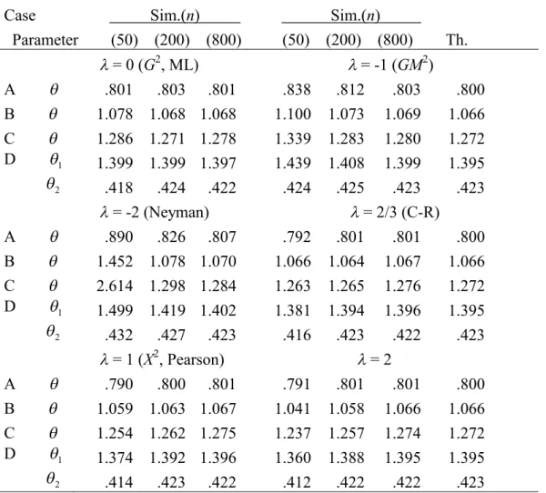
Table S2.2. Simulated and theoretical standard errors multiplied by n1/2 for the MEs when models are true: 21/2
Case Sim.(n) Sim.(n)
Parameter (50) (200) (800) (50) (200) (800) Th.
= 0 (G2, ML) = -1 (GM2)
A .801 .803 .801 .838 .812 .803 .800
B 1.078 1.068 1.068 1.100 1.073 1.069 1.066 C 1.286 1.271 1.278 1.339 1.283 1.280 1.272 D 1 1.399 1.399 1.397 1.439 1.408 1.399 1.395
2 .418 .424 .422 .424 .425 .423 .423
= -2 (Neyman) = 2/3 (C-R)
A .890 .826 .807 .792 .801 .801 .800
B 1.452 1.078 1.070 1.066 1.064 1.067 1.066 C 2.614 1.298 1.284 1.263 1.265 1.276 1.272 D 1 1.499 1.419 1.402 1.381 1.394 1.396 1.395
2 .432 .427 .423 .416 .423 .422 .423
= 1 (X2, Pearson) = 2
A .790 .800 .801 .791 .801 .801 .800
B 1.059 1.063 1.067 1.041 1.058 1.066 1.066 C 1.254 1.262 1.275 1.237 1.257 1.274 1.272 D 1 1.374 1.392 1.396 1.360 1.388 1.395 1.395
2 .414 .423 .422 .412 .422 .422 .423 Note.n= the number of observations, Sim. = simulated value, Th. = theoretical value =21/2,G2= the log-likelihood ratio statistic,GM2= the modified
log-likelihood ratio statistic, Neyman = Neyman’s statistic, C-R = the Cressie-Read statistic,X2= Pearson’s statistic.
Table S2.2. (continued)
n: 50 200 800
Case Z NC Z NC Z NC
A 579 95 0 0 0 0
B 0 10 0 0 0 0
C 3 9 0 0 0 0
D 3 3251 0 2 0 0
Note.n= the number of observations, Z = the number of deleted cases with zero frequenc(ies), NC = the number of deleted cases due to non-convergence.
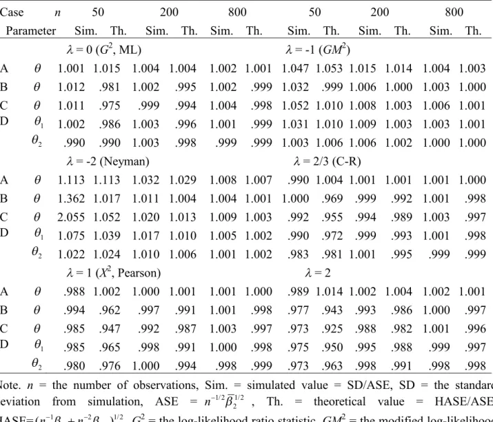
Table S2.3. Simulated and theoretical ratios of the higher- and lower-order asymptotic standard errors for the MEs when models are true
Case n 50 200 800 50 200 800
Parameter Sim. Th. Sim. Th. Sim. Th. Sim. Th. Sim. Th. Sim. Th.
= 0 (G2, ML) = -1 (GM2)
A 1.001 1.015 1.004 1.004 1.002 1.001 1.047 1.053 1.015 1.014 1.004 1.003 B 1.012 .981 1.002 .995 1.002 .999 1.032 .999 1.006 1.000 1.003 1.000 C 1.011 .975 .999 .994 1.004 .998 1.052 1.010 1.008 1.003 1.006 1.001 D 1 1.002 .986 1.003 .996 1.001 .999 1.031 1.010 1.009 1.003 1.003 1.001
2 .990 .990 1.003 .998 .999 .999 1.003 1.006 1.006 1.002 1.000 1.000
= -2 (Neyman) = 2/3 (C-R)
A 1.113 1.113 1.032 1.029 1.008 1.007 .990 1.004 1.001 1.001 1.001 1.000 B 1.362 1.017 1.011 1.004 1.004 1.001 1.000 .969 .999 .992 1.001 .998 C 2.055 1.052 1.020 1.013 1.009 1.003 .992 .955 .994 .989 1.003 .997 D 1 1.075 1.039 1.017 1.010 1.005 1.002 .990 .972 .999 .993 1.001 .998
2 1.022 1.024 1.010 1.006 1.001 1.002 .983 .981 1.001 .995 .999 .999
= 1 (X2, Pearson) = 2
A .988 1.002 1.000 1.001 1.001 1.000 .989 1.014 1.002 1.004 1.002 1.001 B .994 .962 .997 .991 1.001 .998 .977 .943 .993 .986 1.000 .997 C .985 .947 .992 .987 1.003 .997 .973 .925 .988 .982 1.001 .996 D 1 .985 .965 .998 .991 1.000 .998 .975 .950 .995 .988 .999 .997
2 .980 .976 1.000 .994 .998 .999 .973 .963 .998 .991 .998 .998 Note. n = the number of observations, Sim. = simulated value = SD/ASE, SD = the standard deviation from simulation, ASE = n1/221/2 , Th. = theoretical value = HASE/ASE, HASE=(n12n22)1/2,G2 = the log-likelihood ratio statistic,GM2= the modified log-likelihood ratio statistic, Neyman = Neyman’s statistic, C-R = the Cressie-Read statistic, X2 = Pearson’s statistic.
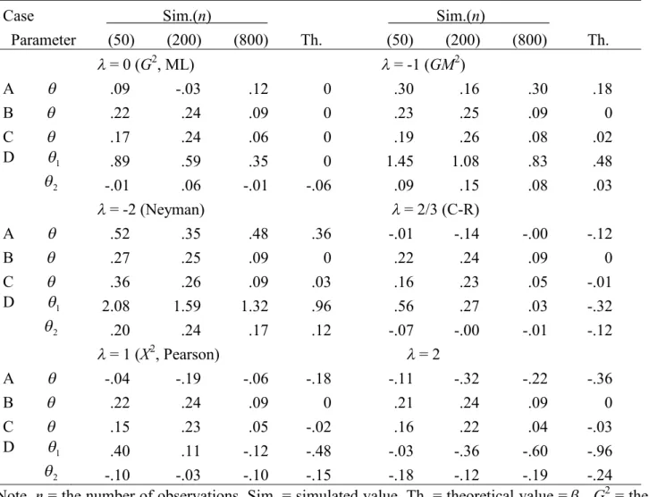
Table S2.4. Simulated and theoretical biases multiplied bynfor the MEs when models are true: 1
Case Sim.(n) Sim.(n)
Parameter (50) (200) (800) Th. (50) (200) (800) Th.
= 0 (G2, ML) = -1 (GM2)
A .09 -.03 .12 0 .30 .16 .30 .18
B .22 .24 .09 0 .23 .25 .09 0
C .17 .24 .06 0 .19 .26 .08 .02
D 1 .89 .59 .35 0 1.45 1.08 .83 .48
2 -.01 .06 -.01 -.06 .09 .15 .08 .03
= -2 (Neyman) = 2/3 (C-R)
A .52 .35 .48 .36 -.01 -.14 -.00 -.12
B .27 .25 .09 0 .22 .24 .09 0
C .36 .26 .09 .03 .16 .23 .05 -.01
D 1 2.08 1.59 1.32 .96 .56 .27 .03 -.32
2 .20 .24 .17 .12 -.07 -.00 -.01 -.12
= 1 (X2, Pearson) = 2
A -.04 -.19 -.06 -.18 -.11 -.32 -.22 -.36
B .22 .24 .09 0 .21 .24 .09 0
C .15 .23 .05 -.02 .16 .22 .04 -.03
D 1 .40 .11 -.12 -.48 -.03 -.36 -.60 -.96
2 -.10 -.03 -.10 -.15 -.18 -.12 -.19 -.24 Note. n= the number of observations, Sim. = simulated value, Th. = theoretical value =1,G2 = the log-likelihood ratio statistic,GM2 = the modified log-likelihood ratio statistic, Neyman = Neyman’s statistic, C-R = the Cressie-Read statistic, X2= Pearson’s statistic. The “0” indicates an exactly zero value.
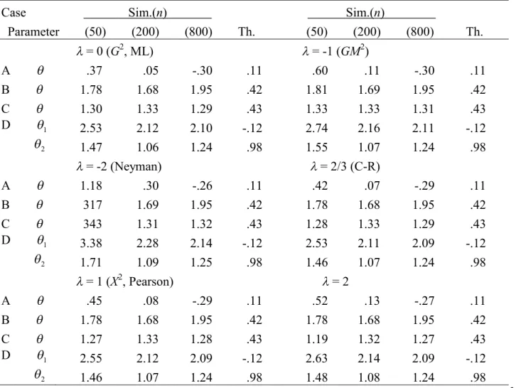
Table S2.5. Simulated and theoretical skewnesses multiplied by n1/2 for the MEs when models are true: 3/ 23/2
Case Sim.(n) Sim.(n)
Parameter (50) (200) (800) Th. (50) (200) (800) Th.
= 0 (G2, ML) = -1 (GM2)
A .37 .05 -.30 .11 .60 .11 -.30 .11
B 1.78 1.68 1.95 .42 1.81 1.69 1.95 .42
C 1.30 1.33 1.29 .43 1.33 1.33 1.31 .43
D 1 2.53 2.12 2.10 -.12 2.74 2.16 2.11 -.12
2 1.47 1.06 1.24 .98 1.55 1.07 1.24 .98
= -2 (Neyman) = 2/3 (C-R)
A 1.18 .30 -.26 .11 .42 .07 -.29 .11
B 317 1.69 1.95 .42 1.78 1.68 1.95 .42
C 343 1.31 1.32 .43 1.28 1.33 1.29 .43
D 1 3.38 2.28 2.14 -.12 2.53 2.11 2.09 -.12
2 1.71 1.09 1.25 .98 1.46 1.07 1.24 .98
= 1 (X2, Pearson) = 2
A .45 .08 -.29 .11 .52 .13 -.27 .11
B 1.78 1.68 1.95 .42 1.78 1.68 1.95 .42
C 1.27 1.33 1.28 .43 1.19 1.32 1.27 .43
D 1 2.55 2.12 2.09 -.12 2.63 2.14 2.09 -.12
2 1.46 1.07 1.24 .98 1.48 1.08 1.24 .98
Note. n= the number of observations, Sim. = simulated value, Th. = theoretical value = 3/ 23/2,G2
= the log-likelihood ratio statistic, GM2 = the modified log-likelihood ratio statistic, Neyman = Neyman’s statistic, C-R = the Cressie-Read statistic,X2= Pearson’s statistic.
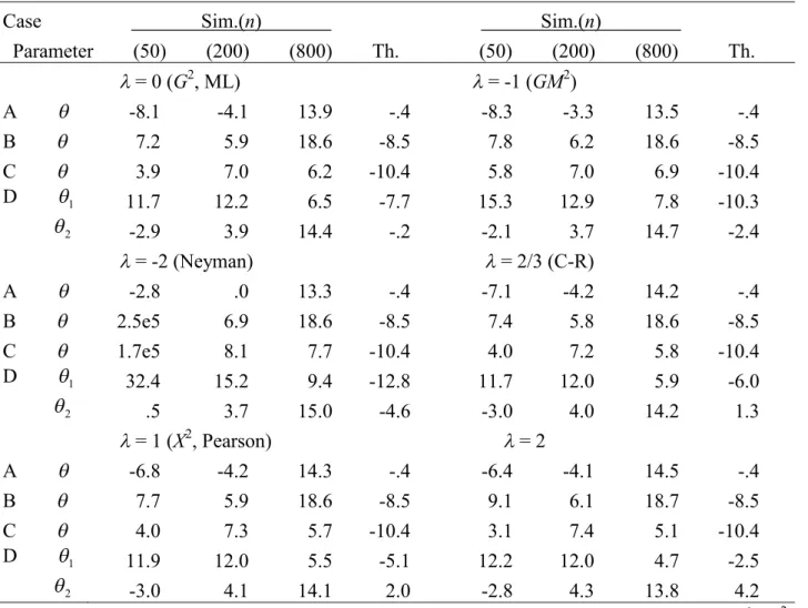
Table S2.6. Simulated and theoretical kurtoses multiplied by n for the MEs when models are true: 4/ 22
Case Sim.(n) Sim.(n)
Parameter (50) (200) (800) Th. (50) (200) (800) Th.
= 0 (G2, ML) = -1 (GM2)
A -8.1 -4.1 13.9 -.4 -8.3 -3.3 13.5 -.4
B 7.2 5.9 18.6 -8.5 7.8 6.2 18.6 -8.5
C 3.9 7.0 6.2 -10.4 5.8 7.0 6.9 -10.4
D 1 11.7 12.2 6.5 -7.7 15.3 12.9 7.8 -10.3
2 -2.9 3.9 14.4 -.2 -2.1 3.7 14.7 -2.4
= -2 (Neyman) = 2/3 (C-R)
A -2.8 .0 13.3 -.4 -7.1 -4.2 14.2 -.4
B 2.5e5 6.9 18.6 -8.5 7.4 5.8 18.6 -8.5
C 1.7e5 8.1 7.7 -10.4 4.0 7.2 5.8 -10.4
D 1 32.4 15.2 9.4 -12.8 11.7 12.0 5.9 -6.0
2 .5 3.7 15.0 -4.6 -3.0 4.0 14.2 1.3
= 1 (X2, Pearson) = 2
A -6.8 -4.2 14.3 -.4 -6.4 -4.1 14.5 -.4
B 7.7 5.9 18.6 -8.5 9.1 6.1 18.7 -8.5
C 4.0 7.3 5.7 -10.4 3.1 7.4 5.1 -10.4
D 1 11.9 12.0 5.5 -5.1 12.2 12.0 4.7 -2.5
2 -3.0 4.1 14.1 2.0 -2.8 4.3 13.8 4.2
Note.n= the number of observations, Sim. = simulated value, Th. = theoretical value = 4 / 22,G2= the log-likelihood ratio statistic, GM2 = the modified log-likelihood ratio statistic, Neyman = Neyman’s statistic, C-R = the Cressie-Read statistic,X2= Pearson’s statistic, ex y x 10y.
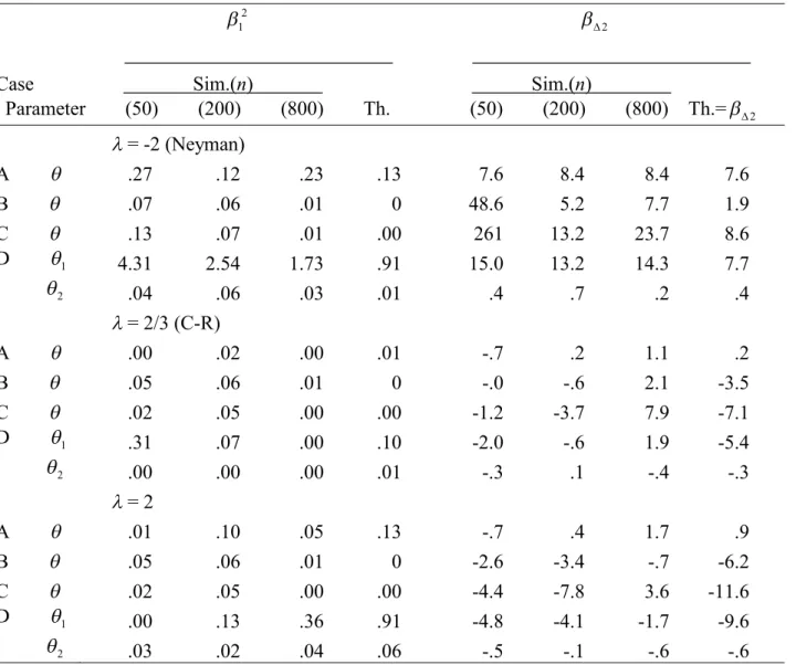
Table S2.7. Simulated and squared biases and added higher-order asymptotic biases multiplied by n2 for the MEs when models are true: 12 and 2
2
1 2
Case Sim.(n) Sim.(n)
Parameter (50) (200) (800) Th. (50) (200) (800) Th.=2
= -2 (Neyman)
A .27 .12 .23 .13 7.6 8.4 8.4 7.6
B .07 .06 .01 0 48.6 5.2 7.7 1.9
C .13 .07 .01 .00 261 13.2 23.7 8.6
D 1 4.31 2.54 1.73 .91 15.0 13.2 14.3 7.7
2 .04 .06 .03 .01 .4 .7 .2 .4
= 2/3 (C-R)
A .00 .02 .00 .01 -.7 .2 1.1 .2
B .05 .06 .01 0 -.0 -.6 2.1 -3.5
C .02 .05 .00 .00 -1.2 -3.7 7.9 -7.1
D 1 .31 .07 .00 .10 -2.0 -.6 1.9 -5.4
2 .00 .00 .00 .01 -.3 .1 -.4 -.3
= 2
A .01 .10 .05 .13 -.7 .4 1.7 .9
B .05 .06 .01 0 -2.6 -3.4 -.7 -6.2
C .02 .05 .00 .00 -4.4 -7.8 3.6 -11.6
D 1 .00 .13 .36 .91 -4.8 -4.1 -1.7 -9.6
2 .03 .02 .04 .06 -.5 -.1 -.6 -.6
Note. n= the number of observations, Sim. = simulated value, Th. = theoretical value =12 or 2, Neyman = Neyman’s statistic, C-R = the Cressie-Read statistic. The “0” indicates an exactly zero value.
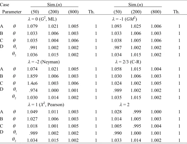
Table S2.8. Simulated and theoretical standard errors of the studentized MEs when models are true: 21/2'
Case Sim.(n) Sim.(n)
Parameter (50) (200) (800) Th. (50) (200) (800) Th.
= 0 (G2, ML) = -1 (GM2)
A 1.079 1.021 1.005 1 1.093 1.025 1.006 1
B 1.033 1.006 1.003 1 1.033 1.006 1.003 1
C 1.035 1.004 1.006 1 1.038 1.005 1.006 1
D 1 .991 1.002 1.002 1 .987 1.002 1.002 1
2 1.036 1.015 1.002 1 1.034 1.015 1.002 1
= -2 (Neyman) = 2/3 (C-R)
A 1.074 1.021 1.005 1 1.058 1.015 1.004 1
B 1.859 1.006 1.003 1 1.030 1.006 1.003 1
C 1.4e6 1.003 1.006 1 1.024 1.002 1.005 1
D 1 .974 1.000 1.001 1 .989 1.002 1.002 1
2 1.030 1.014 1.002 1 1.035 1.015 1.002 1
= 1 (X2, Pearson) = 2
A 1.049 1.011 1.003 1 1.028 .999 1.000 1
B 1.027 1.006 1.003 1 1.014 1.005 1.003 1
C 1.018 1.001 1.005 1 1.005 .995 1.004 1
D 1 .989 1.002 1.002 1 .990 1.000 1.001 1
2 1.034 1.015 1.002 1 1.033 1.014 1.002 1
Note.n= the number of observations, Sim. = simulated value, Th. = theoretical value =21/2'=1,G2= the log-likelihood ratio statistic, GM2 = the modified log-likelihood ratio statistic, Neyman = Neyman’s statistic, C-R = the Cressie-Read statistic,X2= Pearson’s statistic, ex y x 10y.
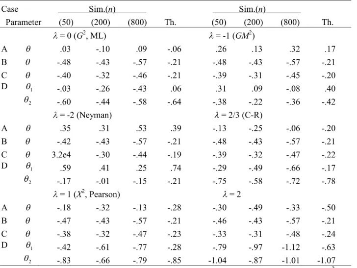
Table S2.9. Simulated and theoretical biases multiplied by n1/2 for the studentized MEs when models are true: 1'
Case Sim.(n) Sim.(n)
Parameter (50) (200) (800) Th. (50) (200) (800) Th.
= 0 (G2, ML) = -1 (GM2)
A .03 -.10 .09 -.06 .26 .13 .32 .17
B -.48 -.43 -.57 -.21 -.48 -.43 -.57 -.21
C -.40 -.32 -.46 -.21 -.39 -.31 -.45 -.20
D 1 -.03 -.26 -.43 .06 .31 .09 -.08 .40
2 -.60 -.44 -.58 -.64 -.38 -.22 -.36 -.42
= -2 (Neyman) = 2/3 (C-R)
A .35 .31 .53 .39 -.13 -.25 -.06 -.20
B -.42 -.43 -.57 -.21 -.48 -.43 -.57 -.21
C 3.2e4 -.30 -.44 -.19 -.39 -.32 -.47 -.22
D 1 .59 .41 .25 .74 -.29 -.49 -.66 -.17
2 -.17 -.01 -.15 -.21 -.75 -.58 -.72 -.78
= 1 (X2, Pearson) = 2
A -.18 -.32 -.13 -.28 -.30 -.49 -.33 -.50
B -.47 -.43 -.57 -.21 -.46 -.43 -.57 -.21
C -.38 -.32 -.47 -.23 -.33 -.31 -.48 -.24
D 1 -.42 -.61 -.77 -.28 -.79 -.97 -1.12 -.63
2 -.83 -.66 -.79 -.85 -1.04 -.87 -1.01 -1.07
Note.n= the number of observations, Sim. = simulated value, Th. = theoretical value =1',G2= the log-likelihood ratio statistic,GM2 = the modified log-likelihood ratio statistic, Neyman = Neyman’s statistic, C-R = the Cressie-Read statistic,X2= Pearson’s statistic, ex y x 10y.
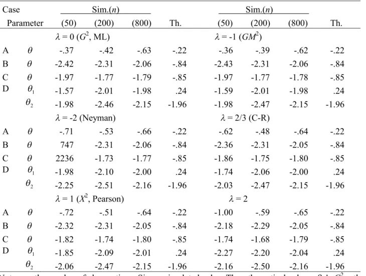
Table S2.10. Simulated and theoretical skewnesses multiplied by n1/2 for the studentized MEs when models are true: 3'
Case Sim.(n) Sim.(n)
Parameter (50) (200) (800) Th. (50) (200) (800) Th.
= 0 (G2, ML) = -1 (GM2)
A -.37 -.42 -.63 -.22 -.36 -.39 -.62 -.22
B -2.42 -2.31 -2.06 -.84 -2.43 -2.31 -2.06 -.84
C -1.97 -1.77 -1.79 -.85 -1.97 -1.77 -1.78 -.85
D 1 -1.57 -2.01 -1.98 .24 -1.59 -2.01 -1.98 .24
2 -1.98 -2.46 -2.15 -1.96 -1.98 -2.47 -2.15 -1.96
= -2 (Neyman) = 2/3 (C-R)
A -.71 -.53 -.66 -.22 -.62 -.48 -.64 -.22
B 747 -2.31 -2.06 -.84 -2.36 -2.31 -2.05 -.84
C 2236 -1.73 -1.77 -.85 -1.86 -1.75 -1.80 -.85
D 1 -1.98 -2.10 -2.00 .24 -1.74 -2.06 -2.00 .24
2 -2.25 -2.51 -2.16 -1.96 -2.03 -2.47 -2.15 -1.96
= 1 (X2, Pearson) = 2
A -.72 -.51 -.64 -.22 -1.00 -.59 -.65 -.22
B -2.32 -2.31 -2.05 -.84 -2.18 -2.29 -2.05 -.84
C -1.82 -1.74 -1.80 -.85 -1.74 -1.68 -1.79 -.85
D 1 -1.85 -2.09 -2.01 .24 -2.27 -2.20 -2.04 .24
2 -2.06 -2.47 -2.15 -1.96 -2.16 -2.50 -2.16 -1.96
Note.n= the number of observations, Sim. = simulated value, Th. = theoretical value =3',G2= the log-likelihood ratio statistic,GM2 = the modified log-likelihood ratio statistic, Neyman = Neyman’s statistic, C-R = the Cressie-Read statistic,X2= Pearson’s statistic.
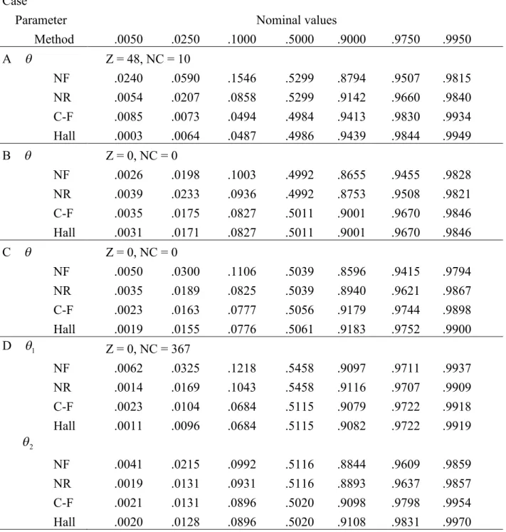
Table S2.11. Proportions of a population value below the one-sided confidence intervals when models are true:n= 50 and 2 (Neyman’s statistic)
Case
Parameter Method
Nominal values
.0050 .0250 .1000 .5000 .9000 .9750 .9950
A
NF NR C-F Hall
Z = 48, NC = 10
.0240 .0590 .1546 .5299 .8794 .9507 .9815 .0054 .0207 .0858 .5299 .9142 .9660 .9840 .0085 .0073 .0494 .4984 .9413 .9830 .9934 .0003 .0064 .0487 .4986 .9439 .9844 .9949
B
NF NR C-F Hall
Z = 0, NC = 0
.0026 .0198 .1003 .4992 .8655 .9455 .9828 .0039 .0233 .0936 .4992 .8753 .9508 .9821 .0035 .0175 .0827 .5011 .9001 .9670 .9846 .0031 .0171 .0827 .5011 .9001 .9670 .9846
C
NF NR C-F Hall
Z = 0, NC = 0
.0050 .0300 .1106 .5039 .8596 .9415 .9794 .0035 .0189 .0825 .5039 .8940 .9621 .9867 .0023 .0163 .0777 .5056 .9179 .9744 .9898 .0019 .0155 .0776 .5061 .9183 .9752 .9900 D 1
NF NR C-F Hall
Z = 0, NC = 367
.0062 .0325 .1218 .5458 .9097 .9711 .9937 .0014 .0169 .1043 .5458 .9116 .9707 .9909 .0023 .0104 .0684 .5115 .9079 .9722 .9918 .0011 .0096 .0684 .5115 .9082 .9722 .9919
2
NF NR C-F Hall
.0041 .0215 .0992 .5116 .8844 .9609 .9859 .0019 .0131 .0931 .5116 .8893 .9637 .9857 .0021 .0131 .0896 .5020 .9098 .9798 .9954 .0020 .0128 .0896 .5020 .9108 .9831 .9970
Note. NF = the normal approximation by the Fisher information matrix, NR = the normal approximation by the robust ASE estimate, C-F = the Cornish-Fisher expansion, Hall = Hall’s (1992) monotonic cubic transformation, Z = the number of deleted cases with zero frequenc(ies), NC = the number of deleted case(s) due to non-convergence.
Table S2.12. Proportions of a population value below the one-sided confidence intervals when models are true:n= 50 and 2 / 3 (the Cressie-Read statistic)
Case
Parameter Method
Nominal values
.0050 .0250 .1000 .5000 .9000 .9750 .9950
A
NF NR C-F Hall
Z = 48, NC = 10
.0105 .0317 .1125 .5048 .8833 .9606 .9873 .0127 .0380 .1096 .5048 .8827 .9553 .9831 .0048 .0274 .1074 .5161 .9053 .9701 .9871 .0042 .0240 .1074 .5161 .9054 .9847 .9893
B
NF NR C-F Hall
Z = 0, NC = 0
.0016 .0147 .0798 .4992 .8872 .9604 .9875 .0016 .0169 .0831 .4992 .8831 .9584 .9852 .0021 .0189 .0841 .4992 .8949 .9628 .9902 .0021 .0189 .0841 .4992 .8949 .9629 .9904
C
NF NR C-F Hall
Z = 0, NC = 0
.0016 .0173 .0879 .5053 .8894 .9642 .9899 .0025 .0192 .0895 .5053 .8863 .9592 .9874 .0034 .0214 .1004 .5058 .8899 .9646 .9899 .0034 .0213 .1004 .5058 .8904 .9653 .9906 D 1
NF NR C-F Hall
Z = 0, NC = 367
.0022 .0156 .0832 .5030 .9000 .9689 .9932 .0026 .0168 .0856 .5030 .8944 .9660 .9930 .0006 .0138 .0855 .5196 .8947 .9710 .9949 .0006 .0122 .0855 .5196 .8947 .9710 .9949
2
NF NR C-F Hall
.0020 .0154 .0766 .4715 .8728 .9554 .9843 .0025 .0162 .0790 .4715 .8746 .9544 .9836 .0038 .0217 .0987 .5001 .9045 .9800 .9955 .0037 .0217 .0987 .5001 .9049 .9833 .9988
Note. NF = the normal approximation by the Fisher information matrix, NR = the normal approximation by the robust ASE estimate, C-F = the Cornish-Fisher expansion, Hall = Hall’s (1992) monotonic cubic transformation, Z = the number of deleted cases with zero frequenc(ies), NC = the number of deleted cases due to non-convergence.
Table S2.13. Proportions of a population value below the one-sided confidence intervals when models are true:n= 50 and 2
Case
Parameter Method
Nominal values
.0050 .0250 .1000 .5000 .9000 .9750 .9950
A
NF NR C-F Hall
Z = 48, NC = 10
.0091 .0347 .1067 .4945 .8771 .9589 .9862 .0132 .0318 .0973 .4945 .8893 .9514 .9827 .0084 .0290 .0906 .5167 .8966 .9566 .9885 .0052 .0238 .0892 .5168 .9004 .9606 .9901
B
NF NR C-F Hall
Z = 0, NC = 0
.0015 .0145 .0778 .4992 .8895 .9619 .9883 .0024 .0191 .0832 .4992 .8823 .9584 .9827 .0041 .0234 .0932 .4992 .8754 .9468 .9730 .0041 .0234 .0932 .4992 .8754 .9472 .9744
C
NF NR C-F Hall
Z = 0, NC = 0
.0010 .0149 .0832 .5041 .8939 .9660 .9908 .0048 .0224 .0871 .5041 .8947 .9601 .9932 .0058 .0272 .1005 .5056 .8903 .9642 .9845 .0051 .0271 .1005 .5065 .8904 .9674 .9859 D 1
NF NR C-F Hall
Z = 0, NC = 367
.0022 .0118 .0699 .4779 .8908 .9643 .9928 .0014 .0133 .0757 .4779 .8900 .9538 .9895 .0013 .0156 .0832 .5164 .8996 .9681 .9899 .0012 .0154 .0832 .5164 .8996 .9681 .9899
2
NF NR C-F Hall
.0018 .0135 .0706 .4510 .8690 .9531 .9829 .0021 .0134 .0675 .4510 .8533 .9564 .9834 .0046 .0236 .0993 .5109 .9132 .9683 .9932 .0046 .0232 .0993 .5109 .9137 .9725 .9947
Note. NF = the normal approximation by the Fisher information matrix, NR = the normal approximation by the robust ASE estimate, C-F = the Cornish-Fisher expansion, Hall = Hall’s (1992) monotonic cubic transformation, Z = the number of deleted cases with zero frequenc(ies), NC = the number of deleted cases due to non-convergence.
Part 2. R codes and examples of running the programs
In Part 2, two examples are shown. In Example 1, log-linear models in a 2 2 2 × × contingency table are analyzed using the program “mpe3a.R”. In Example 2, log-linear models including the linear-by-linear model in a two-way contingency table are dealt with by the program “mpe2a.R”. In these programs the function “mpese” is used.
Example 1.
The program “mpe3a.R”
#
# Robust asymptotic standard errors of the minimizing phi-divergence
# estimators (MPEs) for log-linear models in a 2x2x2 table
# under possible model misspecification
#
# <mpe3a.R> April 16, 2018
#
# Use as: R prompt >source('file_name').
# The results will be given in 'r.u'.
#
starttime=proc.time() sink ('r.u')
print(date(),quote=F)
###### function mpese
mpese=function(n,pr,al,w,qo,iq,ik,im,imax){
if(im==1){
print(' ',quote=F)
print('methods (1:ML,2:GM^2,3-8:Lambda=(-2,-0.5,0.5,2/3,1,2))',quote=F)
print('...',quote=F) }
delta=1e-8 q=qo
inv=0
se=rep(0,iq) ser=rep(0,iq)
for (it in 1:(imax+1)){
if(it>imax){
print(paste('!!!! no convergence, the number of iterations=', it,sep=''),quote=F)
return(list(qhat=q,it=it,inv=inv,se=se,ser=ser)) }
pi=exp(w%*%q)
pi=pi[,1,drop=T] # vectorized for later use
# as 'diag(pi,nrow=length(pi))' pi=pi/sum(pi)
wp=t(w)%*%pi
wp=wp[,1,drop=T] # vectorized for later use
# as 'wp%o%wp+...' pq=matrix(0,ik,iq)
for (i in 1:ik){
for (j in 1:iq){
pq[i,j]=(w[i,j]-wp[j])*pi[i]
};}
pq2=array(0,c(ik,iq,iq)) for (i in 1:ik){
for (j1 in 1:iq){
for (j2 in 1:iq){
pq2[i,j1,j2]=(w[i,j1]-wp[j1])*pq[i,j2]
for (i1 in 1:ik){
pq2[i,j1,j2]=pq2[i,j1,j2]-w[i1,j1]*pq[i1,j2]*pi[i]
};};};}
g=rep(0,iq)
h=matrix(0,iq,iq)
for (i in 1:iq){
if(im==1)g[i]=-sum(pr/pi*pq[,i]) # note the minus sign if(im==2)g[i]=sum((log(pi/pr)+1)*pq[,i])
if(im>=3 && im<=8)g[i]=sum(-al[im-2]*(pr/pi)^(al[im-2]+1)*pq[,i])
for (j in 1:i){
if(im==1)h[i,j]=-sum(-pr/pi^2*pq[,i]*pq[,j]+pr/pi*pq2[,i,j]) # note the
# minus sign
if(im==2)h[i,j]=sum(1/pi*pq[,i]*pq[,j]+(log(pi/pr)+1)*pq2[,i,j]) if(im>=3 && im<=8)h[i,j]=sum(al[im-2]*(al[im-2]+1)*pr^(al[im-2]+1) /pi^(al[im-2]+2)*pq[,i]*pq[,j]-al[im-2]*(pr/pi)^(al[im-2]+1)*pq2[,i,j])
h[j,i]=h[i,j]
};}
aaa=eigen(h,symmetric=T)[['values']] # not -h if(min(abs(aaa))<delta){
print(paste('!!!! The following Hessian is singular!, iteration=', it,sep=''),quote=F)
print(h)
print('eigenvalues',quote=F) print(aaa)
inv=1
return(list(qhat=q,it=it,inv=inv,se=se,ser=ser)) }
h1=h
h=solve(h)
if(max(abs(g))<delta){
fi=-wp%o%wp+t(w)%*%diag(pi,nrow=length(pi))%*%w fi=solve(fi)
se=sqrt(fi[row(fi)==col(fi)]/n) gp=matrix(0,iq,ik)
for (i in 1:iq){
for (k in 1:ik){
if(im==1)gp[i,k]=-1/pi[k]*pq[k,i] # note the minus sign if(im==2)gp[i,k]=-1/pr[k]*pq[k,i]
if(im>=3 && im<=8)gp[i,k]=-al[im-2]*(al[im-2]+1)*
pr[k]^al[im-2]/pi[k]^(al[im-2]+1)*pq[k,i]
};}
qp=-h%*%gp qpi=qp%*%pr
qpi=qpi[,1,drop=T] # vectorized
fir=-qpi%o%qpi+qp%*%diag(pr,nrow=length(pr))%*%t(qp) ser=sqrt(fir[row(fir)==col(fir)]/n)
q=as.vector(q) # vectorized for ease of presentation return(list(qhat=q,it=it,inv=inv,se=se,ser=ser)) } # end of if(max(abs(g))<delta)
iout=0
if(iout==1){
print(paste('###### iteration=',it,sep=''),quote=F) print('q(parameters),g(gradients)',quote=F)
print(q) print(g)
print('Hessian',quote=F) print(h1)
}
q=q-h%*%g
q=as.vector(q) # vectorized for ease of presentation
} # end of it-loop
} # end of function mpese
######
al=c(-2,-0.5,0.5,2/3,1,2) # powers in power divergences
# except those for G^2(ML) and GM^2
cat('¥n
Robust asymptotic standard errors of the minimizing phi-divergence ¥n estimators (MPEs) for log-linear models in a 2x2x2 table ¥n
under possible model misspecification ¥n
for a survey on alcohol(A), cigarette(C) and marijuana(M) use ¥n for US high school seniors using the data ¥n
by Agresti (2013, p.346) ¥n')
ik=8 # the number of categories
fn=c(911,538,44,456,3,43,2,279) # a vectorized contingency table
# of Agresti (2013, p.346) n=sum(fn)
pr=fn/n
ft=array(0,c(2,2,2),dimnames=list(c('A-Yes','A-No'), c('C-Yes','C-No'),c('M-Yes','M-No')))
ijk=0
for (i in 1:2){;for (j in 1:2){;for (k in 1:2){
ijk=ijk+1
ft[i,j,k]=fn[ijk] };};}
print(' ',quote=F)
print(paste('total frequency=',n,sep=''),quote=F) print('frequencies',quote=F)
print(ft)
print('percentages',quote=F) print(round(ft/n*100,1))
ws1=c(1,1,1,1,1,1,1, # The vectorized design matrix 1,1,0,1,0,0,0, # for the saturated model
1,0,1,0,1,0,0, 1,0,0,0,0,0,0, 0,1,1,0,0,1,0, 0,1,0,0,0,0,0, 0,0,1,0,0,0,0, 0,0,0,0,0,0,0)
ws=matrix(data=ws1,8,7,byrow=T)
print('The K(the number of catogories) by q(the number of parameters)',quote=F) print('design matrix for the saturated model',quote=F)
print(ws)
an=c('Model 1 (A,C,M)','Model 2 (A,CM)','Model 3 (C,AM)','Model 4 (M,AC)', 'Model 5 (AC,AM)','Model 6 (AC,CM)','Model 7 (AM,CM)',
'Model 8 (AC,AM,CM)','Model 9 (ACM)(saturated model)') wd1=c(1,1,1,0,0,0,0, # Model 1
1,1,1,0,0,1,0, # Model 2 1,1,1,0,1,0,0, # Model 3 1,1,1,1,0,0,0, # Model 4 1,1,1,1,1,0,0, # Model 5 1,1,1,1,0,1,0, # Model 6 1,1,1,0,1,1,0, # Model 7 1,1,1,1,1,1,0, # Model 8 1,1,1,1,1,1,1) # Model 9
wd=matrix(wd1,9,7,byrow=T,dimnames=list(paste('Model ',1:9,sep=''), paste('p-use ',1:7,sep='')))
print(' ',quote=F)
print('p-use=the pattern of prameter use (1:use,0:not use)',quote=F) print(wd)
imax=200
for (mdl in 1:9){
print(' ',quote=F)
print('===========================================================',quote=F) print(an[mdl],quote=F)
iw=wd[mdl,]
iq=sum(iw)
print(paste('number of parameters=',iq,sep=''),qoute=F)
print('the pattern of parameter use (1;use,0:not use)',quote=F) print(wd[mdl,])
iw=iw*1:7 iw=iw[iw>0]
w=ws[,iw]
print('the (reduced) design matrix for the model',quote=F) print(w)
qo=rep(0,iq) # arbitrary initial values for MLEs
for (im in 1:8){
print('...',quote=F) abc=mpese(n,pr,al,w,qo,iq,ik,im,imax)
print(paste('estimation method=',im,sep=''),quote=F)
itr=abc[['it']]
inv=abc[['inv']]
q=abc[['qhat']]
se=abc[['se']]
ser=abc[['ser']]
print('parameter estimates',quote=F) print(q)
print('information-based ASEs',quote=F) print(se)
print('robust ASEs(RASEs)',quote=F) print(ser)
print('RASE/ASE',quote=F) print(round(ser/se,3))
if(im==1)qo=q
} # end of im-loop } # end of mdl-loop
print(proc.time()-starttime,quote=F) print(date(),quote=F)
sink()
Results using the program “mpe3a.R”
[1] Thu Dec 06 10:42:19 2018
Robust asymptotic standard errors of the minimizing phi-divergence estimators (MPEs) for log-linear models in a 2x2x2 table
under possible model misspecification
for a survey on alcohol(A), cigarette(C) and marijuana(M) use for US high school seniors using the data
by Agresti (2013, p.346) [1]
[1] total frequency=2276 [1] frequencies
, , M-Yes
C-Yes C-No A-Yes 911 44
A-No 3 2
, , M-No
C-Yes C-No A-Yes 538 456 A-No 43 279
[1] percentages , , M-Yes
C-Yes C-No A-Yes 40.0 1.9 A-No 0.1 0.1 , , M-No
C-Yes C-No A-Yes 23.6 20.0 A-No 1.9 12.3
[1] The K(the number of catogories) by q(the number of parameters) [1] design matrix for the saturated model
[,1] [,2] [,3] [,4] [,5] [,6] [,7]
[1,] 1 1 1 1 1 1 1
[2,] 1 1 0 1 0 0 0
[3,] 1 0 1 0 1 0 0
[4,] 1 0 0 0 0 0 0
[5,] 0 1 1 0 0 1 0
[6,] 0 1 0 0 0 0 0
[7,] 0 0 1 0 0 0 0
[8,] 0 0 0 0 0 0 0
[1]
[1] p-use=the pattern of prameter use (1:use,0:not use)
p-use 1 p-use 2 p-use 3 p-use 4 p-use 5 p-use 6 p-use 7
Model 1 1 1 1 0 0 0 0
Model 2 1 1 1 0 0 1 0
Model 3 1 1 1 0 1 0 0
Model 4 1 1 1 1 0 0 0
Model 5 1 1 1 1 1 0 0
Model 6 1 1 1 1 0 1 0
Model 7 1 1 1 0 1 1 0
Model 8 1 1 1 1 1 1 0
Model 9 1 1 1 1 1 1 1
[1]
[1] ===========================================================
[1] Model 1 (A,C,M)
[1] "number of parameters=3"
[1] the pattern of parameter use (1;use,0:not use) p-use 1 p-use 2 p-use 3 p-use 4 p-use 5 p-use 6 p-use 7
1 1 1 0 0 0 0
[1] the (reduced) design matrix for the model [,1] [,2] [,3]
[1,] 1 1 1
[2,] 1 1 0
[3,] 1 0 1
[4,] 1 0 0
[5,] 0 1 1
[6,] 0 1 0
[7,] 0 0 1
[8,] 0 0 0
[1] ...
[1]
[1] methods (1:ML,2:GM^2,3-8:Lambda=(-2,-0.5,0.5,2/3,1,2)) [1] ...
[1] estimation method=1 [1] parameter estimates
[1] 1.7851115 0.6493063 -0.3154188 [1] information-based ASEs
[1] 0.05975941 0.04415095 0.04244461 [1] robust ASEs(RASEs)
[1] 0.05975941 0.04415095 0.04244461 [1] RASE/ASE
[1] 1 1 1
[1] ...
[1] estimation method=2 [1] parameter estimates
[1] 3.62070082 1.47526026 -0.08688913 [1] information-based ASEs
[1] 0.13155570 0.05385366 0.04196175 [1] robust ASEs(RASEs)
[1] 0.28268430 0.11488380 0.08171046 [1] RASE/ASE
[1] 2.149 2.133 1.947
[1] ...
[1] !!!! The following Hessian is singular!, iteration=6
[,1] [,2] [,3]
[1,] 9.491213e-34 2.794404e-18 2.794404e-18 [2,] 2.794404e-18 -5.547459e-16 1.432653e-16 [3,] 2.794404e-18 1.432653e-16 2.096498e-201 [1] eigenvalues
[1] 3.513827e-17 -3.171054e-19 -5.895671e-16 [1] estimation method=3
[1] parameter estimates
[1] 42.02769 36.50708 232.45397 [1] information-based ASEs [1] 0 0 0
[1] robust ASEs(RASEs) [1] 0 0 0
[1] RASE/ASE [1] NaN NaN NaN
[1] ...
[1] estimation method=4 [1] parameter estimates
[1] 2.4459052 0.9183479 -0.3430608 [1] information-based ASEs
[1] 0.07737919 0.04641983 0.04254043 [1] robust ASEs(RASEs)
[1] 0.09906469 0.06414934 0.05833772 [1] RASE/ASE
[1] 1.280 1.382 1.371
[1] ...
[1] estimation method=5 [1] parameter estimates
[1] 1.4513710 0.5302778 -0.2114558 [1] information-based ASEs
[1] 0.05345371 0.04340437 0.04215671 [1] robust ASEs(RASEs)
[1] 0.05608016 0.03719939 0.03748794 [1] RASE/ASE
[1] 1.049 0.857 0.889
[1] ...
[1] estimation method=6 [1] parameter estimates
[1] 1.3764022 0.5053881 -0.1793792
[1] information-based ASEs
[1] 0.05224785 0.04326777 0.04209091 [1] robust ASEs(RASEs)
[1] 0.05582415 0.03591637 0.03668945 [1] RASE/ASE
[1] 1.068 0.830 0.872
[1] ...
[1] estimation method=7 [1] parameter estimates
[1] 1.2585712 0.4680354 -0.1230820 [1] information-based ASEs
[1] 0.05050034 0.04307535 0.04200159 [1] robust ASEs(RASEs)
[1] 0.05564573 0.03415946 0.03560498 [1] RASE/ASE
[1] 1.102 0.793 0.848
[1] ...
[1] estimation method=8 [1] parameter estimates
[1] 1.046233324 0.407716979 -0.005356147 [1] information-based ASEs
[1] 0.04779021 0.04279631 0.04192233 [1] robust ASEs(RASEs)
[1] 0.05589151 0.03184063 0.03395304 [1] RASE/ASE
[1] 1.170 0.744 0.810 [1]
[1] ===========================================================
[1] Model 2 (A,CM)
[1] "number of parameters=4"
[1] the pattern of parameter use (1;use,0:not use) p-use 1 p-use 2 p-use 3 p-use 4 p-use 5 p-use 6 p-use 7
1 1 1 0 0 1 0
[1] the (reduced) design matrix for the model [,1] [,2] [,3] [,4]
[1,] 1 1 1 1
[2,] 1 1 0 0
[3,] 1 0 1 0
[4,] 1 0 0 0
[5,] 0 1 1 1
[6,] 0 1 0 0
[7,] 0 0 1 0
[8,] 0 0 0 0
[1] ...
[1]
[1] methods (1:ML,2:GM^2,3-8:Lambda=(-2,-0.5,0.5,2/3,1,2)) [1] ...
[1] estimation method=1 [1] parameter estimates
[1] 1.7851115 -0.2351197 -2.7712291 3.2243089
[1] information-based ASEs
[1] 0.05975941 0.05551319 0.15198577 0.16098117 [1] robust ASEs(RASEs)
[1] 0.05975941 0.05551319 0.15198577 0.16098117 [1] RASE/ASE
[1] 1 1 1 1
[1] ...
[1] estimation method=2 [1] parameter estimates
[1] 3.40224851 0.09977517 -2.42208118 2.84599037 [1] information-based ASEs
[1] 0.11869392 0.05700172 0.14465901 0.15323224 [1] robust ASEs(RASEs)
[1] 0.28544261 0.06544265 0.15681141 0.16392242 [1] RASE/ASE
[1] 2.405 1.148 1.084 1.070
[1] ...
[1] !!!! The following Hessian is singular!, iteration=3
[,1] [,2] [,3] [,4]
[1,] -0.0696625479 0.0001115558 -0.0019400632 -0.0019400632 [2,] 0.0001115558 -0.0046929124 -0.0001389803 -0.0001389803 [3,] -0.0019400632 -0.0001389803 -0.0764020430 -0.0764020430 [4,] -0.0019400632 -0.0001389803 -0.0764020430 -0.0764020430 [1] eigenvalues
[1] 3.252607e-19 -4.692447e-03 -6.957232e-02 -1.528948e-01 [1] estimation method=3
[1] parameter estimates
[1] 4.211925 7.435819 -62.668405 58.062392 [1] information-based ASEs
[1] 0 0 0 0
[1] robust ASEs(RASEs) [1] 0 0 0 0
[1] RASE/ASE
[1] NaN NaN NaN NaN
[1] ...
[1] estimation method=4 [1] parameter estimates
[1] 2.3010654 -0.1056044 -2.6500693 3.0413680 [1] information-based ASEs
[1] 0.07286796 0.05533851 0.14825942 0.15710751 [1] robust ASEs(RASEs)
[1] 0.08363237 0.05943445 0.15441332 0.16271760 [1] RASE/ASE
[1] 1.148 1.074 1.042 1.036
[1] ...
[1] estimation method=5 [1] parameter estimates
[1] 1.5332992 -0.2750535 -2.7966206 3.2919142 [1] information-based ASEs
[1] 0.05485746 0.05587158 0.15307516 0.16213350
[1] robust ASEs(RASEs)
[1] 0.05592170 0.05299905 0.15184018 0.16106101 [1] RASE/ASE
[1] 1.019 0.949 0.992 0.993
[1] ...
[1] estimation method=6 [1] parameter estimates
[1] 1.4757195 -0.2787266 -2.7965153 3.2999774 [1] information-based ASEs
[1] 0.05386142 0.05595584 0.15313835 0.16220649 [1] robust ASEs(RASEs)
[1] 0.05524171 0.05238165 0.15205009 0.16127635 [1] RASE/ASE
[1] 1.026 0.936 0.993 0.994
[1] ...
[1] estimation method=7 [1] parameter estimates
[1] 1.3832318 -0.2787648 -2.7909086 3.3050369 [1] information-based ASEs
[1] 0.05235464 0.05608109 0.15307457 0.16215053 [1] robust ASEs(RASEs)
[1] 0.05422613 0.05143172 0.15244168 0.16167401 [1] RASE/ASE
[1] 1.036 0.917 0.996 0.997
[1] ...
[1] estimation method=8 [1] parameter estimates
[1] 1.2075357 -0.2562814 -2.7614993 3.2862846 [1] information-based ASEs
[1] 0.04979820 0.05627964 0.15247260 0.16152366 [1] robust ASEs(RASEs)
[1] 0.05213885 0.04987298 0.15274596 0.16206301 [1] RASE/ASE
[1] 1.047 0.886 1.002 1.003 [1]
[1] ===========================================================
[1] Model 3 (C,AM)
[1] "number of parameters=4"
[1] the pattern of parameter use (1;use,0:not use) p-use 1 p-use 2 p-use 3 p-use 4 p-use 5 p-use 6 p-use 7
1 1 1 0 1 0 0
[1] the (reduced) design matrix for the model [,1] [,2] [,3] [,4]
[1,] 1 1 1 1
[2,] 1 1 0 0
[3,] 1 0 1 1
[4,] 1 0 0 0
[5,] 0 1 1 0
[6,] 0 1 0 0
[7,] 0 0 1 0
[8,] 0 0 0 0
[1] ...
[1]
[1] methods (1:ML,2:GM^2,3-8:Lambda=(-2,-0.5,0.5,2/3,1,2)) [1] ...
[1] estimation method=1 [1] parameter estimates
[1] 1.1271857 0.6493063 -4.1651136 4.1250877 [1] information-based ASEs
[1] 0.06412196 0.04415095 0.45067236 0.45294452 [1] robust ASEs(RASEs)
[1] 0.06412196 0.04415095 0.45067235 0.45294450 [1] RASE/ASE
[1] 1 1 1 1
[1] ...
[1] estimation method=2 [1] parameter estimates
[1] 2.106684 1.347147 -3.132103 3.067634 [1] information-based ASEs
[1] 0.09145557 0.05179729 0.42236054 0.42457389 [1] robust ASEs(RASEs)
[1] 0.1387445 0.1129191 0.4999101 0.4984764 [1] RASE/ASE
[1] 1.517 2.180 1.184 1.174
[1] ...
[1] !!!! The following Hessian is singular!, iteration=8
[,1] [,2] [,3] [,4]
[1,] -3.981748e-07 -9.525347e-20 3.140589e-07 -8.411584e-08 [2,] -9.525347e-20 2.184960e+02 -1.263444e-14 -1.572626e-19 [3,] 3.140589e-07 -1.263444e-14 -3.468130e-07 -9.613071e-17 [4,] -8.411584e-08 -1.572626e-19 -9.613071e-17 -8.411584e-08 [1] eigenvalues
[1] 2.184960e+02 -9.958067e-09 -1.252174e-07 -6.939282e-07 [1] estimation method=3
[1] parameter estimates
[1] 2.2605520 0.4054651 24.0481213 -25.3655070 [1] information-based ASEs
[1] 0 0 0 0
[1] robust ASEs(RASEs) [1] 0 0 0 0
[1] RASE/ASE
[1] NaN NaN NaN NaN
[1] ...
[1] estimation method=4 [1] parameter estimates
[1] 1.5103048 0.8576832 -3.7655976 3.6203349 [1] information-based ASEs
[1] 0.07126124 0.04583647 0.42872928 0.43103321 [1] robust ASEs(RASEs)
[1] 0.07919432 0.05908070 0.45573468 0.45743781
[1] RASE/ASE
[1] 1.111 1.289 1.063 1.061
[1] ...
[1] estimation method=5 [1] parameter estimates
[1] 0.9148656 0.5475605 -4.3852091 4.4504034 [1] information-based ASEs
[1] 0.06163574 0.04350317 0.46946715 0.47170316 [1] robust ASEs(RASEs)
[1] 0.06432889 0.03929165 0.45086202 0.45348532 [1] RASE/ASE
[1] 1.044 0.903 0.960 0.961
[1] ...
[1] estimation method=6 [1] parameter estimates
[1] 0.8668759 0.5246981 -4.4348982 4.5284530 [1] information-based ASEs
[1] 0.06121019 0.04337316 0.47448745 0.47671443 [1] robust ASEs(RASEs)
[1] 0.06477607 0.03857981 0.45095993 0.45364686 [1] RASE/ASE
[1] 1.058 0.889 0.950 0.952
[1] ...
[1] estimation method=7 [1] parameter estimates
[1] 0.7926992 0.4886477 -4.5116900 4.6526624 [1] information-based ASEs
[1] 0.06065383 0.04317967 0.48289679 0.48510947 [1] robust ASEs(RASEs)
[1] 0.06562382 0.03784033 0.45105026 0.45380997 [1] RASE/ASE
[1] 1.082 0.876 0.934 0.935
[1] ...
[1] estimation method=8 [1] parameter estimates
[1] 0.6686971 0.4225198 -4.6399334 4.8724512 [1] information-based ASEs
[1] 0.06003456 0.04286117 0.49912282 0.50131064 [1] robust ASEs(RASEs)
[1] 0.06745441 0.03792329 0.45084606 0.45365032 [1] RASE/ASE
[1] 1.124 0.885 0.903 0.905 [1]
[1] ===========================================================
[1] Model 4 (M,AC)
[1] "number of parameters=4"
[1] the pattern of parameter use (1;use,0:not use) p-use 1 p-use 2 p-use 3 p-use 4 p-use 5 p-use 6 p-use 7
1 1 1 1 0 0 0
[1] the (reduced) design matrix for the model
[,1] [,2] [,3] [,4]
[1,] 1 1 1 1
[2,] 1 1 0 1
[3,] 1 0 1 0
[4,] 1 0 0 0
[5,] 0 1 1 0
[6,] 0 1 0 0
[7,] 0 0 1 0
[8,] 0 0 0 0
[1] ...
[1]
[1] methods (1:ML,2:GM^2,3-8:Lambda=(-2,-0.5,0.5,2/3,1,2)) [1] ...
[1] estimation method=1 [1] parameter estimates
[1] 0.5762534 -1.8097133 -0.3154188 2.8737341 [1] information-based ASEs
[1] 0.07455682 0.15905298 0.04244461 0.16729609 [1] robust ASEs(RASEs)
[1] 0.07455682 0.15905298 0.04244461 0.16729609 [1] RASE/ASE
[1] 1 1 1 1
[1] ...
[1] estimation method=2 [1] parameter estimates
[1] 1.6314458 -0.8720668 -0.2469873 2.2939163 [1] information-based ASEs
[1] 0.12066127 0.20322858 0.04224226 0.21037819 [1] robust ASEs(RASEs)
[1] 0.3602700 0.4377359 0.1096806 0.4124869 [1] RASE/ASE
[1] 2.986 2.154 2.596 1.961
[1] ...
[1] !!!! The following Hessian is singular!, iteration=13
[,1] [,2] [,3] [,4]
[1,] -2.193640e-06 1.493926e-08 -4.482037e-16 -2.178701e-06 [2,] 1.493926e-08 -4.308265e-07 1.077543e-17 -2.845620e-14 [3,] -4.482037e-16 1.077543e-17 6.032793e+00 -4.481966e-16 [4,] -2.178701e-06 -2.845620e-14 -4.481966e-16 -2.178701e-06 [1] eigenvalues
[1] 6.032793e+00 -7.194313e-09 -4.310606e-07 -4.364913e-06 [1] estimation method=3
[1] parameter estimates
[1] -3.326420 19.287532 -2.662588 -14.305043 [1] information-based ASEs
[1] 0 0 0 0
[1] robust ASEs(RASEs) [1] 0 0 0 0
[1] RASE/ASE
[1] NaN NaN NaN NaN
[1] ...
[1] estimation method=4 [1] parameter estimates
[1] 0.8099698 -1.6128774 -0.4033236 2.7746509 [1] information-based ASEs
[1] 0.08214896 0.16764309 0.04277751 0.17559115 [1] robust ASEs(RASEs)
[1] 0.08775606 0.17766999 0.05441635 0.18662614 [1] RASE/ASE
[1] 1.068 1.060 1.272 1.063
[1] ...
[1] estimation method=5 [1] parameter estimates
[1] 0.5128898 -1.8568149 -0.2313024 2.8302470 [1] information-based ASEs
[1] 0.07134895 0.15353539 0.04220285 0.16186388 [1] robust ASEs(RASEs)
[1] 0.07520578 0.16136632 0.03804372 0.16861910 [1] RASE/ASE
[1] 1.054 1.051 0.901 1.042
[1] ...
[1] estimation method=6 [1] parameter estimates
[1] 0.5049230 -1.8621036 -0.2074611 2.8086844 [1] information-based ASEs
[1] 0.07063586 0.15212139 0.04214793 0.16046066 [1] robust ASEs(RASEs)
[1] 0.07541919 0.16210747 0.03716219 0.16915711 [1] RASE/ASE
[1] 1.068 1.066 0.882 1.054
[1] ...
[1] estimation method=7 [1] parameter estimates
[1] 0.4967147 -1.8671780 -0.1656515 2.7660457 [1] information-based ASEs
[1] 0.06950300 0.14977871 0.04206606 0.15812974 [1] robust ASEs(RASEs)
[1] 0.07571069 0.16305092 0.03581640 0.16981202 [1] RASE/ASE
[1] 1.089 1.089 0.851 1.074
[1] ...
[1] estimation method=8 [1] parameter estimates
[1] 0.49162992 -1.86987983 -0.07685628 2.66703317 [1] information-based ASEs
[1] 0.06741072 0.14529992 0.04195314 0.15366765 [1] robust ASEs(RASEs)
[1] 0.07597795 0.16377327 0.03323355 0.17001995 [1] RASE/ASE
[1] 1.127 1.127 0.792 1.106
[1]
[1] ===========================================================
[1] Model 5 (AC,AM)
[1] "number of parameters=5"
[1] the pattern of parameter use (1;use,0:not use) p-use 1 p-use 2 p-use 3 p-use 4 p-use 5 p-use 6 p-use 7
1 1 1 1 1 0 0
[1] the (reduced) design matrix for the model [,1] [,2] [,3] [,4] [,5]
[1,] 1 1 1 1 1
[2,] 1 1 0 1 0
[3,] 1 0 1 0 1
[4,] 1 0 0 0 0
[5,] 0 1 1 0 0
[6,] 0 1 0 0 0
[7,] 0 0 1 0 0
[8,] 0 0 0 0 0
[1] ...
[1]
[1] methods (1:ML,2:GM^2,3-8:Lambda=(-2,-0.5,0.5,2/3,1,2)) [1] ...
[1] estimation method=1 [1] parameter estimates
[1] -0.08167244 -1.80971327 -4.16511363 2.87373412 4.12508776 [1] information-based ASEs
[1] 0.0780971 0.1590530 0.4506724 0.1672961 0.4529445 [1] robust ASEs(RASEs)
[1] 0.08341921 0.15905298 0.45067237 0.16729609 0.45294453 [1] RASE/ASE
[1] 1.068 1.000 1.000 1.000 1.000
[1] ...
[1] estimation method=2 [1] parameter estimates
[1] -0.7432232 -1.8479935 -4.6283525 3.4903467 4.6904931 [1] information-based ASEs
[1] 0.0834269 0.1519561 0.5322889 0.1641620 0.5342567 [1] robust ASEs(RASEs)
[1] 0.1347046 0.1634865 0.6219219 0.1946395 0.6254193 [1] RASE/ASE
[1] 1.615 1.076 1.168 1.186 1.171
[1] ...
[1] !!!! The following Hessian is singular!, iteration=7
[,1] [,2] [,3] [,4] [,5]
[1,] -1.290155e-05 9.618684e-07 9.799231e-09 -7.536576e-11 -2.284777e-12 [2,] 9.618684e-07 -2.039938e-05 -7.282805e-10 -1.943744e-05 2.465179e-12 [3,] 9.799231e-09 -7.282805e-10 -5.990683e-07 2.352082e-12 -5.892667e-07 [4,] -7.536576e-11 -1.943744e-05 2.352082e-12 -1.943744e-05 2.294826e-12 [5,] -2.284777e-12 2.465179e-12 -5.892667e-07 2.294826e-12 -5.892667e-07 [1] eigenvalues
[1] -4.876704e-09 -4.387827e-07 -1.183450e-06 -1.291990e-05 -3.937970e-05
[1] estimation method=3 [1] parameter estimates
[1] 13.637221 -2.518663 -7.181809 -10.630457 -9.463397 [1] information-based ASEs
[1] 0 0 0 0 0
[1] robust ASEs(RASEs) [1] 0 0 0 0 0
[1] RASE/ASE
[1] NaN NaN NaN NaN NaN
[1] ...
[1] estimation method=4 [1] parameter estimates
[1] -0.3138298 -1.8316042 -4.4321792 3.1076961 4.3858503 [1] information-based ASEs
[1] 0.07909004 0.15581548 0.49880917 0.16527515 0.50088362 [1] robust ASEs(RASEs)
[1] 0.09265513 0.16148501 0.51695891 0.17351200 0.51961269 [1] RASE/ASE
[1] 1.172 1.036 1.036 1.050 1.037
[1] ...
[1] estimation method=5 [1] parameter estimates
[1] 0.05913331 -1.79188405 -3.89367230 2.71348876 3.89470083 [1] information-based ASEs
[1] 0.07803361 0.16146867 0.40392857 0.16903949 0.40644343 [1] robust ASEs(RASEs)
[1] 0.08080089 0.15687250 0.48345300 0.16417623 0.48525264 [1] RASE/ASE
[1] 1.035 0.972 1.197 0.971 1.194
[1] ...
[1] estimation method=6 [1] parameter estimates
[1] 0.09352406 -1.78807130 -3.81292069 2.67219709 3.82910849 [1] information-based ASEs
[1] 0.07808069 0.16216416 0.39080111 0.16957493 0.39339542 [1] robust ASEs(RASEs)
[1] 0.08031267 0.15609411 0.49947647 0.16326557 0.50116052 [1] RASE/ASE
[1] 1.029 0.963 1.278 0.963 1.274
[1] ...
[1] estimation method=7 [1] parameter estimates
[1] 0.1491953 -1.7835243 -3.6709297 2.6039786 3.7164104 [1] information-based ASEs
[1] 0.07820985 0.16344721 0.36870460 0.17059956 0.37144640 [1] robust ASEs(RASEs)
[1] 0.07957022 0.15461894 0.52480521 0.16162130 0.52633070 [1] RASE/ASE
[1] 1.017 0.946 1.423 0.947 1.417
[1] ...
[1] estimation method=8 [1] parameter estimates
[1] 0.2515631 -1.7843301 -3.3809681 2.4756117 3.4972851 [1] information-based ASEs
[1] 0.07863296 0.16658667 0.32769003 0.17325901 0.33076344 [1] robust ASEs(RASEs)
[1] 0.07827543 0.15198863 0.55261916 0.15870356 0.55395581 [1] RASE/ASE
[1] 0.995 0.912 1.686 0.916 1.675 [1]
[1] ===========================================================
[1] Model 6 (AC,CM)
[1] "number of parameters=5"
[1] the pattern of parameter use (1;use,0:not use) p-use 1 p-use 2 p-use 3 p-use 4 p-use 5 p-use 6 p-use 7
1 1 1 1 0 1 0
[1] the (reduced) design matrix for the model [,1] [,2] [,3] [,4] [,5]
[1,] 1 1 1 1 1
[2,] 1 1 0 1 0
[3,] 1 0 1 0 0
[4,] 1 0 0 0 0
[5,] 0 1 1 0 1
[6,] 0 1 0 0 0
[7,] 0 0 1 0 0
[8,] 0 0 0 0 0
[1] ...
[1]
[1] methods (1:ML,2:GM^2,3-8:Lambda=(-2,-0.5,0.5,2/3,1,2)) [1] ...
[1] estimation method=1 [1] parameter estimates
[1] 0.5762534 -2.6941394 -2.7712291 2.8737341 3.2243089 [1] information-based ASEs
[1] 0.07455682 0.16257385 0.15198577 0.16729609 0.16098117 [1] robust ASEs(RASEs)
[1] 0.07455682 0.16867486 0.15198577 0.16729609 0.16098117 [1] RASE/ASE
[1] 1.000 1.038 1.000 1.000 1.000
[1] ...
[1] estimation method=2 [1] parameter estimates
[1] 0.5867064 -3.7661408 -3.2674343 3.9190234 3.7592763 [1] information-based ASEs
[1] 0.07476418 0.25666594 0.19054343 0.25963278 0.19784751 [1] robust ASEs(RASEs)
[1] 0.07893518 0.38500977 0.27880730 0.37952182 0.28431162 [1] RASE/ASE
[1] 1.056 1.500 1.463 1.462 1.437
[1] ...
[1] estimation method=3 [1] parameter estimates
[1] 0.5300749 -4.5844949 -4.0438607 4.7404595 4.5628822 [1] information-based ASEs
[1] 0.07452326 0.36693100 0.27659477 0.36908580 0.28168682 [1] robust ASEs(RASEs)
[1] 0.0827107 0.5770305 0.6525872 0.5741721 0.6548953 [1] RASE/ASE
[1] 1.110 1.573 2.359 1.556 2.325
[1] ...
[1] estimation method=4 [1] parameter estimates
[1] 0.589673 -3.135789 -2.961575 3.304283 3.425468 [1] information-based ASEs
[1] 0.0746865 0.1955481 0.1654277 0.1994526 0.1737497 [1] robust ASEs(RASEs)
[1] 0.07634255 0.20669261 0.16909582 0.20400869 0.17761494 [1] RASE/ASE
[1] 1.022 1.057 1.022 1.023 1.022
[1] ...
[1] estimation method=5 [1] parameter estimates
[1] 0.5612236 -2.4482495 -2.6570020 2.6309742 3.1138446 [1] information-based ASEs
[1] 0.07444836 0.14701924 0.14466211 0.15224486 0.15408738 [1] robust ASEs(RASEs)
[1] 0.07405539 0.16765607 0.15252408 0.16815772 0.16125501 [1] RASE/ASE
[1] 0.995 1.140 1.054 1.105 1.047
[1] ...
[1] estimation method=6 [1] parameter estimates
[1] 0.556848 -2.393284 -2.629807 2.576190 3.088984 [1] information-based ASEs
[1] 0.07441907 0.14378091 0.14299525 0.14912270 0.15252645 [1] robust ASEs(RASEs)
[1] 0.07402519 0.16750570 0.15293945 0.16860471 0.16161049 [1] RASE/ASE
[1] 0.995 1.165 1.070 1.131 1.060
[1] ...
[1] estimation method=7 [1] parameter estimates
[1] 0.5492365 -2.3084704 -2.5864044 2.4911810 3.0505026 [1] information-based ASEs
[1] 0.07436986 0.13894437 0.14039411 0.14446742 0.15009749 [1] robust ASEs(RASEs)
[1] 0.07404363 0.16702877 0.15358176 0.16917652 0.16217897 [1] RASE/ASE
[1] 0.996 1.202 1.094 1.171 1.080
[1] ...
[1] estimation method=8 [1] parameter estimates
[1] 0.5336424 -2.1638004 -2.5083417 2.3445205 2.9851442 [1] information-based ASEs
[1] 0.07427613 0.13112717 0.13589607 0.13696303 0.14591926 [1] robust ASEs(RASEs)
[1] 0.07427614 0.16568140 0.15455259 0.17003058 0.16310429 [1] RASE/ASE
[1] 1.000 1.264 1.137 1.241 1.118 [1]
[1] ===========================================================
[1] Model 7 (AM,CM)
[1] "number of parameters=5"
[1] the pattern of parameter use (1;use,0:not use) p-use 1 p-use 2 p-use 3 p-use 4 p-use 5 p-use 6 p-use 7
1 1 1 0 1 1 0
[1] the (reduced) design matrix for the model [,1] [,2] [,3] [,4] [,5]
[1,] 1 1 1 1 1
[2,] 1 1 0 0 0
[3,] 1 0 1 1 0
[4,] 1 0 0 0 0
[5,] 0 1 1 0 1
[6,] 0 1 0 0 0
[7,] 0 0 1 0 0
[8,] 0 0 0 0 0
[1] ...
[1]
[1] methods (1:ML,2:GM^2,3-8:Lambda=(-2,-0.5,0.5,2/3,1,2)) [1] ...
[1] estimation method=1 [1] parameter estimates
[1] 1.1271857 -0.2351197 -6.6209236 4.1250875 3.2243089 [1] information-based ASEs
[1] 0.06412196 0.05551319 0.47371264 0.45294446 0.16098117 [1] robust ASEs(RASEs)
[1] 0.06412196 0.05551319 0.49045848 0.45294440 0.16098117 [1] RASE/ASE
[1] 1.000 1.000 1.035 1.000 1.000
[1] ...
[1] estimation method=2 [1] parameter estimates
[1] 1.3866267 -0.2416015 -6.7152864 4.2072392 3.2622248 [1] information-based ASEs
[1] 0.07006960 0.05645955 0.54223632 0.52434585 0.16024436 [1] robust ASEs(RASEs)
[1] 0.08956285 0.06642767 0.58682340 0.56031784 0.16773061 [1] RASE/ASE
[1] 1.278 1.177 1.082 1.069 1.047
[1] ...