Charge effect on hindrance factors for diffusion and convection of solute in pores II (Post-Print version)

diffusion and convection of solute in pores II (Post‑Print version)

著者 O‑tani Hideyuki, Akinaga Takeshi, Sugihara‑seki Masako

journal or

publication title

Fluid Dynamics Research

volume 44

number 6

page range 1‑17

year 2012

権利 (C) IOPScience : Original text is available at http://iopscience.iop.org/1873‑7005/44/6/06550 4

URL http://hdl.handle.net/10112/7861

doi: 10.1088/0169-5983/44/6/065504

Charge effect on hindrance factors for diffusion and convection of solute in pores II

Takeshi Akinaga‡, Hideyuki O-tani and Masako Sugihara-Seki

Department of Pure and Applied Physics, Kansai University, Yamate-cho, Suita, Osaka, 564-8680, JAPAN

E-mail: [email protected]

Abstract. Diffusion and convection of solute suspended in a fluid across porous membranes are known to be reduced compared in bulk solution, due to the fluid mechanical interaction between the solute and the pore wall as well as steric restriction.

If the solute and the pore wall are electrically charged, the electrostatic interaction between them could affect the hindrance to diffusion and convection. In the present study, the transport of charged spherical solutes through charged circular cylindrical pores filled with an electrolyte solution containing small ions was studied numerically, by using a fluid mechanical and electrostatic model. Based on a mean field theory, the electrostatic interaction energy between the solute and the pore wall was estimated from the Poisson-Boltzmann equation, and the charge effect on the solute transport was examined for the solute and pore wall of like charge. The results were compared with those obtained from the linearized form of the Poisson-Boltzmann equation, i.e.

the Debye-H¨uckel equation.

Keywords: Electrical Charge Effect, Poisson-Boltzmann equation, Partition coefficient, Hindrance factors

‡ Corresponding author: [email protected]

1. Introduction

Material transport across porous membranes is encountered in a wide variety of biological and engineering fields. In such transport phenomena, charge of porous membranes or solutes frequently plays an important role in regulating the material exchange. For example, it was shown that for similar size globular proteins, ribonuclease and α-lactalbumin, the permeability of mesenteric microvessels to positively charged ribonuclease was twice that to negatively charged α-lactalbumin (Adamson et al. 1988).

Together with experimental studies, theoretical analyses have been also performed for long time about the electrostatic interaction between charged solute and pore wall and its effect on transport phenomena (Curry 1984, Probstein 2003, Truskey et al. 2004).

Smith & Deen (1980, 1983) developed a model of electrostatic double-layer interaction between a spherical solute and a circular cylindrical pore to estimate equilibrium partitioning of solutes between pore and bulk solution, when the solute and pore wall are charged. Based on a continuum, point-charge description of the double layer, the electric field around a solute in an electrolyte solution can be described by the so-called Poisson-Boltzmann (PB) equation. They simplified the problem by adopting a linearized form of the PB equation, i.e. the Debye-H¨uckel (DH) equation to calculate the electrical potential. Evidently from the derivation, this approximation is appropriate under the condition of |F ψ/RT| ≪ 1 (see equations (20) and (21)), where ψ is the electrical potential, F is the Faraday constant, R is the gas constant, and T is the absolute temperature. For the same configuration with Smith & Deen (1980, 1983), i.e., a charged spherical solute in a charged circular cylindrical pore, a recent study of Bhalla

& Deen (2009) reported that the values of the Boltzmann factor exp (−E/kT), which is a main factor determining the solute partitioning as well as the diffusion and convection of solutes, are nearly identical, irrespective of whether they are derived from the PB equation or from the DH equation, even for maximum values of |F ψ/RT| exceeding unity, where k is the Boltzmann constant and E is the interaction energy between the solute and the pore including steric and electrostatic interactions. Thus, they concluded that the DH equation provides sufficiently accurate results for the interaction energy E in calculating transport coefficients such as the osmotic reflection coefficient.

In a previous study, we used the DH equation to analyze the transport of a charged spherical solute across porous membranes with charged circular cylindrical pores filled with an electrolyte solution (O-tani et al. 2011). Assuming that the radius of the pore and that of the solute molecule greatly exceed that of the solvent, we carried out fluid mechanical analyses to calculate the flow field around a solute in the pore to estimate the drag coefficients on the solute. We computed the electrical potential around the solute in the electrolyte solution based on a mean field theory to provide the interaction energy between the solute and pore of like charge. Combining the results of the fluid mechanical and electrostatic analyses, we estimated the rate of the diffusive and convective transport of solute across the pore (O-tani et al. 2011). However, our recent preliminary study suggested that the values of the Boltzmann factor estimated from the nonlinear PB and

Figure 1. Sketch of the solute transport across a membrane with circular cylindrical pores of radius rc and length L. Spherical solutes of radius a are suspended in an electrolyte solution containing small cations and anions. The surfaces of the pore wall and solutes are electrically charged with densities qc and qs, respectively. The membrane is placed between two solutions of solute concentrationc0∞ andcL∞. The ion concentrations are the same on both sides of the membrane.

linear DH formulations are not always comparable, and the difference between them may become rather significant, especially in the cases of large charge densities and/or low ion concentrations (Akinaga & Sugihara-Seki 2011).

In the present study, therefore, we recalculate the electrical potential based on the PB equation, instead of the DH equation, for a charged spherical solute in a charged cylindrical pore, and compare the Boltzmann factor obtained from the PB equation and from the DH equation. The effect of solute and pore charge on the rate of the diffusive and convective transport of solute across cylindrical pores is examined in the framework of a nonlinear formulation.

2. Formulation and methods

The model to describe the solute transport across porous membranes is the same with O-tani et al. (2011). Briefly, we consider diffusive and convective transport of spherical solute of radius a across a porous membrane with circular cylindrical pores of radius rc and length L (rc ≪ L), as shown in figure 1. The membrane is placed between two solutions differing in solute concentration, c0∞ and cL∞ (c0∞ > cL∞). The radii of the solute and the pore are assumed to be much larger than that of the solvent molecules, so that the solute is treated as a particle and the solvent as a continuum. The solute and the pore wall have uniform constant surface charge of densityqsandqc, respectively, and the solvent is an electrolyte solution containing small cations and anions. The ions are so small compared to the solute or the pore that a point-charge description of the electric double layer is employed, and the electrolyte solution is regarded as a Newtonian fluid with viscosity µ. For simplicity, we restrict the analysis to the cases of dilute solutions, solute and pore surfaces of like charge, and univalent-univalent electrolytes. The bulk

electrolyte concentrations on both sides of the membrane are assumed to be equal, say C0.

Taking the x-axis along the centerline of the pore, we assume mechanical and thermal equilibrium in the x-direction such that the fluid mechanical force exerted on a solute is balanced with the gradient of the chemical potential of the solute. This condition yields for a solute translating with velocityU in thex-direction, immersed in a mean flow V,

kT1 c

∂c

∂x =−6πµa(−UFt+V F0) (1) where cis the solute concentration,Ft and F0 represent the drag coefficients defined as Ft =−F/6πµaU and F0 = F^′/6πµaV, where F is the hydrodynamic force exerted on the solute translating parallel to the pore axis at velocity U in an otherwise quiescent fluid, and F^′ is the force exerted on a stationary solute immersed in a Poiseuille flow through the pore with mean velocityV. In equation (1), the force due to solute rotation is not included, since its effect was found to be small (Sugihara-Seki 2004). We further assume an equilibrium distribution of solutes in the radial direction so that the solute concentration cis expressed as

c=c0(x) exp

−E(β)−E(0) kT

, (2)

where c0(x) represents the solute concentration on the x-axis and E(β) represents the solute potential when the solute center is placed at non-dimensional radial position β relative to the pore radius. Then, equation (1) leads to the expression for the axial component of the solute flux:

hNi=−KdD^∞dhci

dx +KcV hci (3)

where N (= cU) is the solute flux, the angle brackets indicate average over the pore cross-section, D^∞ = kT /(6πµa) represents the diffusivity in an unbounded solution, and Kd and Kc are local hindrance factors for diffusion and convection, respectively, which are given by

Kd=

R1−a/r^c

0 (Ft(β))⁻¹exp [−E(β)/kT]β dβ R1−a/rc

0 exp [−E(β)/kT]β dβ , (4)

Kc =

R1−a/r^c

0 F0(β) (Ft(β))⁻¹exp [−E(β)/kT]β dβ R1−a/rc

0 exp [−E(β)/kT]β dβ . (5)

Equation (3) can be solved to obtain hNi=KcV hci₀− hci_Le^{−P e}

1−e^{−P e} , (6)

where the Peclet number is defined in terms of the pore length such as P e= KcV L

KdD^∞. (7)

Here, hci₀ and hci_L are the averaged solute concentration at the pore entrance and exit, respectively. These quantities are related to the bulk concentrations by

hci₀ =c0∞Φ, (8)

hci_L =cL∞Φ, (9)

Φ = 2

Z 1−a/r^c

0

exp [−E(β)/kT]β dβ. (10)

The quantity Φ defined by equation (10) is termed solute partitioning coefficient, which represents the partitioning of solute between pores and bulk solution. Substitution of equations (8) and (9) into equation (6) yields

hNi= ΦKcV c0∞

1−(cL∞/c0∞)e^{−P e}

1−e^{−P e} . (11)

If we define

H = ΦKd, (12)

W = ΦKc, (13)

then equations (7) and (11) are rewritten as P e = W V L

HD^∞, (14)

hNi =W V c0∞

1−(cL∞/c0∞)e^{−P e}

1−e^{−P e} . (15)

The limiting forms of equation (15) are hNi= HD^∞

L (c0∞−cL∞) for P e≪1, (16)

hNi=W V c0∞ for P e≫1. (17)

Note that equations (16) and (17) represent the diffusive and convective transport, respectively, and H and W equal unity in the case of a/rc ≪ 1 or in bulk phase.

Thus, the values of H and W represent the rate of the diffusion and convection of the solute through the pore relative to the bulk phase, respectively, and are called hindrance factors.

In O-tani et al. (2011), we focused on charge effect on H and W. In the present study, we also calculate Φ as functions of the size ratio a/rc, the charge densities qs, qc, and the ion concentration C0. In evaluating these values from equations (10), (4), (5), (12) and (13), there are two steps before performing integrations appeared in these equations: (i) estimate of the drag coefficients Ft and F0, and (ii) estimate of the interaction energy E. These procedures are the same with O-tani et al. (2011), except the use of the PB equation instead of the DH equation in step (ii).

In step (i), the Stokes equations together with the continuity equation were solved numerically to calculate the flow field around a solute placed in a pore, by employing a hp-finite element method (O-tani et al. 2011). From the velocity fields obtained for a solute translating in the x-direction in an otherwise quiescent fluid and for a stationary solute immersed in a Poiseuille flow, we computed the drag coefficients Ft

Table 1. Error estimation. rc= 10 nm, qc=qs=−0.02 C/m².

order n a/rc τ ΦDH−N ΦPB−N

∆ΦDH−N

Φ^∗_DH

−N

∆ΦPB−N

Φ^∗_PB

−N

6 0.2 3.32 4.629×10⁻⁴ 1.009×10⁻² 7.714×10⁻⁴ 5.405×10⁻² 7 0.2 3.32 4.626×10⁻⁴ 9.714×10⁻³ 1.394×10⁻⁴ 1.474×10⁻² 8 0.2 3.32 4.625×10⁻⁴ 9.607×10⁻³ 3.947×10⁻⁵ 3.553×10⁻³ 9^∗ 0.2 3.32 4.625×10⁻⁴ 9.573×10⁻³ – –

6 0.2 6.63 1.960×10⁻¹ 2.586×10⁻¹ 1.976×10⁻² 1.290×10⁻¹ 7 0.2 6.63 1.924×10⁻¹ 2.375×10⁻¹ 1.335×10⁻³ 3.686×10⁻² 8 0.2 6.63 1.923×10⁻¹ 2.312×10⁻¹ 5.747×10⁻⁴ 9.491×10⁻³ 9^∗ 0.2 6.63 1.922×10⁻¹ 2.291×10⁻¹ – –

6 0.2 12.84 5.707×10⁻¹ 5.928×10⁻¹ 1.823×10⁻¹ 1.853×10⁻¹ 7 0.2 12.84 5.143×10⁻¹ 5.437×10⁻¹ 6.553×10⁻² 8.712×10⁻² 8 0.2 12.84 4.912×10⁻¹ 5.155×10⁻¹ 1.780×10⁻² 3.070×10⁻² 9^∗ 0.2 12.84 4.827×10⁻¹ 5.001×10⁻¹ – –

6 0.6 3.32 2.690×10⁻⁴⁹ 9.584×10⁻²¹ 4.733×10⁻⁶ 1.072×10⁻³ 7 0.6 3.32 2.690×10⁻⁴⁹ 9.576×10⁻²¹ 2.254×10⁻⁸ 1.891×10⁻⁴ 8 0.6 3.32 2.690×10⁻⁴⁹ 9.574×10⁻²¹ 3.544×10⁻⁸ 3.003×10⁻⁵ 9^∗ 0.6 3.32 2.690×10⁻⁴⁹ 9.574×10⁻²¹ – –

6 0.6 6.63 3.992×10⁻⁷ 8.427×10⁻⁶ 7.642×10⁻⁵ 2.610×10⁻³ 7 0.6 6.63 3.991×10⁻⁷ 8.409×10⁻⁶ 3.875×10⁻⁶ 4.972×10⁻⁴ 8 0.6 6.63 3.991×10⁻⁷ 8.405×10⁻⁶ 4.031×10⁻⁷ 8.433×10⁻⁵ 9^∗ 0.6 6.63 3.991×10⁻⁷ 8.405×10⁻⁶ – –

6 0.6 12.84 2.882×10⁻² 3.217×10⁻² 8.172×10⁻³ 2.083×10⁻² 7 0.6 12.84 2.861×10⁻² 3.166×10⁻² 7.548×10⁻⁴ 4.720×10⁻³ 8 0.6 12.84 2.859×10⁻² 3.154×10⁻² 1.054×10⁻⁴ 1.005×10⁻³ 9^∗ 0.6 12.84 2.858×10⁻² 3.151×10⁻² – –

and F0 as functions of the radial position of the solute center β and the size ratio a/rc. As noted in O-tani et al. (2011), although our estimates of the drag coefficients suggested considerable difference from existing studies, depending on the radial position and the size ratio, this difference was found to have a minor effect on the hindrance factors. In the present study, we adopt the values ofFt and F0 from O-tani et al. (2011).

In step (ii), the Gauss’s law is expressed in terms of the electrical potential ψ and the concentrations of monovalent cation and anion C+ and C⁻ as

∇²ψ =−F

ε (C+−C⁻), (18)

where ε is the solvent dielectric permittivity. Assuming the Boltzmann distribution of ions such as

C^± =C0exp (∓F ψ/F T), (19)

we obtain the PB equation

∇²ψ = 2F C0

ε sinh (F ψ/RT). (20)

If |F ψ/F T| ≪1, then equation (20) can be reduced to the so-called Debye-H¨uckel equation:

∇²ψ = 1

λ²_Dψ, (21)

where λD = [εRT /2F²C0]^1/2 is the Debye length, defined for a univalent-univalent electrolyte.

Equation (20) was solved numerically by a spectral element method, subject to the boundary condition corresponding to the prescribed surface charge densities. The method of numerical computations and error assessments are described in Akinaga et al. (2008).

Similarly to our previous error estimation for the potential energy (Akinaga et al. (2008)), we examined how the obtained values of the partition coefficient vary with changing the truncation order n of the interpolation functions in the spectral element method. The 6th and 7th columns in Table 1 show the relative errors of the partition coefficient compared to the value of n= 9 at qs=qc=−0.02 C/m². It is seen from Table 1 that the relative error decreases with increasing the truncation ordern for constanta/rc and τ. Table 1 shows that the relative error of the partition coefficient at n = 8 is at most about 3 percent in the case of high charge density. In the case of low charge density (qs =qc =−0.005 C/m²), the relative errors are much smaller than the corresponding values shown in Table 1. Thus, we adopted n = 8 in the current study.

The detailed procedures in steps (i) and (ii) are described in O-tani et al. (2011).

In the following section, we shall make a comparison to the results obtained from the PB equation (equation (20)) and from the DH equation (equation (21)). We denote the former as PB-N and the latter as DH-N. As may be evident from equations (10), (4) and (5), the Boltzmann exponential factor exp [−E(β)/kT] plays a key role in determining the values of Φ, H and W. The Boltzmann factor reflects the relative probability of finding a solute at a given radial position β in the pore. Thus, beginning with the Boltzmann factor, we consider the solute partitioning coefficient Φ, the hindrance factors H and W.

Smith & Deen (1980, 1983) solved the DH equation by an analytical method combining general solutions expressed in cylindrical and spherical coordinates to calculate the partitioning coefficient. They approximated their analytical solution by truncating series expansions. The details of their method were elaborated in Smith (1981) and summarized in the appendix of Bhalla & Deen (2009). By adopting their method, we also calculated the approximate solution of the DH equation, and denote the results as DH-A.

−2 −1 0 1 2

−1

−0.5 0 0.5 1

x / r^c

β

(a)

−1 −0.5 0 0.5 1

−1

−0.5 0 0.5 1

β

(b)

−1 −0.5 0 0.5 1 0

2 4 6 8 10

β

|Fψ/RT|

(c)

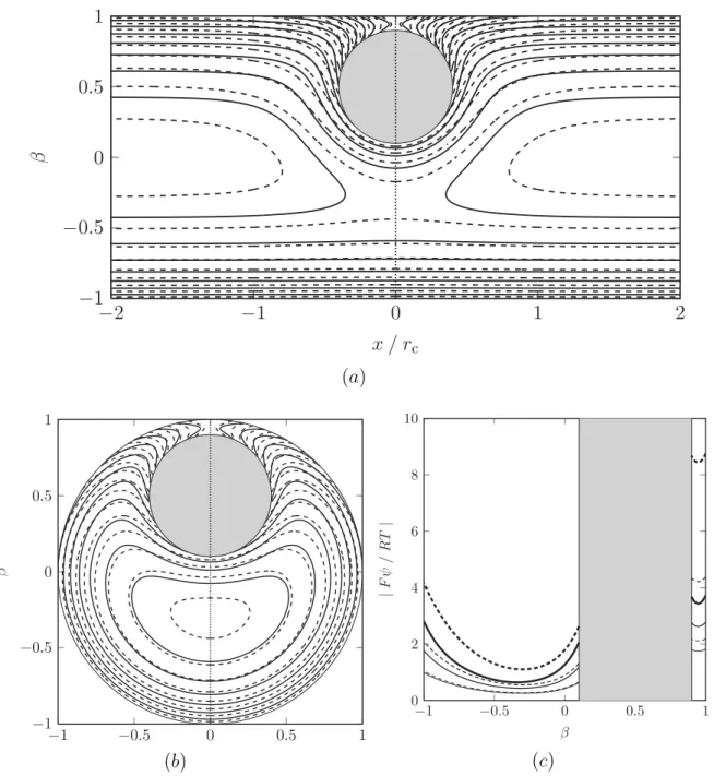
Figure 2. (a) The contours of electrical potential in a longitudinal section of the pore containing the centerline of the pore and the center of a solute, (b) the contours of electrical potential in the cross-section of the pore containing the solute center, and (c) profiles of the electrical potential along the dotted line in figures 2(a) and (b). The parameter values arerc = 10 nm, a= 4 nm, qs =qc = −0.01 C/m², C0 = 0.01 M, and the solute center is placed at β = 0.5. The solid lines represent the results of PB-N, and the dashed lines represent the results of DH-N. The thin and thick lines in figure 2(c) are the corresponding profiles for qs = qc =−0.005 and−0.02 C/m², respectively, with the other parameters unchanged. In figures (a) and (b), the interval between neighboring contours isF∆ψ/RT = 0.2.

0 0.2 0.4 0.6 0

0.2 0.4 0.6 0.8 1

β

exp(−E(β)/kT)

(a)

0 0.2 0.4 0.6

0 0.2 0.4 0.6 0.8 1

β

exp(−E(β)/kT)

(b)

Figure 3. Boltzmann factor exp[−E(β)/kT] as a function of the relative radial position of the solute center for rc = 10 nm, a = 4 nm, at (a) qs = qc = −0.005 C/m² and at (b) qs = qc =−0.02 C/m². The ion concentrations are C0 = 0.01 M (open circles), 0.02 M (squares), 0.04 M (triangles), 0.1 M (diamonds), and 0.15 M (closed circles), corresponding to τ = 3.32, 4.69, 6.63, 10.49 and 12.84, respectively, for aqueous solutions atT = 310 K. The solid lines represent the results of PB-N, the dashed lines represent the results of DH-N, and the dotted lines represent the results of DH-A.

0 0.2 0.4 0.6

0 0.2 0.4 0.6 0.8 1 1.2

β exp[−E(β)/kT]DH/exp[−E(β)/kT]PB

(a)

0 0.2 0.4 0.6

0 0.2 0.4 0.6 0.8 1 1.2

β exp[−E(β)/kT]DH/exp[−E(β)/kT]PB

(b)

Figure 4. Ratios of the Boltzmann factors obtained from the DH equation and the corresponding values obtained from the PB equation, exp[−E(β)/kT]DH−N / exp[−E(β)/kT]PB−N(dashed lines) and exp[−E(β)/kT]DH−A / exp[−E(β)/kT]PB−N

(dotted lines), for rc = 10 nm, a = 4 nm, at (a) qs = qc = −0.005 C/m² and at (b) qs = qc = −0.02 C/m². The ion concentrations are C0 = 0.01 M (open circles), 0.02 M (squares), 0.04 M (triangles), 0.1 M (diamonds), and 0.15 M (closed circles), corresponding to τ = 3.32, 4.69, 6.63, 10.49 and 12.84, respectively, for aqueous solutions atT = 310 K.

3. Results

Figures 2(a) and 2(b) show the contours of the electrical potential for rc = 10 nm, a = 4 nm, qs = qc = −0.01 C/m² and C0 = 0.01 M, with the solute center placed at β = 0.5 from the pore centerline. Profiles of the electrical potential along the dotted line in figures 2(a) and (b) are plotted in figure 2(c). The corresponding profiles for qs =qc=−0.005 C/m² andqs =qc =−0.02 C/m² with the other parameter unchanged are also plotted by thin lines and thick lines, respectively, in figure 2(c). In each figure, the solid lines represent the results of PB-N, and the dashed lines represent the results of DH-N. A strong interaction of the electric double layer formed around the solute and that near the pore wall is seen in figures 2(a) and 2(b). Figures 2(a)-(c) indicate that the magnitudes of the electrical potential obtained from the DH equation are larger than the corresponding values from the PB equation, and the differences between them are significant in the gap region between the solute and the pore wall. Figure 2(c) shows that this difference becomes larger as the magnitude of the charge density is increased.

It can be also shown that the difference is increased with decreasing ion concentration C0 (not shown).

The Boltzmann factor exp[−E(β)/kT] is plotted as a function of the radial position of the solute center for rc = 10 nm, a = 4 nm and C0 = 0.01, 0.02, 0.04, 0.10 and 0.15 M, atqs =qc =−0.005 C/m² in figure 3(a) and at qs =qc=−0.02 C/m² in figure 3(b).

If we define a non-dimensional parameter τ =rc/λD, the cases ofC0 = 0.01, 0.02, 0.04, 0.10 and 0.15 M correspond to τ = 3.32, 4.69, 6.63, 10.49 and 12.84, respectively, for aqueous solutions at T = 310 K. In figures 3(a) and (b), the solid lines represent the results of PB-N, the dashed lines represent the results of DH-N, and the dotted lines represent the results of DH-A. Figures 3(a) and (b) show a decrease in Boltzmann factor as the radial positionβ is increased from 0 to 1−a/rc(= 0.6) for givenτ orτ is deceased for givenβ. The former trend indicates that the solute is more likely to be placed closer to the pore centerline, due to the electrostatic repulsive interaction between the solute and pore charge. The latter trend is because a decrease in τ or an increase in Debye length strengthens the electrostatic interaction, which results in stronger exclusion of solutes from the pore.

It is seen from figures 3(a) and (b) that the results of DH-A and DH- N, exp[−E(β)/kT]DH−A and exp[−E(β)/kT]DH−N, show a good agreement except for the solute placed close to the pore wall, i.e. β ∼ 1 − a/rc, and the values of exp [−E(β)/kT]_DH−A are always larger than the corresponding values of exp [−E(β)/kT]_DH−N. Asβ is increased up to 1−a/rc (= 0.6), the difference between them is more evident in figure 3(a). Although this discrepancy near β ∼ 1−a/rc is invisible in figure 3(b), there is a large relative difference between them in this case as well, which will be seen in figure 4.

In order to show the difference of the Boltzmann factors obtained from the PB equation, exp [−E(β)/kT]_PB−N, and the corresponding values obtained from the DH equation, exp[−E(β)/kT]DH−N and exp [−E(β)/kT]_DH−A, we plotted the

ratios of exp [−E(β)/kT]_DH−N / exp [−E(β)/kT]_PB−N and exp [−E(β)/kT]_DH−A / exp [−E(β)/kT]_PB−N in figure 4, for rc = 10 nm, a = 4 nm and τ = 3.32, 4.69, 6.63, 10.49 and 12.84 at qs =qc =−0.005 and −0.02 C/m². Figures 4(a) and (b) show that the ratio of exp [−E(β)/kT]_DH−N/ exp [−E(β)/kT]_PB−N is always smaller than unity, reflecting the fact that the interaction energy E(β) is overestimated based on the DH equation. It is also seen that the ratio of exp [−E(β)/kT]_DH−N/ exp [−E(β)/kT]_PB−N

decreases monotonically with increasingβ from 0 to 1−a/rcor with decreasing τ. This may be understood from figure 2, which shows large difference in electrical potentials of PB-N and DH-N in the gap region between the solute and the pore wall. This difference is more enhanced for larger β and smaller τ.

In the case of low charge density (qs =qc= −0.005 C/m²), figure 4(a) shows that the ratio of exp [−E(β)/kT]_DH−N / exp [−E(β)/kT]_PB−N remains close to unity for large τ (≥ 4.69 ) over almost the whole range of β except for β ∼ 1−a/rc, while in the case of high charge density (qs = qc = −0.02 C/m²), figure 4(b) shows that the ratio is much smaller than unity for small τ (≤ 6.63) even for the solute placed near the pore centerline. It is interesting to note that the ratio of exp[−E(β)/kT]DH−N / exp[−E(β)/kT]PB−N is as low as about 0.05 forτ = 4.69 and it is nearly 0 forτ= 3.32 in figure 4(b), whereas the Boltzmann factors themselves are visually indistinguishable in both cases, given the linear scale in figure 3(b). This is because the interaction energy E(β)/kT is so large in those cases that the Boltzmann factor exp[−E(β)/kT] is extremely small.

With regard to DH-A, figure 4(a) shows that an increase in β increases the ratio of exp[−E(β)/kT]DH−A / exp[−E(β)/kT]PB−N beyond unity, and the ratio rises rapidly with β approaching (1 − a/rc). The rapid rise of exp[−E(β)/kT]DH−A / exp[−E(β)/kT]PB−N near β ∼ (1− a/rc) is also seen in figure 4(b), indicating that the DH-A underestimates the interaction energy for large β.

Multiplying the Boltzmann factor by β and integrating it over the pore cross- section yields the solute partitioning coefficient Φ (equation (10)). As evident from equations (8) and (9), the quantity Φ represents the ratio of the solute concentration at the pore ends relative to the bulk solution. Figure 5 shows Φ as a function of τ, for rc = 10 nm, a = 2, 4, 6 nm, qs = qc = −0.005 and −0.02 C/m². For small τ, electrostatic effects are so large that solutes are excluded from the pores, while for largeτ, electrostatic effects are unimportant. Thus, each curve increases monotonically with increasing τ and approaches an asymptotic limit corresponding to purely steric exclusion, (1−a/rc)². This limiting value can be easily obtained from equation (10) for E(β) = 0 at 0≤β ≤(1−a/rc).

In general, the difference of Φ values between linear and nonlinear formulations is large for small τ, while it is small for large τ. In the case of low charge density (qs = qc = −0.005 C/m²), open symbols in figures 5(a) and (b) show that the ΦDH−N

values are comparable to those of ΦPB−N and the difference between them becomes noticeable only for small τ. In contrast, the difference between the ΦDH−A values and the ΦPB−N values is evident at low charge density, resulting from that the Boltzmann

4 6 8 10 12 0

0.1 0.2 0.3 0.4 0.5 0.6 0.7

τ(=rc/λD)

Φ

(a)

4 6 8 10 12

0 0.2 0.4 0.6 0.8 1 1.2

τ(=rc/λD) ΦDH/ΦPB

(b)

Figure 5. (a) Partitioning coefficients ΦPB−N (solid lines), ΦDH−N (dashed lines) and ΦDH−A (dotted lines) for rc = 10 nm, qs =qc =−0.005,−0.02 C/m², and (b) ratios of partitioning coefficients obtained from the DH equation and the corresponding values obtained from the PB equation, ΦDH−N/ ΦPB−N(dashed lines) and ΦDH−A / ΦPB−N (dotted lines). The size ratios area/rc = 0.2 (circles), 0.4 (squares), and 0.6 (triangles). Open symbols represent the case ofqs = qc = −0.005 C/m² and closed symbols represent the case ofqs=qc=−0.02 C/m².

factors of DH-A are larger than those of PB-N or DH-N for the solute placed near the pore wall (β ∼ 1−a/rc), as shown in figures 3(a) and 4(a). Figure 5(b) shows that, as τ is increased for given a/rc, the ratio ΦDH−A / ΦPB−N increases from below unity and reaches a maximum at a certain β, beyond which the ratio decreases to approach unity. This behavior is different from the monotonic increase in ΦDH−N / ΦPB−N with increasing τ. At large charge density (qs =qc =−0.02 C/m²), closed symbols in figure 5(b) show that an increase in τ increases both ratios of ΦDH−N / ΦPB−N and ΦDH−A / ΦPB−N monotonically from nearly zero to unity.

By using equations (12) and (13), the hindrance factors H and W were computed, and the obtained results ofH andW are plotted in figures 6 and 7 as functions ofτ, for rc= 10 nm, a = 2, 4, 6 nm, and qs=qc=−0.005 and −0.02 C/m². In the calculation, we adopted the values ofFt and F0 of O-tani et al. (2011). Similarly to the behavior of the partitioning coefficient shown in figure 5, the hindrance factors H and W increase with increasing τ for given a/rc or decreasing charge densities qs, qc for given τ. Their differences between linear and nonlinear formulations also show similar dependence onτ and charge densitiesqs,qc with the partitioning coefficient Φ. In short, the DH-N values ofHand W provide good approximation to the PB-N values at low charge densities and large τ, and an increase in charge densities or a decrease in τ makes the DH-N values smaller compared to the PB-N values. On the other hand, the DH-A values ofH andW are higher than the PB-N values at low charge density (qs=qc=−0.005 C/m²) except

4 6 8 10 12 0

0.1 0.2 0.3 0.4

τ(=rc/λD)

H

(a)

4 6 8 10 12

0 0.2 0.4 0.6 0.8 1 1.2

τ(=rc/λD) HDH/HPB

(b)

Figure 6. (a) Hindrance factors HPB−N (solid lines), HDH−N (dashed lines) and HDH−A (dotted lines) for rc = 10 nm, qs = qc = −0.005, −0.02 C/m², and (b) ratios of hindrance factors obtained from the DH equation and the corresponding values obtained from the PB equation,HDH−N /HPB−N(dashed lines) andHDH−A / HPB−N (dotted lines). The size ratios area/rc = 0.2 (circles), 0.4 (squares), and 0.6 (triangles). Open symbols represent the case ofqs = qc = −0.005 C/m² and closed symbols represent the case ofqs=qc=−0.02 C/m².

4 6 8 10 12

0 0.2 0.4 0.6 0.8

τ(=rc/λD)

W

(a)

4 6 8 10 12

0 0.2 0.4 0.6 0.8 1 1.2

τ(=rc/λD) WDH/WPB

(b)

Figure 7. (a) Hindrance factors WPB−N (solid lines), WDH−N (dashed lines) and WDH−A (dotted lines) for rc = 10 nm, qs = qc = −0.005, −0.02 C/m², and (b) ratios of hindrance factors obtained from the DH equation and the corresponding values obtained from the PB equation,WDH−N / WPB−N (dashed lines) andWDH−A

/WPB−N (dotted lines). The size ratios area/rc= 0.2 (circles), 0.4 (squares), and 0.6 (triangles). Open symbols represent the case ofqs = qc = −0.005 C/m² and closed symbols represent the case ofqs=qc=−0.02 C/m².

τ a/rc

4 6 8 10 12

0.2 0.4 0.6

1

10 10

10 1

0.1 10

10

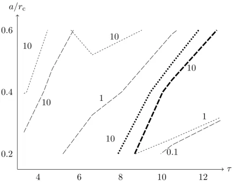
Figure 8. The relative difference of the partition coefficient ∆Φ/ΦPB−N, where ∆Φ represents either|ΦPB−N−ΦDH−A|(dotted lines) or|ΦPB−N−ΦDH−N|(dashed lines) atqs =qc =−0.005 C/m² (thin lines) orqs =qc =−0.02 C/m² (thick lines). Lines show contours of the relative difference and region below and to the right of each line corresponds to the values ofa/r^c andτ at which the relative difference is smaller than the number specified on the line.

for small τ, and lower than the PB-N values at high charge density (qs = qc = −0.02 C/m²).

4. Discussion

For the same configuration with the present study, i.e. a charged spherical solute suspended in an electrolyte solution within a charged circular cylindrical pore, there are pioneering works by Smith & Deen (1980, 1983), which presented analytical expressions for the interaction energy E based on the DH equation. By truncating the series expansion for the interaction energy, Deen and his coworkers calculated approximately the solute partitioning coefficient Φ, the hindrance factorsH, W as well as the osmotic reflection coefficient (Smith & Deen 1980, Smith & Deen 1983, Deen 1987, Bhalla

& Deen 2009, Dechadilok & Deen 2006, Dechadilok & Deen 2009). In a previous study, we adopted the PB equation to estimate the interaction energy and the osmotic reflection coefficient (Akinaga et al. 2008). In a following study, we employed the DH equation to estimate the hindrance factors H and W by a numerical computation O- tani et al. (2011), since the linear DH equation is much easier to solve compared to the nonlinear PB equation.

With regard to the difference between the linear DH and nonlinear PB formulations,