Earnings Management using

Abstract:

Aims: This study investigates the use of other comprehensive income recycling (OCIR) as an earnings management tool for classification shifting under Japanese GAAPand examines whether adopting IFRS prevents earnings management, and tests ‘meeting or beating benchmarks, ‘big bath’ and ‘income smoothing’ hypotheses on whether firms use OCIR to influence current earnings.

Methodology: This study uses regression analysis using a fixed-effect model on a sample of Japanese firms adopting Japanese GAAP(JGAAP) or IFRS.

Findings: A positive association exists between income-increasing OCIR and meeting or beating zero earnings, prior year’s earnings, and managers’ forecasts for JGAAPfirms, but not for IFRS firms, except for meeting or beating prior year’ net income. Moreover, JGAAP(but not IFRS) firms with pre-recycled net income below zero use negative OCIR to reduce current earnings and magnify losses, consistent with the big bath hypothesis. However, there is no evidence for the income smoothing hypothesis. Therefore, permitting OCIR entirely under JGAAP

Earnings Management using

Other Comprehensive Income Recycling:

Evidence from Japan

Shu Inoue

encourages Japanese firms to engage in earnings management using OCIR, while adopting IFRS can prevent this practice.

Keywords: Recycling, Other Comprehensive Income, Earnings Management, Japanese GAAP, IFRS, Meeting or Beating Benchmarks, Big Bath, Income Smoothing

JEL Classification: J33, M41

1. Introduction

Using a Japanese sample, this study investigates whether other comprehensive

income (OCI) recycling is used to shift classification for earnings management

purposes under Japan’ s generally accepted accounting principles (JGAAP) and

International Financial Reporting Standards (IFRS). OCI recycling (OCIR)

substantially differ between JGAAP and IFRS. The Accounting Standards Board of

Japan (ASBJ) accepted the Accounting Standard for Presentation of Comprehensive

Income (ASBJ Statement No. 25) as part of the convergence project between JGAAP

and IFRS in 2010; thus, Japanese listed firms disclose comprehensive income in

addition to net income. However, while JGAAP requires full recycling to emphasise

net income in the income statement, IFRS fundamentally prohibits OCIR due to

earnings management concerns. There is an ongoing debate on whether to prevent

OCI recycling. Historically, the topic of OCIR has been controversial. That OCIR

can be used to manage earnings is a major concern, as expressed by the Financial

Accounting Standards Board (FASB) members (FASB, 1993). Prior literature

provides evidence that eliminating OCIR helps control earnings management (Rees

& Shane, 2012). Previous studies in the United States investigate the opportunistic use of OCIR, focusing on a single industry (e.g., banks or insurance companies) and specific OCI items (Barth et al., 2014; Graham et al., 2005; Lee et al., 2006). By contrast, this study considers earnings management for all recyclable items across industries (except for banks, insurance, and securities companies) in the context of JGAAP.

^１)

Following the research structure of Arthur et al. (2017), I analyse whether OCIR is associated with meeting or beating benchmark measures and whether OCIR is associated with ‘income smoothing’ or ‘big bath behaviour.’ The results are consistent with meeting or beating modelpredictions, indicating that OCIR is used to meet or beat zero earnings, prior year’s earnings, and managers’ forecasts under JGAAP. These results are consistent with those of Graham et al. (2005). However, I do not find significant evidence under IFRS, except for meeting or beating prior year’

net income. Consistent with Barth et al. (2014) and the big bath hypothesis, under JGAAP, I also reveal that managers use income-decreasing OCIR to reflect more losses when a firm’s pre-managed earnings are below zero. Meanwhile, Barth et al.

(2014) find income smoothing behaviour using OCIR in the United States, and so do Arthur et al. (2017) in Australia. However, this study does not obtain significant results about income smoothing, both under JGAAP and IFRS, which is inconsistent with Barth et al. (2014). Moreover, it finds that permitting OCIR entirely under JGAAP encourages Japanese firms to engage in earnings management using OCIR, while adopting IFRS can successfully prevent classification shifting using OCIR.

This study is the first to investigate earnings management using OCIR under JGAAP and IFRS in Japan and has four major contributions. First, unlike previous １) I exclude financial business firms such as banks, securities, insurance, and other financial

firms because they have a substantially different financial reporting framework.

studies investigating a specific industry and a single OCI item, this study provides extensive evidence of the relevance of earnings management to a wide range of OCIR items across different industries. Second, identifying this new type of earnings management method, ‘using OCIR,’ contributes primarily to the literature stream that considers accrual-based and real activity-based approaches as a typical means of earnings management. Specifically, while recycling is basically triggered by actual activities (e.g., selling assets or closing deals), the expected impact is aimed ‘above the line,’ thus shifting OCI to net income from comprehensive income, which is similar to classification shifting. However, some OCI items rely heavily on a manager’s estimation when OCI is to be reclassified, consistent with accrual-based earnings management. OCIR has a mixed nature of earning management forms that are activity-based and accrual-based. Third, I find that OCIR under IFRS is not positively related to earnings management, suggesting that restricting recyclable OCI items under IFRS can prevent earnings management. This finding is relevant to current international debates among standard setters. JGAAP permits all OCI items to be recycled, while IFRS restricts recycling for certain items. For JGAAP, this study supports adopting IFRS, as it provides evidence that JGAAP-based OCIR is used as a means of earnings management. Therefore, Japanese accounting standard setters are encouraged to re-examine the current standard relating to OCIR to eliminate it as a means of earnings management. Meanwhile, the International Accounting Standards Board (IASB) has revised its conceptual framework (IASB 2018), but the current recycling guidance does not provide clear rules on what items should be included in the income statement or the statement of OCI (IASB 2018, par.

7.36). Therefore, future standards need to address this issue. In light of this study’s

finding that OCIR is tend to be used as a method of management’s discretionary

earnings management, and consistent with the IASB’s previous concerns, IASB

should emphasize the need to restrict the existing recycling standard. Finally, the findings here are useful for investors, analysts, and other stakeholders when assessing the performance of firms because using OCIRcan influence the bottom line, and financial statement users are more likely to consider OCIRinformation and make more informed decisions.

2. OCI Regulation and Prior Research

2.1. OCI Regulation in IFRS

In 1997, the International Accounting Standards Committee (IASC) issued IAS 1 Presentation of Financial Statements. The revised IAS 1 in 2003 requires reporting of comprehensive income, and states that OCI should be reported in a statement of total comprehensive income or another OCI statement. In IAS1, OCI is defined as items of income and expenses (including reclassification adjustments) that are not recognised in profit or loss as required or permitted by other IFRSs (IAS1, par.7).

^２)

‘Reclassification adjustments are amount reclassified to profit or loss in the current period that were recognised in other comprehensive income in the current or previous ２) Other comprehensive income includes the following items (IAS1, par. 7), such as (a) changes in revaluation surplus relating to tangible property, plant and equipment, and intangible assets; (b) re-measurement of defined benefit plans for retirement benefits;

(c) gains and losses arising from translating the financial statements of a foreign operation;

(d) gains and losses arising from investments in equity instruments designated at fair value

through other comprehensive income in accordance with paragraph 5. 7. 5 of IFRS 9

Financial Instruments; (d) gains and losses on financial assets measured at fair value through

other comprehensive income in accordance with paragraph 4. 1. 2A of IFRS 9; (e) the

effective portion of gains and losses on hedging instruments in a cash flow hedge; (f) for

particular liabilities designated as at fair value of options when separating the intrinsic value

and time value of an option contract and designating as a hedging instrument only the change

in the intrinsic value; (g) changes in the time value of options; and (h) changes in the value

of forward contracts and changes in the value of foreign currency-based spreads on financial

instruments.

period (IAS1, par.7). ‘Reclassification adjustments’ and ‘recycling’ have the same meaning, but ‘recycling’ is used here because of its familiarity. OCI is basically calculated as the portion of the change in net assets (excluding capital transactions) that is not included in net income during an accounting period. Accounting standards enumerate specific examples of OCI items. OCIR, reported as earnings without the change in net assets, used to be comprehensive income based on the change in net assets in the past. At first recognition, the designated gain or loss in the standard is included as a component of OCI, and when recycled, the gain or loss is included in the earnings that influence net income. OCI includes items that can eventually be transferred to profit or loss and items that cannot be transferred to profit or loss until the end, in accordance with other IFRS provisions. The statement of comprehensive income must show what can and cannot be recycled separately (IAS1, 82A).

OCI items have changed over time. Initially, the mark-to-market difference of

available-for-sales financial assets (AFS) is classified as OCI and then recognised as

profit when profit is realised upon the sale of the financial assets. IAS 1 in the 2003

edition permitted or required the recognition of certain profits directly in equity

(changes in a revaluation surplus (IAS 16) and defined benefit pension plan (IAS

19)), and recycling of OCI (sale of financial assets (IAS 39) and foreign currency

translation (IAS 21)). However, the IASB is critical towards OCIR (IASB, 2005)

because the profit or loss component should be recorded only once in total

comprehensive income. In 2006, the IASB’ s exposure draft of the proposed

amendments to IASB 1 indicated that reclassification would be prohibited (IASB

2006). Since the amendment of IAS 1 in 2007, the IASB has set up a discussion paper

seeking broad comments on whether OCI items should be presented in the income

statement by way of recycling or an OCI statement. Based on these discussions, the

2011 version of IAS 1 allows recycling gains and losses on foreign currency

translation (FX), AFS securities, and cash flow hedges (CFH; IASB2011 IAS1, par.

95), while prohibiting recycling gains and losses on revaluation surplus (REV) and changes and actuarial gains or losses of defined benefit pension plans (DBP;

IASB2011 IAS1, par. 96). Furthermore, the current IFRS 9 Financial Instruments puts more restrictions on OCIR, adding specific AFS to be prohibited. IFRS 9 does not allow OCIR for equity investments financial assets measured at fair value through other comprehensive income (FVTOCI), or where the fair value option has been exercised in any circumstance for a financial asset or financial liability (IASB 2014, IFRS 9, par. 4.4.1). Furthermore, in accordance with IFRS 9, OCIR does not arise if a cash flow hedge or the accounting for the time value of an option results in amounts that are removed from the cash flow hedge reserve or a separate component of equity (IASB2014 IAS1, par. 96). There are major restrictions on the OCI items that can be recycled under IFRS, and they are significantly different from the Japanese standard that insists on fully recycled OCI items with no exceptions. This significant difference in regulations for OCIR leads to expectations that firms applying IFRS will suppress earnings management using OCIR.

2.2. OCI Regulation in JGAAP

Japan has traditionally valued historical accounting system. The conceptual framework issued by ASBJ in 2006 (ASBJ 2006) emphasises that the main component of the financial statement is ‘net income’ (ASBJ 2006, Ch.3 par.18).

Japan emphasises net income because it is the most value-relevant earnings

measurement in the Japanese Conceptual Framework (J-FW) since net income

reflects the result of investments through the realisation concept (ASBJ 2006, Ch1

par.3; Ch.3 par.9). If income is reported before it is realised, this means that the

investment has not produced a result yet, thus conveying uncertain information to

investors about firms’ performance. Regarding the treatment of net income, the concept of earnings realisation still deeply dominates accounting practice in Japan, despite convergence with international accounting standards. This peculiar Japanese accounting philosophy influences the elements of financial statements and the form of the income statement as well. First, comprehensive income (CI) is at the lowest position in J-FW. The purpose of the CIin J-FW is twofold: (1) harmonisation of international FW and (2) its harmlessness. CIin J-FW, provided merely as a supplement to net income, makes J-FW more global on the surface and serves as a potential earnings measurement that may turn out to be useful in the future (ASBJ 2006, Ch.3 par.22). Second, the treatment of OCIrecycling is exceedingly significant in J-FW because of the prominent position of net income. As long as net income is at the highest position in J-FW, OCIrecycling is considered essential for calculating the results of investment adequately through realisation and for keeping the ‘clean- surplus relationship’ between net income and owners’ equity (ASBJ 2006, Ch.1 par.

3, and Ch.3 pars.9,12). Therefore, there is no exceptional OCIrecycling treatment; all OCIitems must be recycled whenever investment is realised.

In 2010, Japan finally accepted the regulation of CI as a GAAP and issued

‘ASBJ Statement No.25 Accounting Standard for Presentation of Comprehensive Income (ASBJ 2010)’. Unlike US GAAP and IFRS, Japan is not very positive in introducing accounting standards for CI, as mentioned in the J-FW above. The purpose of the CIstandard in Japan is to respond to the convergence project (ASBJ 2010, par.20). Furthermore, the position of CIin this standard is to achieve another

‘clean-surplus relationship’ between CIand net assets and provide useful information to users as complementary information to net income (ASBJ 2010, par.21).

Japan’s relentless commitment to full recycling is reflected in the Japanese

version of the revised IFRS. Japan’ s modified IFRS, officially called Japan’ s

Modified International Standards (JMIS), refers to the IFRS in which Japan has some exceptions, mainly the presentation of net income, application of compulsory OCI recycling, and goodwill amortisation.

^３)

Japan claims that OCI recyclingcan consistently represent the cumulative net income and cumulative net cash flow of a firm duringits operatingperiod (ASBJ 2015a). Eventually, OCI recyclingenhances the usefulness of income statement information as an overall indicator of business performance (ASBJ 2015b). Therefore, OCI recyclingis an iconic accounting procedure that reflects the characteristic of Japanese GAAP, that is, ‘net income is the most important accountingmeasurement in the financial statement.’

2.3. Prior Research on OCI Recycling

There is limited empirical research on the relationship between OCIR and earnings management. As an early study, Hirst and Hopkins (1998) show that by clearly displayingcomprehensive income and its components in a separate income statement, earnings management became more transparent for outsiders, which allows analysts to process AFS securities-related information and use it correctly in their valuations. For analysts who are unaware of earnings management using AFS securities, evidence indicates that they overlook lower reportingquality and lower prospects for future performance. However, specific earnings-based benchmarks are not the primary objective of their study. Jones and Smith (2011) argue that managers’

discretion over investment choices and the timing of realisation encourage earnings management concerns regarding OCIR. Graham et al. (2005) conduct a survey in the United States on whether respondents consider the benefits of sellinginvestments

３) Japan insists on goodwill amortisation because it is suitable for the historical cost

accountingsystem and consistent with cost allocation and the matchingprinciple (ASBJ

2003, No.21, par.105).

and other assets to meet or beat prior year’s earnings, and find that 20.2 per cent of CFOs either ‘agree’ or ‘strongly disagree.’ This result indicates that managers are motivated to engage in earnings management using OCIR. Lee et al. (2006) reveal that U. S. insurance company managers engage in ‘cherry-picking’ to timely coordinate the realisation of security gains or losses to manage earnings. Barth et al.

(2014) provide further supporting evidence for this finding. They reveal that U.S.

banks engage in income smoothing and big bath accounting through the sale of AFS securities.

The abovementioned previous studies mainly deal with the sale of AFS financial assets as a means of OCIR. Another relevant area is cash flow hedge accounting. If an asset or liability is recognised as a result of a hedging transaction, the manager has the discretion to recycle once recognized hedge gain or loss as a tool of reclassification adjustment from the OCIstatement to the income statement.

Chiorean et al. (2017) examine whether U. S. firms engage in OCIR earnings

management using cash flow hedge accounting. Their findings reveal that managers

opportunistically reclassify the OCIof cash flow hedge and strategically designate

and de-designate derivatives in cash flow hedges to achieve earnings benchmarks

such as analysts’ forecasts, prior period return on assets (ROA), and zero earnings in

the current period. Furthermore, they find that adopting the revised standard (ASU

2011-05) regarding OCIR does not eliminate earnings management but reduces it

significantly. Arthur et al. (2017), based on a sample of Australian firms, find that

there is a positive link between OCIRs that increase revenue and meeting or

exceeding both last year’ s revenue and analyst forecasts. However, there is no

evidence of using OCIR to avoid losses. In addition, they show that companies whose

OCIR-managed revenues far exceed revenue benchmarks used OCIRs to reduce

revenues. This is consistent with the income smoothing hypothesis. Finally, they

suggest that OCIR and discretionary accrual complement each other rather than compete with each other, providing additional evidence of a significant positive association between OCIR and discretionary accruals.

Rees and Shane (2012) examine whether the demand for OCIR stems from the importance of EPS calculations. If investors emphasise EPS based on net income and OCIR recognizes all realized cumulative transactions through OCI in the net income, EPS will be calculated more favourably than without OCIR (Rees and Shane, 2012).

As long as net income is highlighted in the income statement, OCIR keeps net income a key performance indicator (Detzen, 2016). However, Frendy and Semba (2016) investigate the usefulness of OCI recycling in Japan and reveal that unlike ASBJ’ s expectations that recycling enhances the usefulness of net income, the inclusion of recycling reduces sustainability and increases net income volatility.

3. Hypothesis Development

Following the research structure of Arthur et al. (2017), I analyse whether OCIR is associated with meeting or beating the benchmark measures and whether OCIR is associated with income smoothing or big bath behaviour in the JGAAP context. In addition, I compare IFRS firms to JGAAP firms in terms of whether the strict regulation for OCIR under IFRS can successfully prevent earnings management using OCIR. In accordance with Arthur et al. (2017), I develop hypotheses concerning benchmarks, income smoothing, and big bath accounting.

3.1. Meeting or Beating Zero Earnings

Arthur et al. (2017) state that psychologically, negative numbers are more

difficult to interpret than positive numbers; the natural behaviour of avoiding losses

is explained by human psychological influences (Barrow, 1992; Patel & Zeckhauser, 1999). Past earnings management studies have shown evidence of near-zero discontinuity in the earnings distribution. There are firms with small positive earnings distributed at an unusually high frequency and an unusually low distribution for firms with small negative earnings (e.g., Burgstahler & Dichev, 1997; Degeorge et al., 1999; Hayn, 1995). Hayn (1995) indicates that a significant difference between the observations just above and below zero implies earnings management behaviour that helps to reveal loss-making firms across the ‘red line.’ However, he does not specify exactly how this benchmark can be achieved. Extending this early study, Burgstahler and Dichev (1997), and Degeorge et al. (1999) examine meeting or beating prior-year earnings and analysts’ forecasts as earning-based benchmarks.

They conclude that the main goal of U.S. managers is to meet or beat zero earnings.

In Japan, Suda et al. (2006) investigate earnings distribution and reveal that Japanese firms also engage in earnings management to avoid reducing gains and losses.

Other U.S. studies investigate whether the impact of benchmarks could be due to earnings management. Some studies explain that discontinuities are caused by other factors such as sample selection bias, such as an income scaling mechanism and the effects of income taxes, which indicates that future studies should be considered.

when interpreting the earnings discontinuity in the context of earnings management (Beaver et al., 2007; Durtschi & Easton, 2005). Many previous studies show that managers tend to reach the break-even point using discretionary transitory earnings elements or special items (e.g., Collins et al., 1995; Givoly & Hayn, 1992; Marquardt

& Wiedman, 2004). Marquardt and Wiedman (2004) show that companies that avoid

zero returns tend to be extremely under-reported for unexpected negative special

items. This evidence further suggests that firms treat a special item (i.e., gain or loss

that differs from operating income) as an earnings management tool. Meeting or

beating zero earnings is considered one of the most important earnings-based benchmarks in the accounting literature (Burgstahler & Dichev 1997; Degeorge et al., 1999; Hayn, 1995). Since OCI has the nature of the loss or gain similar to special items, it leads to the following hypothesis that firms realise the gains of OCI items to avoid losses as described above given that OCIR may facilitate managers the opportunity to achieve this benchmark.

H1a: The use of positive OCI recycling increases the likelihood of meeting or beating zero earnings.

3.2. Meeting or Beating Prior Year’s Earnings

Another possible earnings-based benchmark is meeting or beating prior year’s earnings (Burgstahler & Dichev, 1997; Degeorge, Patel, & Zeckhauser, 1999), which is a heuristic cut-off for zero earnings changes and an index that allows a reasonable comparison for management evaluations (Graham et al., 2005; Marquardt &

Wiedman, 2004).Generally, managers believe that if their firm misses targets, the market will punish the firm (Graham et al., 2005). Another evidence reveals that investors are interested in whether managers outperform the previous year’s earnings when assessing firms’ value (Beatty et al., 2002), suggesting capital market incentives.Therefore, managers may engage in earnings management to avoid a negative impact on the company’s stock price.

The concept of OCI is arguably difficult to interpret because of the complexity

associated with an OCI item’ s components, such that nonprofessional investors

generally tend to ignore comprehensive income much less use it (Durocher & Fortin,

2015).Tarca et al.(2008) conduct experiments with financial analysts and

professional accountants as professional users and MBA students as non-

professionals. They obtain evidence that OCIR further complicates OCI descriptions, and non-recycling is easier to understand for all sophisticated levels of users to extract and interpret OCI information. When analysts and investors do not have a clear understanding of OCIR rules and related accounting standards, earnings management behaviour using OCIR is more difficult to detect externally (PwC, 2012). This provides insiders a means for earnings management.

Prior literature shows that compared with private U.S. banks, public U.S. banks are unlikely to report a slight decrease in earnings through the use of public banks’

discretionary provisions for loan loss provisions and the recognition of securities gains and losses (Beatty et al., 2002). This implies that some of the OCI items (AFS securities) could be used to achieve or exceed the prior year’s earnings. There is a relationship between avoiding declines in earnings and OCIR, which leads to the following hypothesis:

H1b: The use of positive OCI recycling increases the likelihood of meeting or beating prior year’s earnings.

3.3. Meeting or Beating Managers’ forecasts

In the United States, researchers use analyst forecasts as earnings-based benchmarks because of their popularity and importance, and studies show that meeting or beating analyst forecasts are important goals (Carvajal et al., 2015; Chu et al., 2015; Herrmann et al., 2011). U. S. managers also use accruals to increase earnings and exceed analyst expectations (Callao & Jarne, 2006; Barua et al., 2015;

Matsumoto, 2002).

In addition to analysts’ forecasts, managers’ forecasts are a mandatory

disclosure for listed firms in Japan. Ota (2002) reveals that in Japan, managers’

forecasts are more valued than analyst’s forecasts. Ota (2011) also shows that analyst forecasts, published after managers’ forecasts, are biased by managers’ forecasts.

Considering the discussion above and the finding that OCIR provides managers with the opportunity to manage earnings, the following hypothesis is proposed:

H1c: Positive OCI recycling increases the likelihood of meeting or beating managers’ forecasts.

3.4. Income Smoothing

While Buckmaster (2001) simply explains that income smoothing occurs when managers what to reduce the volatility of reported earnings using acceptable accounting methods, Fudenberg and Tirole (1995) define income smoothing as ‘the process of manipulating the time profile of earnings or earnings reports to make the reported income stream less variable, while not increasing reported earnings over the long run.’ Earnings smoothness, where managers opportunistically smoothed out reported income to provide a stable earnings stream by allocating intertemporal gains and losses, was once considered a form of earnings management (Beidleman, 1973).

For example, Healy (1985) reveals that managers opportunistically smooth income in an attempt to garble earnings for executive compensation. Several studies document that earnings smoothness is associated with the determinants of low earnings quality such as low-quality country GAAP, less enforcement, or weak shareholder rights (Leuz et al., 2003; Lang et al., 2006; Francis & Wang, 2008). However, investors might consider smoothed earnings as less risky and as facilitating earnings forecasts.

Income smoothing reduces firms’ cost of capital because investors view such firms as having stable returns and lower risk (Graham et al., 2005; Trueman & Titman, 1988).

In addition, analysts and other stakeholders have difficulty in predicting earnings of

firms that have large positive or negative earnings surprises. As such, consistently smoothed earnings trends increase the predictability of firms’ earnings (Kirschenheiter & Melumad, 2002). A smoothed earnings trend is supported by the fact that earnings stability is positively related to the stock price, which leads to an increase in shareholder wealth (Yang & Zhu, 2014). Moreover, previous studies reveal that through income smoothing, managers deliver positive information about a firm’s future earnings; thus, there is a positive relationship between levels of earnings and stock market responses (Davis & Lewis, 1995; Ronen & Sadan, 1981; Tucker &

Zarowin, 2006). Therefore, earnings smoothness signifies earnings quality, assuming that managers achieve representative and useful earnings figures to project future profitability (Francis et al., 2004). Moreover, smoothed earnings can benefit both investors and enterprises if managers want to avoid breaching debt contracts (Carlson

& Bathala, 1997).

Prior research shows that management primarily uses accruals and actual earnings management, but there is some evidence that OCIR is used to manage earnings. Beaver et al. (2003)find that the most profitable firms exaggerate their loss reserves significantly, stating that this provides evidence of income smoothing. Lee et al. (2006)provide evidence that managers in U.S. property-liability insurance firms manage earnings through discretionary realisation of profits or losses on AFS financial assets. Moreover, Barth et al. (2014)report that a sample of U.S.-listed banks engage in income smoothing by increasing the loss of AFS financial assets when pre-managed earnings are sufficiently large. While previous studies focused on specific OCI items (Barth et al., 2014; Lee et al., 2006; Chiorean et al., 2017), I focus on all OCI components from different industries in the Japanese context.

As mentioned above, complexity remains in all components of OCI items,

which creates an opportunity for income smoothing. Following Bath et al. (2014)and

Arthur et al. (2017), this study argues that firms with negative (positive) income managed by OCI realise more profit (loss) in OCI items, as expressed in the following hypothesis:

H2: The level of OCI recycling is negatively related to pre-OCI-managed earnings levels.

3.5. Big Bath Accounting

Kinney and Trezevant (1997) show that when a firm suffers an irreversible loss, the market reaction is not much different from slightly or significantly overlooking the target; therefore, managers prefer to make the loss even worse. The perception is that if the results are poor, worsening the results by ‘cleaning up the table’ does not further harm the firms’ reputation. Firms taking a big bath are likely to achieve significant future earnings growth through ‘inter-period transfer’ (Burgstahler et al., 2002) and restructuring (Cready et al., 2012), with future prospects perceived by investors as low risk. Thus, big bath accounting brings benefits to both firms and managers (Jordan & Clark, 2011). Watts and Zimmerman (1986) also indicate that managers have an incentive to take a big bath to further reduce current earnings during periods when managers are not eligible to receive bonuses, thereby increasing the likelihood of future bonuses. In the long run, pursuing the maximum bonus fits with the firm’s best interests; thus, managers are motivated to engage in earnings management.

Regarding big bath accounting, empirical studies indicate that managers manage earnings through discretionary accruals and real earnings management (Kinney &

Trezevant, 1997; Velury & Kane, 2012). Levitt (1998) states that when a company

decides to reorganise, it typically incurs significant restructuring costs, allowing it to

‘clean up’ its balance sheet. This is also considered a big bath accounting. Jordan and Clark (2011) reveal that SFAS No. 142, which requires yearly testing of goodwill impairment, encourages managers to implement big bath strategies through significant impairment of goodwill. Barth et al. (2014) find evidence that banks with negative earnings realise losses by selling AFS to take a big bath when they do not have enough accumulated unrealised gains that offset negative earnings. Considering the complexity of OCIR, prior literature likely has not sufficiently revealed all OCI items. I expect similar incentives for earnings management across industries when pre-managed income is below zero. Thus, the following hypothesis is proposed:

H3: The level of OCI recycling is positively related to negative pre-OCI- managed earnings.

For the earnings smoothing hypothesis, the relationship between pre-managed earnings and OCIR is expected to be negative, assuming that profits and losses offset each other. For the big bath hypothesis (H3), it is expected to be positive, assuming that the pre-management earnings are negative and the income-decreasing OCIR promotes even larger losses.

3.6. The Effect of Adopting IFRS on OCIR

In a previous study comparing accounting amounts based on IFRS and national

standards, Barth et al. (2008) find that the accounting quality of firms using IFRS in

countries other than the United States is generally higher than that of firms using

local accounting standards. Besides, Barth et al. (2012) also reveal that IFRS

adoption by non-US firms helps improve accounting systems and enhances value

relevance and comparability of reports with US firms. OCIR is strictly restricted

under IFRS, differing in the (1) actuarial gains or loss on defined benefit pension plan (DBP) and (2) equityinvestment financial assets measured at FVTOCI. As such, compared with JGAAP firms, IFRS firms are unlikelyto engage in earnings management using OCIR. The fourth hypothesis is as follows:

H4: IFRS firms do not engage in earnings management using OCI recycling.

4. Research Design

4.1. Models for Meeting or Beating Prior Year’s Earnings

Following Arthur et al. (2017), the basic functional form of meet or beat models to test H1a, 1b, and 1c are as follows:

MBZE

i,t

＝α

0

＋α

1

(D_POCIR)

i,t

＋α

2

Controls

it

＋ε

t

…(1) MBPY

i,t

＝β

0

＋β

1

(D_POCIR)

i,t

＋β

2

Controls

it

＋ ϑ

t

…(2) MBME

i,t

＝γ

0

＋γ

1

(D_POCIR)

i,t

＋γ

2

Controls

it

＋μ

t

…(3)

The analysis using this model assumes that firms are more likely to be involved in earnings management if their earnings are positive (Davis et al., 2007). First, I set a binaryvariable MBZE denoting ‘Meet or Beat Zero Earnings,’ which equals 1 if a firm whose net income scaled bytotal assets at the beginning of the year distributes just above zero and the difference between net income and zero is within five per cent, a ‘suspected’ firm barelyavoiding losses, and is zero otherwise to narrow down the target firms.

Second, to measure whether a firm met or achieved prior year’s profits, this

studysimplyuses as a proxythe difference between current and previous years’

earnings scaled by total assets at the beginning of the year. A change greater than zero (positive sign) signifies meeting or beating prior year’s earnings. I use a binary variable MBPY denoting ‘Meets and Beats Prior Year’s Earnings,’ which equals 1 if the change in earnings divided by total assets is greater than zero and the difference between current earnings and prior earnings is within one per cent, and zero otherwise. Regarding the types of income compared here, JGAAPhas stepwise earnings in the income statement―operating, ordinary, and net income. The impact of recycled earnings differs according to the type of OCI item. DBPinfluences operating income because retirement benefit expenses are operating expenses. AFS, CFH, and OCIR using the equity method for affiliated firms affect ordinary income.

If the gains and losses from OCIR are unusual, they are treated as special items under JGAAP. By contrast, recyclable OCI items under IFRS influence either operating income or net income, depending on the firm because of IFRS flexibility (no specific standard). Therefore, I set operating, ordinary, and net income under JGAAPand operating and net income under IFRS to compare earnings for MBPY.

Third, I use a binary variable MBMF denoting ‘Meets or Beats Managers’

Forecasts,’ which equals 1 when the forecast error is greater than zero and the difference between current earnings and prior earnings is within five per cent, and zero otherwise. Forecast error is calculated as the difference between actual earnings and the latest managers’ earnings forecasts, including operating, ordinary, and net income, and EPS.

^４)

The latest forecasts are the most accurate and often the target of earnings management; the closer they are to the announcement date, the more informative (Habib & Hossain, 2008). Therefore, I use the latest manager’s forecasts.

If a firm’s actual earnings equals or exceeds managers’ forecasts, it is classified into ４) However, there is no ordinary income under IFRS. Operating income, net income, and

EPS are available for IFRS firms in this study.

the ‘Meets or Beats Managers’ Forecasts’ (MBMF) group. In addition, I set various managers’ forecasts for operating, ordinary, and net income, and EPSbecause a variety of managers’ forecasts are available in Japan. Considering the different impacts on stepwise earnings based on the type of OCI items, I compare operating, ordinary, and net income, and EPSas managers’ forecasts.

Because the dependent variables of the meet or beat model are binary (MBZE, MBPY, and MBMF), logistic regression is applied. Using panel data, I implement fixed-effects logistic regression and also include year and industry effects. Using binary independent variables in the said model in the event that firms recognise income-increasing OCI to increase earnings to meet or beat earnings benchmarks, I employ a binary independent variable indicating a positive OCIR (D_POCIR), which equals 1 if OCIR is greater than zero and zero otherwise. Following Arthur et al.

(2017), to test Hypotheses 1a, 1b, and 1c, the following logistic regressions are estimated:

MBZE

i,t

＝α

0

＋α

1

(D_POCIR)

i,t

＋α

2

BTM

i,t

＋α

3

SIZE

i,t

＋α

4

LEV

i,t

＋α

5

∆ OCF

i,t

＋α

6

VOL

i,t

＋α

7

ACMOCI

i,t

＋ε

t

…(1) MBPY

i,t

＝β

0

＋β

1

(D_POCIR)

i,t

＋β

2

BTM

i,t

＋β

3

SIZE

i,t

＋ β

4

LEV

i,t

＋β

5

∆ OCF

i,t

＋β

6

VOL

i,t

＋ β

7

ACMOCI

i,t

＋ ϑ

t

…(2) MBME

i,t

＝γ

0

＋γ

1

(D_POCIR)

i,t

＋γ

2

MB

i,t

＋γ

3

SIZE

i,t

＋γ

4

LEV

i,t

＋γ

5

∆ OCF

i,t

＋γ

6

VOL

i,t

＋γ

7

ACMOCI

i,t

＋μ

t

…(3)

The dependent variable, MBPY, basically compares net income (MBPY_NI)

under both JGAAP and IFRS. I also use various dependent variables, including

operating income (MBPY_OP) and ordinary income (MBPY_OR) under JGAAP, and

MBPY_OP under IFRSbecause the impact of recycled earnings differs based on the

type of OCI items. Similarly, the dependent variable, MBME, also includes net income (MBME_NI), operating income (MBME_OP), ordinary income (MBME_

OR), and EPS (MBME_EPS) under JGAAP, or MBME_NI, MBME_OP, and MBME_

EPS under IFRS. Proxies used in this study for controlling other earnings management opportunities include book to market ratio (BTM), firm size (SIZE), change of operating cash flow ( ΔOCF), leverage (LEV), market volatility (VOL), and accumulated OCI beginning of the year (ACMOCI).

The book to market ratio (BTM) controls for the firm’s growth opportunities, which may affect earnings management behaviour (Skinner & Sloan, 2002; Gunny, 2010; Bartov et al., 2002). To control for political costs, I use the control variable SIZE, which is measured as the natural log of a company’s market capitalisation at the beginning of the year (Watts & Zimmerman, 1978; Gunny, 2010; Payne, 2008).

The natural log of market capitalisation is used to remove any skewness that may be associated with a firm’s market value. Leverage (LEV) is set based on previous findings that firms have incentives to manage earnings to avoid debt violations and deterioration of debt ratings (Bowen et al., 2008). Another study also suggests that highly leveraged firms are likely to meet or beat analyst expectations (Davis et al., 2007). The change of operating cash flow ( ΔOCF) measurements are included in the meet or beat model based on the significant relationship between high cash flow levels and earnings management opportunities (Bowen et al., 2008; Minutti-Meza, 2013). Market volatility (VOL) is a measure of volatility with regard to firm and asset values, calculated as the average annual price movement from average to high and low. Prior research indicates that the higher the volatility, the more difficult it is for managers to predict future performance (e.g., Lim, 2001; Duru and Reeb, 2002;

Givoly et al., 2009). Therefore, higher volatility representing a higher risk in a firm

may increase the probability of earnings management. Finally, since OCI items are

initially retained in the statement of financial position as cumulative OCI and then classified as earnings after recycling, firms with large accumulated OCI have a better chance of using OCIR to achieve benchmarks. Therefore, the amount of OCI accumulated at the beginning of the year (ACMOCI)is expected to be positively related to meeting or beating the benchmarks in this context.

I perform hypothesis testing using three meet or beat models: zero earnings, prior year earnings, and managers’ forecasts. The dependent variable represents firms that achieve or miss various benchmarks. If the coefficient of D_OCIP (α 1, β 1, γ 1) is positive and significant, this indicates that income-increasing OCIR is associated with meeting or beating benchmarks, supporting hypotheses 1a to 1c.

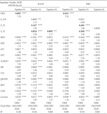
4.2. Models for Income Smoothing and Big Bath Accounting

Bath et al. (2014)argues that when net income is negatively related to realised gains or losses on AFS securities, evidence indicates that income smoothing is conducted. Following Bath et al. (2014)and Arthur et al. (2017), I test the income smoothing hypothesis by examining the relationship between OCIR and net income before OCIR. Previous studies, such as Walsh (1991), Kirschenheiter and Melumad (2002), and Jordan and Clark (2011) show that big baths tend to happen throughout the year and reduce earnings. Therefore, investigating the relationship between OCIR and negative net income before OCIR enables me to consider whether the manager adopts big bath accounting with negative OCIR. The fixed effect regressions (testing H2 and H3)to be estimated and employed are as follows:

OCIR

i,t

＝δ

0

＋δ

1

PTNI

i,t

＋δ

2

IROA

i,t

＋δ

3

SIZE

i,t

＋δ

4

LEV

i,t

＋δ

5

OCF

i,t

＋δ

6

ACMOCI

i,t

＋δ

7

MB

i,t

＋δ

8

TAX

i,t

＋δ

9

QRATIO

i,t

＋δ

10

RED

i,t

＋δ

11

COM

i,t

＋τ

t

…(4)

OCIR

i,t

＝θ

0

＋θ

1

D_PNI

i,t

＋θ

2

P_NI

i,t

＋θ

3

N_NI

i,t

＋θ

4

IROA

i,t

＋θ

5

SIZE

i,t

＋θ

6

LEV

i,t

＋θ

7

OCF

i,t

＋θ

8

ACMOCI

i,t

＋θ

9

MB

i,t

＋θ

10

TAX

i,t

＋θ

11

QRATIO

i,t

＋θ

12

RED

i,t

＋θ

13

COM

i,t

＋φ

t

…(5) NOCIR

i,t

＝ρ

0

＋ρ

1

N_NI

i,t

＋ρ

2

IROA

i,t

＋ρ

5

SIZE

i,t

＋ρ

6

LEV

i,t

＋ρ

7

OCF

i,t

＋ρ

8

ACMOCI

i,t

＋ρ

9

MB

i,t

＋ρ

10

TAX

i,t

＋ρ

11

QRATIO

i,t

＋ρ

12

RED

i,t

＋ρ

13

COM

i,t

＋ω

t

…(6)

These models refer to Arthur et al. (2017). As the dependent variables in the income smoothing and big bath models are continuous variables, fixed effect regressions are implemented on a pooled sample because the individuality of each firm is completely eliminated in the calculation of the fixed effect estimation in the case of pooling regression analysis using panel data. To avoid mechanical correlations between pre-recycled net income (PRNI) and ROA, I use the difference between the firm’s ROA and adjusted ROA by its industry median (IROA). The median of industry returns on assets, which measures the profitability of the industry to which a firm belongs, is included to control for industry-specific performance and macroeconomic factors, and it is a proxy for the average profitability of firms. Bartov et al. (2002) and Minutti-Meza (2013) show a significant relationship between higher ROA and meeting or beating analysts’ forecasts. For the meet and beat models above, I designate leverage (LEV), operating cash flow (OCF), market to book ratio (MB), firm size (SIZE), and accumulated OCI at the beginning of the year (ACMOCI) as control variables. Besides, I also include a quick ratio (QRATIO) as a control variable based on the evidence regarding financial structure and liquidity that there is a significant and positive relation between firm liquidity and OCIR (Barth et al., 2014).

I set tax expenses (TAX) to control for tax incentives because managers might sell

assets to reduce tax expenses. Dividends from retained earnings (RED) and

management compensation (COM) are included to control both motivations because OCIR increases current net income.

In Equation (4), the sign of the coefficient on PRNI is predicted to be negative if supporting income smoothing or positive if supporting the big bath hypothesis.

Equation (5) simultaneouslytests the earnings smoothing (H2) and big bath (H3) hypotheses, focusing on the coefficients for positive and negative pre-management earnings, respectively. A significant negative coefficient for P_NI means that the OCIR signs are contraryto the pre-management income and offset each other’s earnings, therebysupporting the income smoothing hypothesis (H2). Meanwhile, a positive significant coefficient of N_NI means that the OCIR is positivelyassociated with negative net income, therebysupporting the big bath hypothesis (H3). Equation (6) is modeled specificallyto test directlybig bath behaviour using negative PRNI and income-decreasing OCIR, expecting coefficient ρ

1

to be positive to support H3.

All variables (see Appendix A) are scaled bythe total assets at the beginning of the year (except for indicator variables) and winsorized byindustryat the one and 99 per cent levels to minimise the influence of anypotential outliers. The estimated coefficients for each variable are robust t-statistics based on standard errors clustered at the firm level and fiscal year. Since I use panel data in this study, controlling for fixed effects is crucial. The year- and industry-fixed effects are included in the results. To control for firm-specific effects, the ‘Hausman test’ is necessary (Hausman et al., 1981). This test is undertaken to establish which model between a random effect model and a fixed-effects model is more suitable for the panel data.

The result of the Hausman test favours the fixed effects model; thus, it is adopted in

the panel datasets to deal with correlated omitted variables.

^５)

5. Sample Selection Descriptive Statistics

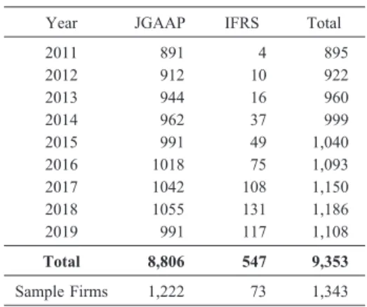
My sample consists of 9,353 firm-year observations representing 1,343 firms that adopt JGAAPor IFRS from 2011 to 2019 in Japan because Japan has adopted the OCI accounting standard under JGAAPsince 2011. I use the NEEDS- FinancialQUEST Nikkei databases to obtain financial statement data. I exclude financial business firms such as banks, securities, insurance, and other financial firms because they have a substantially different financial reporting framework. I delete observations whose fiscal periods are not equal to twelve months and observations with missing data. I also drop the firm-observation whose accumulated OCI on the financial position statement at the beginning of the year is zero because there is no chance to reclassify OCI items without it. Moreover, firm size can affect the quality of earnings (Ball & Foster, 1982; Doyle et al., 2007). Therefore, firms that apply IFRS are considered to be relatively large; thus, firms with total assets of less than 500 million USD are deleted in this study. In the sample, 8,806 observations (1,222 firms) are JGAAPfirms, and 547 observations (73 firms) are IFRS firms. Table 1 provides the sample selection. Table 2 presents the composition of the industry classification based on the Nikkei-Middle-Industry Classification codes.

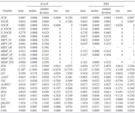
Table 3 shows the descriptive statistics for each of the JGAAPand IFRS explanatory variables, including mean, median, standard deviation, minimum, and maximum. The mean MBZE is 0.1006 under JGAAP(0.0475 under IFRS), implying that firms adopting under JGAAPare more densely distributed near-zero earnings.

５) The greatest merit of the fixed-effect model is that the individual (firm) effect, which

cannot be made a variable, does not affect the estimated value because the individuality of

each firm is completely eliminated in the calculation of the fixed effect estimation. In

pooling regression analysis using panel data, the estimates are far from appropriate because

the unobserved heterogeneity biases the estimates.

Table 1: Sample selection

Year JGAAP IFRS Total

2011 891 4 895

2012 912 10 922

2013 944 16 960

2014 962 37 999

2015 991 49 1,040

2016 1018 75 1,093

2017 1042 108 1,150

2018 1055 131 1,186

2019 991 117 1,108

Total 8,806 547 9,353

Sample Firms1,222 73 1,343

Table 2: Industrycomposition

Industry JGAAP IFRS Industry JGAAP IFRS

Food 393 26 Fisheries 37

Fiber 140 Mining 32

Pulp and paper 86 Construction 621

Chemicals720 42 Trading 847 44

Medical supplies 185 39 Retailer 759 17

Oil 42 4 Other financial services 194 8

Rubber 74 11 Real estate 268 11

Glass and ceramic 167 13 Rail and bus 214

Steel industry 171 6 Land transportation 144 9

Metal products314 11 Sea trans portation 63

Machinery 698 33 Air transportation 24

Electrical equipment 692 81 Warehouse transportation 101

Shipbuilding 33 Communication 108 13

Automobile 367 69 Electric 47

Transportation equipment 81 Gas 77

Precision machine 118 21 Service 721 89

Other manufacturing industries 268 Total 8,806 547

The mean of meeting or beating prior-year (MBPY) for stepwise earnings between under JGAAP and IFRS is similar, implying both standards firms are interested in the prior earnings as benchmarks. The higher ratio of meeting or beating managers’

forecasts under IFRS indicates that it is more sensitive benchmarks for IFRS firms to meet or beat managers’ forecasts due to the global firms. The average of OCIR under IFRS is higher than JGAAP indicates that firms under IFRS have more opportunity to reclassify OIC items even with the OCIR restrictions under IFRS. The mean of D_

OCIP is 0.3924 under JGAAP (0.3144 under IFRS), which implies that 40 per cent (32 per cent) of firm-year observations use positive OCIR. The difference between

Table 3: Descriptive statistics

JGAAP IFRS

Variables mean median standard deviation min. max. mean median standard deviation min. max.

OCIR 0.0007 0.0000 0.0044 −0.0400 0.1284 0.0010 0.0000 0.0065 −0.0184 0.0867 POCIR 0.0010 0.0000 0.0040 0 0.1284 0.0013 0.0000 0.0063 0 0.0867 NOCIR −0.0003 0.0000 0.0016 −0.0400 0 −0.0003 0.0000 0.0012 −0.0184 0 D_POCIR 0.3925 0.0000 0.4883 0 1 0.3144 0.0000 0.4647 0 1 D_NOCIR 0.2178 0.0000 0.4128 0 1 0.2742 0.0000 0.4465 0 1

MBZE 0.1006 0.0000 0.3008 0 1 0.0475 0.0000 0.2130 0 1

MBPY_NI 0.0604 0.0000 0.2383 0 1 0.0622 0.0000 0.2417 0 1 MBPY_OP 0.0402 0.0000 0.1964 0 1 0.0347 0.0000 0.1833 0 1

MBPY_OR 0.0376 0.0000 0.1902 0 1 − − − − −

MBMF_NI 0.1012 0.0000 0.3016 0 1 0.1353 0.0000 0.3423 0 1 MBMF_OP 0.1304 0.0000 0.3367 0 1 0.1627 0.0000 0.3694 0 1

MBMF_OR 0.1175 0.0000 0.3221 0 1 − − − − −

MBMF_EPS 0.0968 0.0000 0.2956 0 1 0.1261 0.0000 0.3323 0 1

BTM 1.1123 1.0135 0.5949 0.0814 6.0255 0.8054 0.7357 0.4878 0.0814 3.2434

SIZE 12.1887 11.9045 1.0668 10.8270 16.7570 13.2347 13.2680 1.5735 8.3180 16.8720

LEV 0.5209 0.5178 0.2050 0.0258 1.9289 0.5410 0.5187 0.2145 0.0658 1.9289

ΔOCF −0.0019 −0.0013 0.0504 −0.3174 0.3441 −0.0025 −0.0022 0.0403 −0.1966 0.1525

VOL 0.1117 0.0584 0.3353 −0.7020 4.5499 0.0988 0.0325 0.3932 −0.5799 2.2913

ACMOCI 0.0146 0.0071 0.0418 −0.1373 0.5224 0.0171 0.0122 0.0427 −0.1116 0.1935

PRNI 0.0361 0.0326 0.0325 −0.1307 0.2448 0.0510 0.0452 0.0434 −0.1151 0.2448

IROA 0.0019 −0.0003 0.0300 −0.1533 0.2152 0.0091 0.0034 0.0413 −0.1601 0.2152

OCF 0.0654 0.0651 0.0498 −0.3824 0.3189 0.0850 0.0848 0.0524 −0.1126 0.3189

TAX 0.0197 0.0163 0.0153 −0.0013 0.2026 0.0230 0.0186 0.0193 0.0000 0.1681

QRATIO 1.5876 1.2726 1.3242 0.0903 23.7058 1.5474 1.2993 1.0512 0.3184 8.3187

RED 0.0108 0.0087 0.0088 0.0000 0.0785 0.0159 0.0131 0.0121 0.0000 0.0785

COM 0.0008 0.0001 0.0016 0.0000 0.0160 0.0018 0.0009 0.0033 0.0000 0.0250

There are 9,353 firm-year observations. All variables are winsorized at 1 percent and 99 percent. See variable definitions in Appendix A.

the median of industry ROA and firm ROA (IROA), MB, and OCF show that the observed sample has positive profitability, higher market price compared to book value, and positive cash cash flows on average consistent to Arthur et al. (2017).

Before showing the results of the regressions, the Pearson correlation matrix for the dependent and explanatory variables is reported in Table 4. Panel A shows variables under the hypothesis 1a to 1c while Panel B under the hypothesis 2 and 3.

The upper (lower) row presents a Pearson correlation matrix under IFRS (JGAAP). I test the variance inflation factor (VIF) as an index to detect multicollinearity between independent variables. The VIF in all models is less than 10, suggesting that there is no collinearity problem.

6. Regression Results

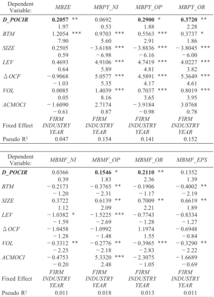
The following sections report and analyse the results of the fixed-effect regression for testing the hypotheses. Table 5 presents the results of the fixed-effect logit regression for the meet or beat hypotheses (H1a to H1c). Panel A (B) presents JGAAP (IFRS). Additionally, Table 6 indicates the results of the fixed-effect regressions for the income smoothing and big bath hypotheses (H2 and H3) under both JGAAP and IFRS.

H1a, H1b, and H1c propose that income-increasing OCIR is used by managers

to achieve earnings benchmarks. Hypotheses 1a, 1b, and 1c are supported if the

coefficient for dummy independent variables, D_POCI, is positive, as firms with

positive OCIR are more likely to achieve earnings benchmarks. Except for regarding

net income benchmarks such as MBPY_NI, MBMF_NI, and MBMF_EPS under

JGAAP, the results show that all coefficients for D_POCI are positively significant

under JGAAP, supporting hypotheses 1a, 1b, and 1c. Meanwhile, there is no

Table 4: Pearson correlation matrix (Upper row IFRS; Lower rowJGAAP) Panel A: Benchmark Hypothesis JGAAP/IFRS OCIR D_POCIR D_NOCIR MBZE MBPY_NI MBPY_OP MBPY_OR M BMF_NI MBMF_OP MBMF_OR MBMF_EPS BTM SIZE LEV Δ OCF VOL ACMOCI OCIR 1 0.331 − 0.197 − 0.037 0.009 − 0.038 − 0.018 − 0.057 0.042 0.036 − 0.045 − 0.125 0.025 − 0.016 − 0.085 0.051 0.079 D_POCIR 0.358 1 − 0.416 0.071 0.054 − 0.043 − 0.024 0.008 0.022 − 0.043 0.039 − 0.087 0.190 0.019 − 0.028 0.071 0.116 D_NOCIR − 0.265 − 0.424 1 0.036 − 0.023 0.040 − 0.006 0.068 0.029 0.013 0.038 0.000 0.221 0.057 0.014 − 0.062 − 0.040 MBZE 0.019 0.017 − 0.006 1 0.120 0.052 0.082 − 0.038 − 0.075 − 0.053 − 0.033 0.154 0.026 0.149 0.011 − 0.072 0.024 MBPY_NI − 0.003 − 0.022 0.005 0.101 1 0.241 0.738 − 0.013 − 0.073 − 0.044 − 0.029 0.124 − 0.041 0.155 0.092 0.088 − 0.090 MBPY_OP 0.000 − 0.017 − 0.013 0.057 0.453 1 0.358 0.100 0.052 0.058 0.078 0.061 0.009 0.055 0.066 0.050 0.003 MBPY_OR − 0.002 − 0.019 − 0.018 0.069 0.504 0.634 1 0.024 − 0.043 0.011 0.003 0.103 − 0.046 0.129 0.082 0.033 − 0.024 MBMF_NI − 0.002 0.017 − 0.008 − 0.030 − 0.014 0.006 0.013 1 0.231 0.331 0.896 − 0.098 0.082 − 0.002 0.041 0.048 − 0.031 MBMF_OP 0.014 0.036 − 0.009 − 0.045 − 0.030 − 0.023 − 0.009 0.224 1 0.467 0.220 − 0.164 0.011 − 0.032 − 0.029 0.047 − 0.035 MBMF_OR − 0.004 0.027 − 0.028 − 0.045 − 0.017 − 0.005 0.000 0.287 0.442 1 0.298 − 0.143 − 0.054 − 0.054 0.014 0.029 0.008 MBMF_EPS − 0.003 0.024 − 0.015 − 0.028 − 0.017 0.007 0.012 0.894 0.210 0.274 1 − 0.092 0.081 − 0.017 0.059 0.043 − 0.055 BTM − 0.050 − 0.100 0.038 0.155 0.094 0.069 0.063 − 0.076 − 0.112 − 0.079 − 0.074 1 0.007 0.036 − 0.016 − 0.312 − 0.016 SIZE 0.012 0.160 0.110 0.034 − 0.021 − 0.005 − 0.011 0.050 0.067 0.043 0.051 − 0.229 1 0.200 0.014 − 0.037 0.169 LEV − 0.037 0.015 0.063 0.159 0.071 0.059 0.049 − 0.027 − 0.020 − 0.027 − 0.023 − 0.058 0.258 1 0.006 0.155 − 0.197 Δ OCF − 0.001 0.000 0.012 − 0.019 0.077 0.061 0.065 − 0.010 − 0.013 0.013 − 0.005 − 0.025 − 0.007 0.009 1 0.148 − 0.003 VOL − 0.014 0.036 0.022 − 0.071 0.063 0.017 0.025 − 0.012 0.005 − 0.005 − 0.004 − 0.299 − 0.010 0.098 0.111 1 − 0.068 ACMOCI 0.168 0.141 − 0.081 0.046 − 0.049 − 0.030 − 0.033 − 0.004 0.009 − 0.017 − 0.002 − 0.084 − 0.025 − 0.052 0.003 − 0.053 1

Thereare9,353firm-yearobservations.Allvariablesarewinsorizedat1percentand99percent.SeevariabledefinitionsinAppendixA.

Panel B: Income smoothing and Big bath Hypothesis JGAAP/IFRS OCIR POCIR NOCIR PRNI P_NI N_NI IROA SIZE LEV OCF ACMOCI BTM TAX QRATIO RED COM OCIR 1 0.983 0.233 0.230 0.255 0.017 0.123 0.025 − 0.016 − 0.001 0.079 0.188 0.186 0.070 0.159 − 0.024 POCIR 0.933 1 0.050 0.221 0.244 0.022 0.120 0.032 − 0.006 − 0.002 0.075 0.197 0.187 0.063 0.161 − 0.029 NOCIR 0.410 0.053 1 0.081 0.093 − 0.024 0.033 − 0.033 − 0.055 0.005 0.030 − 0.020 0.023 0.052 0.013 0.019 PRNI 0.152 0.133 0.084 1 0.952 0.427 0.966 − 0.108 − 0.344 0.625 0.004 0.416 0.737 0.284 0.646 0.159 P_NI 0.160 0.151 0.063 0.923 1 0.187 0.925 − 0.166 − 0.353 0.606 − 0.021 0.463 0.786 0.319 0.652 0.224 N_NI 0.011 − 0.011 0.059 0.459 0.191 1 0.429 0.160 0.020 0.253 0.109 − 0.008 0.113 − 0.125 0.163 − 0.117 IROA − 0.008 − 0.011 0.007 0.918 0.841 0.451 1 − 0.060 − 0.282 0.602 − 0.025 0.360 0.709 0.242 0.583 0.134 SIZE 0.012 0.024 − 0.028 − 0.044 − 0.042 − 0.001 0.006 1 0.200 − 0.081 0.169 − 0.229 − 0.242 − 0.235 − 0.044 − 0.674 LEV − 0.037 − 0.037 − 0.009 − 0.310 − 0.313 − 0.053 − 0.220 0.258 1 − 0.423 − 0.197 0.053 − 0.322 − 0.534 − 0.367 − 0.057 OCF − 0.010 − 0.011 − 0.039 0.468 0.466 0.153 0.430 0.004 − 0.245 1 − 0.003 0.279 0.585 0.211 0.429 0.040 ACMOCI 0.168 0.153 0.078 − 0.014 − 0.031 0.030 − 0.085 − 0.025 − 0.052 − 0.084 1 − 0.042 − 0.043 0.184 − 0.063 − 0.117 BTM 0.042 0.043 0.008 0.398 0.427 0.028 0.346 0.150 0.069 0.304 0.076 1 0.460 0.123 0.375 0.293 TAX 0.044 0.041 0.019 0.714 0.738 0.126 0.662 − 0.060 − 0.299 0.474 − 0.108 0.401 1 0.269 0.581 0.213 QRATIO − 0.002 − 0.003 0.001 0.214 0.224 0.013 0.167 − 0.125 − 0.601 0.055 − 0.033 0.021 0.182 1 0.271 0.180 RED 0.048 0.050 0.007 0.643 0.660 0.123 0.557 − 0.045 − 0.464 0.396 − 0.096 0.437 0.630 0.355 1 0.105 COM 0.007 0.008 − 0.001 0.096 0.094 0.024 0.087 − 0.252 − 0.048 0.053 − 0.036 0.007 0.138 0.031 0.093 1.000

Thereare9,353firm-yearobservations.Allvariablesarewinsorizedat1percentand99percent.SeevariabledefinitionsinAppendixA.

Table 5: Fixed effects logistic regressions of Meet and Beat benchmarks Test Panel A: JGAAP Firms

Dependent

Variable: MBZE MBPY_NI MBPY_OP MBPY_OR

D_POCIR 0.2057

^＊＊

0.0692 0.2900

^＊

0.3720

^＊＊

1.97 0.53 1.88 2.28

BTM 1.2054

^＊＊＊

0.9703

^＊＊＊

0.5563

^＊＊＊

0.3737

^＊

7.90 5.60 2.91 1.86

SIZE 0.2505 −3.6188

^＊＊＊

−3.8836

^＊＊＊

−3.8045

^＊＊＊

0.59 −6.98 −6.16 −6.00

LEV 0.4693 4.9106

^＊＊＊

4.7419

^＊＊＊

4.0227

^＊＊＊

0.64 5.89 4.81 3.82

ΔOCF −0.9068 5.0577

^＊＊＊

4.5891

^＊＊＊

5.3649

^＊＊＊

−1.03 5.35 4.17 4.61

VOL 0.0085 1.4039

^＊＊＊

0.7037

^＊＊＊

0.8019

^＊＊＊

0.05 8.16 3.65 3.95

ACMOCI −1.6090 2.7174 −3.9184 3.0768

−0.61 0.87 −0.98 0.78

Fixed Effect FIRM INDUSTRY

YEAR

INDUSTRY FIRM YEAR

INDUSTRY FIRM YEAR

INDUSTRY FIRM

Pseudo R

²

0.047 0.154 0.141 YEAR 0.152

Dependent

Variable: MBMF_NI MBMF_OP MBMF_OR MBMF_EPS

D_POCIR 0.0366 0.1546

^＊

0.2110

^＊＊

0.1352

0.39 1.83 2.36 1.39

BTM −0.2173 −0.3765

^＊＊

−0.1906 −0.4002

^＊＊

−1.20 −2.31 −1.17 −2.19

SIZE 0.3722 0.6139

^＊＊

0.7009

^＊＊

0.6619

^＊＊

1.12 2.09 2.21 1.89

LEV −1.0382

^＊

−1.5225

^＊＊＊

−0.7743 −0.8334

−1.59 −2.69 −1.28 −1.27

ΔOCF −1.0458 −1.0992 1.1974 −0.6948

−1.28 −1.48 1.55 −0.84

VOL −0.3312

^＊＊

−0.2776

^＊＊

−0.3965

^＊＊＊

−0.3290

^＊＊

−2.25 −2.18 −2.83 −2.22

ACMOCI −0.4753 5.3320

^＊＊＊

−2.3075 −1.6689

−0.20 2.48 −1.05 −0.69

Fixed Effect FIRM INDUSTRY

YEAR

INDUSTRY FIRM YEAR

INDUSTRY FIRM YEAR

INDUSTRY FIRM YEAR

Pseudo R

²

0.011 0.018 0.013 0.011

This table presents the results of H1a-H1c using fixed effect logit model regressions.

＊＊＊

,

^＊＊

,

^＊

indicate two-sided statistical significance at the 0.01, 0.05, and 0.10 levels, respectively.

Robust p-value of the coefficients for all variables are two tailed reported in parentheses.

All variablesare defined in Appendix

Panel B: IFRS Firms Dependent

Variable: MBZE MBPY_NI MBPY_OP

D_POCIR −0.1520 1.6455

^＊＊

−1.3230

−0.17 1.92 −1.08

BTM 3.8533

^＊

0.7229 1.4811

1.68 0.76 0.29

SIZE 1.7684 −1.3388 −4.8590

^＊＊

0.25 −0.45 −2.16

LEV −3.8517 2.2890 −7.1604

−1.11 0.86 −0.87

ΔOCF −6.1441 11.5301

^＊

8.5105

−0.63 1.83 0.99

VOL 0.9239 0.9582 6.0642

^＊

0.53 1.50 1.80

ACMOCI 5.6211

^＊

−2.3771 2.7135

1.65 −1.12 0.14

Fixed Effect FIRM INDUSTRY

YEAR

INDUSTRY FIRM YEAR

INDUSTRY FIRM

Pseudo R

²

0.156 0.050 YEAR 0.048

Dependent

Variable: MBMF_NI MBMF_OP MBMF_EPS

D_POCIR 0.2794 −0.0062 0.4664

0.68 −0.02 1.10

BTM −2.9909

^＊＊

−1.2621 −3.9233

^＊＊＊

−2.29 −1.39 −2.69

SIZE 0.3500 0.2946 0.4507

0.24 0.22 0.31

LEV 0.1547 2.2679 −0.5517

0.07 1.21 −0.22

ΔOCF 2.5644 −2.6117 4.6272

0.68 −0.72 1.18

VOL −0.3395 −0.1418 −0.6797

−0.58 −0.30 −1.21

ACMOCI −8.7586 1.8386 −9.0170

−1.12 0.32 −1.08

Fixed Effect FIRM INDUSTRY

YEAR

INDUSTRY FIRM YEAR

INDUSTRY FIRM YEAR

Pseudo R

²

0.041 0.081 0.076

Thistable presentsthe resultsof H1a-H1c using fixed effect logit model regressions.

＊＊＊

,

^＊＊

,

^＊

indicate two-sided statistical significance at the 0.01, 0.05, and 0.10

levels, respectively. Robust p-value of the coefficients for all variables are two

tailed reported in parentheses. All variables are defined in Appendix A.

significant result under IFRS, except for meeting or beating prior year net income (MBPY_NI), suggesting that the results are not sufficient to confirm the hypotheses under IFRS.

H2 proposes that OCIR is related to earnings smoothing behaviour, assuming that profitable firms recognise income-decreasing OCIR and intentionally reduce their earnings. By contrast, loss-making firms recognise income-increasing OCIR and increase their earnings. Therefore, H2 is supported when the coefficient on PRNI in Equation (4) is negative and significant. H2 is also supported when the coefficient of P_NI or N_NI in Equation (5) is negative and significant.

Similarly, H3 proposes that OCIR is related to big bath behaviour, assuming that firms with negative earnings recognise income-decreasing OCIR and amplify more losses. Therefore, H3 is supported when the coefficient on PRNI in Equation (4) is positive and significant. H3 is also supported when the coefficient of N_NI in equation (5) is positive and significant. This means that firms with negative pre- OCIR earnings are positively associated with income-decreasing OCIR. More specifically, the relationship between the coefficient of N_NI in Equation (6) and negative OCIR (NOCIR) as a dependent variable can test directly big bath behaviour and a positive estimated coefficient is expected to support H3.

Table 6 in the first column shows that the estimated coefficient on PRNI from Equation (4) under both JGAAP and IFRS is significantly positive, indicating a positive relationship between pre-recycled net income (PRNI) and the level of OCIR.

This result suggests two possibilities. One is that income-increasing OCIR occurs

when PRNI and OCIR are positive, consistent with the meeting or beating

benchmarks hypothesis. The other is that income-decreasing OCIR occurs when

PRNI is negative, which is consistent with the big bath hypothesis while

simultaneously rejecting the income smoothing hypothesis.