2004, Vol. 47, No. 4, 314-338
UPPER BOUND FOR THE DECAY RATE OF THE MARGINAL QUEUE-LENGTH DISTRIBUTION IN A TWO-NODE
MARKOVIAN QUEUEING SYSTEM
Ken’ichi Katou Naoki Makimoto Yukio Takahashi
The University of Electro- The University of Tokyo Institute of
Communications Tsukuba Technology
(Received September 30, 2003; Revised June 14, 2004)
Abstract We study a geometric decay property for two-node queueing networks, not restricted to ones having acyclic configuration. We take a matrix-analytic approach, and prove the geometric decay property of the marginal queue-length distributions by giving an upper bound of the exact decay rate for each node.
The upper bound coincides with the exact decay rate for Jackson networks and MAP/M/1→/M/1 tandem queues.
Keywords: Queue, matrix-analytic approach, marginal queue length, decay rate, tail probability
1. Introduction
This paper studies geometric decay of marginal queue-length distributions in a two-node Markovian queueing system.
For single queues in a broad class, it is well known that the stationary queue-length distribution {p(n)}has a tail decaying geometrically, that is, there exist positive constants η∗ <1 and C <∞ such that
nlim→∞
p(n)
(η∗)n =C. (1.1)
Many authors proved this property for various queueing models. For example, Kendall [7]
proved it for GI/M/1 queues, Takahashi [16] for PH/PH/cqueues, Neuts and Takahashi [13]
for GI/PH/cqueues with heterogeneous servers, and Falkenberg [3] for M/G/1-type queues.
Further, Glynn and Whitt [6] and others proved a weaker property limn→∞n−1logp(n) = logη∗ using the large deviation principle for a wide class of queues.
In a single queue, the decay rate η∗ is related to the Laplace-Stieltjes transforms f(x) and g(x) of the interarrival and service time distributions. For a PH/PH/1 queue, it was shown in [16] that η∗ is given by f(x∗), where x∗ is a unique positive root of the equation
f(x∗)g(−x∗) = 1. (1.2)
For the marginal queue-length distributions in queueing networks, several authors proved the geometric decay property in some special models. Chang [2], Ganesh and Anantharam [4]
and Bertsimas et al. [1] among others proved the geometric decay property in a weak sense in some tandem queues or in some tree-type queueing networks. These studies mostly based on the acyclic or feedforward configurations of the networks and their proofs exploited
r10
r12
r21
r20
r 11
r 22 node 1
node 2 MAP
MAP
PH
PH
1
2 2 1
Figure 2.1: Two-node Markovian queueing system
the fact that, for example, the behavior of the first node is not affected by the second one. Miyazawa [11] discussed the decay rate of the marginal queue length distribution in generalized Jackson networks. His conjecture was derived in part from our prework result, an extension of it is reported here.
This paper studies the geometric decay property in two-node networks, not restricted to those having acyclic configuration. Our model, which will be called a two-node Markovian queueing system, is a two-node open queueing network having single servers, buffers with infinite capacity, MAP inputs, PH service distributions and random routings with arbitrary configuration. We take a matrix-analytic approach and by using a lemma for a quasi-birth- and-death process with infinite number of states in each level we prove the geometric decay property of the marginal queue-length distributions by giving an upper bound of the exact decay rate for each node. Our upper bound coincides with the exact decay rate in Jackson networks and MAP/M/1→/M/1 tandem queues studied in [4].
The rest of the paper is organized as follows. We introduce our model and some notation in Section 2. The stochastic behavior of the model is represented by a two-dimensional Markov chain. In Section 3, we discuss a doubly geometric form solution to the balance equations of the Markov chain. Its solution plays an important role for obtaining our upper bound. In Section 4, we state our main theorem. In section 5, we introduce a lemma given in Makimoto et al. [9] for geometric decay of level probabilities in a quasi-birth-and-death process having infinite number of states in each level. The lemma is our main tool to derive our upper bound. The main theorem is proved in Sections 6 and 7, and the propositions in Section 4 are proved in Section 8.
2. Model Description and Notations
In this section we introduce our model and some notation.
Model: We consider an open queueing network with two nodes, node 1 and node 2 (Figure 2.1). At nodek(k= 1,2), customers arrive from outside of the system via a Markovian arrival process MAPk with representation (Tk,Uk) [8]. There is a single server and a buffer of infinite capacity. Customers are served in a usual FCFS (First Come First Served) manner.
Service times are subject to a common phase-type distribution PHk with representation (bk,Sk) [12]. After being served, customers proceed to node j (j= 1,2) with probability rkj, and leave the system with probability rk0 = 1−rk1−rk2. Exogenous arrival processes, service times and routing are all stochastically independent. We will refer this model as a two-node Markovian queueing system.
To include the tandem queue case, we allow node 2 to have no exogenous arrivals.
Assume that node 1 does have exogenous arrivals (later this will be represented as λ1 >0) and r12>0. The latter assumption causes that nodes are dependent on each other.
Node representation: For brevity of exposition, in this paper, we use the following con- vention for representing node numbers. Symbol “k” is used to refer the node number of node k. It stands for 1 or 2. If a “k” appears in equations, inequalities, definitions, the- orems, etc., then these should be understood for k= 1 and 2 unless stated otherwise. If symbol “k” is used with a “k”, then it refers the other node number, namely k = 2 if k = 1, and k = 1 ifk = 2.
Vector and matrix notation: Row vectors are represented by bold lower case letters (except for the Markov chainX(t) representing the system behavior). To represent a column vector we attach a superscript to the corresponding row vector. We denote by 0 a row zero vector and by e a row vector with all elements equal to 1. Matrices are represented with bold upper case letters. We denote by O a zero matrix and by I an identity matrix.
Dimensions of vectors and matrices should be understood from the context. Vectors and matrices 0,e,O andI are used for both cases with finite dimension and infinite dimension.
Inequalities between vectors or matrices are considered elementwise. Limits of sequences of matrices or vectors are also considered elementwise. For a vectorx, we denote by diag[x] a diagonal matrix having i-th element of x in its i-th diagonal element.
We extend our use of terminology “Perron-Frobenius eigenvalue” to an eigenvalue of a finite-dimensional square matrix having nonnegative off-diagonal elements and possibly negative diagonal elements. Let A be such a matrix. We will say that a real number x is the Perron-Frobenius eigenvalue(PFE) of Aand denote it by pf [A] ifx+sis the Perron- Frobenius eigenvalue in the usual sense (i.e. the maximal eigenvalue) of the nonnegative matrix A+sI for a sufficiently large s. Obviously, x does not depend on the choice of s.
We note that, if Ais irreducible, pf [A] is a simple root of the equation |xI −A| = 0 and the eigenvector associated with it is positive and unique up to a multiplicative constant.
Markov chain representation: The exogenous arrival process MAPk has an underlying finite Markov chain with transition rate matrix Tk +Uk. Elements of Uk govern state transitions accompanied by arrivals, and off-diagonal elements of Tk govern those without arrivals. Diagonal elements of Tk are negative so that (Tk+Uk)e =0. We denote the state space of the Markov chain by Ik and refer to the state of the Markov chain as the phase of MAPk. We assume that Ik is finite and Tk+Uk is irreducible. We write ak the stationary probability vector of the matrixTk+Uk. The exogenous arrival rate is given by λk =−akT−1k e−1. From the model assumption, λ1 >0. When there exist no exogenous arrivals to node 2, both T2 and U2 as a scalar and equal to 0, and set λ2 = 0.
The service time distribution PHk also has an underlying finite absorbing Markov chain with transition rate matrix
Sk σk
0 0
and an initial probability vector (bk 0 ). Hereσk =
−Ske. The state space of the Markov chain is represented as Jk ∪ {0}, where Jk is a finite set of transient states and 0 is a single absorbing state. When a new service starts at nodek, the Markov chain starts from a transient state chosen according to the distribution bk, and the service lasts until the chain is absorbed in the absorbing state. The service time distribution has a density function bkexp{tSk}σk for t ≥0. We will refer the state of the chain as thephaseof PHk. We assume the representation (bk,Sk) is irreducible in the sense that bk(−Sk)−1 >0. The service rate is given by µk =−bkS−1k e−1. Of course, µk>0.
Using these underlying Markov chains, we construct a time-continuous Markov chain
that represents the stochastic behavior of the whole system. Let Nk(t) be the number of customers in node k at time t, Ik(t) the phase of MAPk, and Jk(t) the phase of PHk. We put Jk(t) = 0 when Nk(t) = 0. Then, the vector
X(t) = (N1(t), N2(t), I1(t), I2(t), J1(t), J2(t)) (2.1) constitutes a Markov chain. A typical state can be represented as a sextuple (n1, n2, i1, i2, j1, j2), and the state space is given by
S = {{0} × {0} × I1× I2× {0} × {0}} ∪ {{0} × N × I1× I2× {0} × J2}
∪ {N × {0} × I1× I2× J1× {0}} ∪ {N × N × I1× I2× J1× J2} , (2.2) where N = {1,2,· · · }. From the irreducibility assumptions of the MAPk and PHk repre- sentations and from the model assumption that λ1 > 0 and r12 > 0, the chain {X(t)} is irreducible.
Stability condition: The chain{X(t)}is stable if and only if ρk = (1−rkk)λk+rkkλk
{(1−rkk)(1−rkk)−rkkrkk}µk <1 fork= 1,2. (2.3) This can be proved as in Sigman [15] where a similar stability condition was proved for a generalK-node queueing network with a single MMPP (Markov modulated Poisson process) as an input. The proof is not difficult and we omit it here. Hereafter we assume that the condition (2.3) is satisfied. Note that (2.3) implies rkk <1.
3. Balance Equations and Doubly Geometric Form Solution
In order to describe our main result, we shall prepare some notation related to the stationary distribution of the Markov chain {X(t)}.
Stationary probabilities: Assuming the chain {X(t)} is in the steady state, we denote its state probabilities as
p(n1, n2)i1,i2,j1,j2 = P{(N1(t), N2(t), I1(t), I2(t), J1(t), J2(t)) = (n1, n2, i1, i2, j1, j2)}, (n1, n2, i1, i2, j1, j2)∈ S. (3.1) The joint queue-length probabilities and the marginal queue-length probabilities of node k are written as
p(n1, n2) = P{N1(t) =n1, N2(t) = n2}, n1, n2 = 0,1,2, . . . , and
pk(nk) = P{Nk(t) = nk}, nk = 0,1,2, . . . . (3.2) The decay rate ηk∗ of the marginal queue-length distribution{pk(nk)} is defined by
logηk∗ = lim sup
nk→∞
1
nk logpk(nk). (3.3)
Obviously, η∗k≤1.
Balance equations: Forn1, n2 ≥1, we let
C(n1, n2) = {n1} × {n2} × I1× I2× J1× J2
= {(n1, n2, i1, i2, j1, j2)|(i1, i2, j1, j2)∈ I1× I2× J1× J2}, (3.4)
and call itCell (n1, n2). This is a set of states at which there aren1 customers in node 1 and n2 customers in node 2. Whenn1 = 0 and/orn2 = 0, we defineC(n1, n2) in a similar manner by replacing J1 and/or J2 above with {0}. Clearly p(n1, n2) = P{X(t)∈ C(n1, n2)}. The vector of state probabilities corresponding to states in C(n1, n2) is denoted by
p(n1, n2) = (p(n1, n2)i1,i2,j1,j2; (n1, n2, i1, i2, j1, j2)∈ C(n1, n2)) . (3.5) Forn1, n2 ≥2, the set of balance equations around C(n1, n2) is written in vector form as
0 = p(n1, n2)(T1⊕T2⊕(S1+r11σ1b1)⊕(S2+r22σ2b2))
+p(n1−1, n2)(U1⊗I ⊗I⊗I) +p(n1, n2−1)(I ⊗U2⊗I ⊗I) +{r10p(n1+ 1, n2) +r12p(n1+ 1, n2−1)}(I ⊗I⊗σ1b1⊗I) +{r20p(n1, n2+ 1) +r21p(n1−1, n2+ 1)}(I ⊗I⊗I ⊗σ2b2),
(3.6)
where ⊗ indicates a Kronecker product operation and ⊕ a Kronecker sum operation. If n1 ≤1 or n2 ≤1, the equation has to be changed slightly.
Laplace-Stieltjes transforms: The Laplace-Stieltjes transform (LST) of the service time distribution PHk is given by
gk(y) = bk(yI−Sk)−1σk. (3.7) Its domain can be extended to the interval D[gk] = (δkg,∞), where δkg(< 0) is its abscissa of convergence. It is easily seen that gk is strictly decreasing, infinitely differentiable and strictly log-convex on D[gk]. Further limy→∞gk(y) = 0 and limy↓δg
kgk(y) =∞. The service rate is given by µk=−1/gk(0), where the prime () indicates a derivative.
For MAPk, if λk >0, we let TkA(n) be the n-th exogenous arrival epoch at node k, and define the asymptotic LST of the exogenous interarrival times by
logfk(x) = lim
n→∞
1
nlogE[e−xTkA(n)]. (3.8) If the exogenous arrival process to node k is a renewal process, fk reduces to the ordinary LST of the interarrival time distribution. This functionfkis defined on the intervalD[fk] = (δfk,∞), where δkf(< 0) is its abscissa of convergence. It is easily seen that fk(x) is the PFE of the matrix Uk(xI −Tk)−1 for x ∈ D[fk]. Similar to gk, the function fk is strictly decreasing, infinitely differentiable and strictly log-convex on D[fk], and limx→∞fk(x) = 0 and limx↓δf
kfk(x) = ∞. The exogenous arrival rate is given byλk=−1/fk(0). If there exist no exogenous arrivals to node 2, the functionf2 is not defined and we set λ2 = 0.
Doubly geometric form solution: Our main result relates in a deep manner to a doubly geometric form solution to the balance equations around a cell. We will say that a solution {p†(m1, m2) ; m1 =n1, n1±1 andm2 =n2, n2±1}to the balance equations (3.6) around C(n1, n2) is of a doubly geometric form if there exist positive numbers η1 and η2 and a positive vector ν such that
p†(m1, m2) = η1m1ηm2 2ν. (3.9) Substituting (3.9) into (3.6), we have
0 = η1n1η2n2νT1+η1−1U1⊕T2+η2−1U2
⊕S1 +r10η1+r11+r12η1η−12 σ1b1 (3.10)
⊕S2+r20η2+r21η−11 η2+r22σ2b2 .
This equation indicates that ν is a left eigenvector of the matrix in the brackets associated with eigenvalue 0. The matrix is represented as a Kronecker sum of four smaller matrices.
So, the eigenvalue 0 is given by a sum of eigenvalues of these four smaller matrices and the eigenvector ν is a Kronecker product of eigenvectors associated with those eigenvalues. Let us denote these eigenvalues as x1, x2, −y1 and −y2, and corresponding eigenvectors as ν1, ν2,ν1 and ν2. Then
x1+x2−y1−y2 = 0, (3.11)
ν =ν1⊗ν2⊗ν1⊗ν2, (3.12)
νk
Tk+ηk−1Uk
=xkνk, and (3.13)
νk
Sk+rk0ηk+rkk+rkkηkηk−1
σkbk
=−ykνk. (3.14) The matrices in (3.13) and (3.14) have nonnegative off-diagonal elements, and we can speak of Perron-Frobenius eigenvalues for them. For fixed η1 and η2, from the irreducibility as- sumptions of the representations for MAPk and PHk, these matrices are irreducible and have simple PFE’s and unique positive eigenvectors associated with them. Here we are interested in positive ν. So, xk and −yk have to be PFE’s and νk and νk are associated positive eigenvectors. If eigenvalues xk and −yk satisfy (3.11) then (3.10) holds.
Using the functions fk and gk, we can rewrite relations among values ηk, xk and yk. From (3.13), a simple calculation shows that
νkUk(xkI −Tk)−1 =ηkνk. (3.15) This equation implies that ηk is the PFE of the matrix Uk(xkI −Tk)−1, and hence, if λk >0,
ηk =fk(xk). (3.16)
If λk = 0, we have assumed Tk = Uk = 0 (scalar). Hence (3.13) implies that xk = 0 and νk is arbitrary (so we let νk= 1 (scalar)). The equation (3.14) can be rewritten as
νk = (νkσk) rk0ηk+rkk+rkkηkη−1k
bk(−ykI −Sk)−1. (3.17) Postmultiplied by σk, we have from (3.7)
rk0ηk+rkk+rkkηkηk−1
gk(−yk) = 1. (3.18) Thus, under the doubly geometric form assumption (3.9), if λ2 > 0, the six variables η1, η2,x1, x2, y1 and y2 satisfy five equations (3.16), (3.18) (two equations each) and (3.11). If λ2 = 0, the six variables satisfy x2 = 0, (3.16) for k = 1, (3.18) fork = 1,2, and (3.11).
4. Main Theorem
To make our discussions simpler, hereafter we assume there exists no direct feedback to the same node, that is rkk = 0 for k = 1,2. This does not reduce any generality as long as we are concerned about the numbers of customers in nodes 1 and 2, because, if rkk>0, we may change the routing probabilities to
˜
rk0 =rk0/(1−rkk), r˜kk= 0 and r˜kk =rkk/(1−rkk) (4.1) and the service time distribution so that
(˜bk,S˜k) = (bk,Sk+rkkσkbk) and σ˜k= (1−rkk)σk. (4.2)
The new model with these modified routing probabilities and service time distribution has the same{X(t)}process as the original one. Thus, the decay rate of the new model coincides with the original one.
Two-variable representations and inverse functions: To represent our main result in a simpler form, we write the six variables η1, η2, x1, x2, y1 and y2 as functions of two variables a1 = logη1 and a2 = logη2. Clearly,
ηk=eak. (4.3)
To represent xk and yk as functions of a1 and a2, we need to introduce inverse functions.
For an arbitrary monotone function h, we denote its inverse function by inv[h]. For the moment, we assume that λk >0. Let φk be the inverse function of logfk, andψk be that of loggk, i.e.
φk(a) = inv[logfk](a) and ψk(a) = inv[loggk](a). (4.4) These functions are defined on the whole real line (−∞,+∞). From Theorem 1 of Glynn and Whitt [5], the functions φk and ψk can be interpreted probabilistically in the following manner. Let NkA(t) be the number of exogenous arrivals at node k during time interval (0, t], andNkS(t) the number of (fictitious) customers served at node kduring (0, t] provided that the server continues processing. Then we have
φk(a) = lim
t→∞
1
t logE[e−aNkA(t)] and ψk(a) = lim
t→∞
1
t logE[e−aNkS(t)]. (4.5) Since fk and gk are decreasing, infinitely differentiable and log-convex, φk and ψk are also decreasing, infinitely differentiable and convex. They satisfy the following properties:
φk(0) =ψk(0) = 0, φk(0) =−λk, ψk(0) =−µk, lim
a→+∞φk(a) =δkf <0,
a→+∞lim ψk(a) = δkg <0 and lim
a→−∞φk(a) = lim
a→−∞ψk(a) = +∞. (4.6) From (3.16) and (3.18), the variables xk and yk can be represented as
xk =φk(ak) and −yk =ψk(−ak+hk(ak)), (4.7) where hk(a) = −logrkke−a+rk0
. (4.8)
If rkk > 0, the function hk is strictly increasing and concave, and satisfies the following properties:
hk(0) = 0, hk(0) =rkk, lim
a→+∞hk(a) =−log rk0 and lim
a→−∞hk(a) =−∞. (4.9) If rkk = 0 (this may occur only for k = 1 from the assumption r12 >0 ), then hk(ak)≡ 0.
From (4.7), the equation (3.11) is rewritten as
κ(a1, a2)≡φ1(a1) +φ2(a2) +ψ1(−a1+h2(a2)) +ψ2(−a2+h1(a1)) = 0. (4.10) This function κ plays a very important role in our discussion.
So far we have assumed that λ2 >0. If λ2 = 0, we cannot define f2 in (3.8) since the random variable T2A(n) does not exist. So in this case we set
φ2(a)≡0, a∈(−∞,+∞) (when λ2 = 0). (4.11)
By this rule, we need not distinguish the casesλ2 >0 and λ2 = 0 in most of the subsequent discussions.
To summarize, for any pair (a1, a2) satisfying κ(a1, a2) = 0, the corresponding values of variables η1, η2, x1, x2, y1 and y2 are given by (4.3) and (4.7), and the corresponding positive vectors ν1, ν2, ν1, ν2 and ν are derived from (3.13), (3.14) and (3.12). Then a doubly geometric form solution (3.9) formed withη1, η2 and ν given above satisfies the set of balance equations around C(n1, n2) as in (3.10).
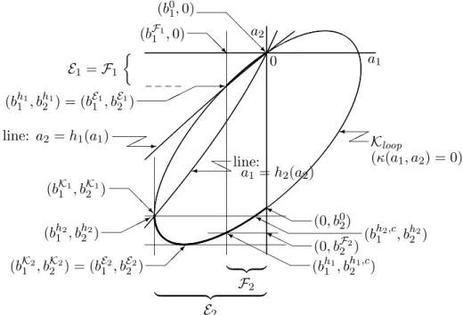
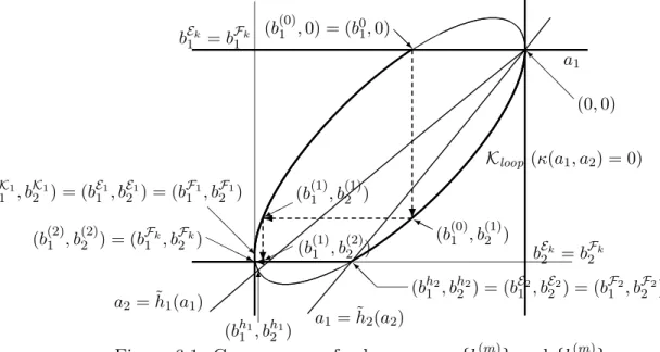
In order to describe our main theorem we introduce sets on the (a1, a2)-plane and num- bers related to them. First we note that, as will be shown in Lemma 7.1, the set
Kloop ={(a1, a2) : κ(a1, a2) = 0} (4.12) is a loop passing through the origin, i.e.κ(0,0) = 0 (see Figure 4.1 for an example). We let Ek ={(a1, a2)∈ Kloop : ak <0 and hk(ak)≤ak ≤0} and (4.13) bEkk = inf{ak : ∃ak such that (a1, a2)∈ Ek}. (4.14) Further we define
Fk = Ek∩ {(a1, a2) : ak ≥bEkk }
= {(a1, a2)∈ Kloop : ak<0 and max{hk(ak), bEkk } ≤ak ≤0}. (4.15) and let
ηk = exp{bFkk}, where bFkk = inf{ak : ∃ak such that (a1, a2)∈ Fk}. (4.16) As will be shown in Lemma 7.2, Ek and Fk are nonempty and the numbersbkEk, bFkk and ηk are all well defined. Our main theorem is stated as follows.
Theorem 4.1 ηk = exp{bFkk} is less than 1 and is greater than or equal to the decay rate η∗k of the marginal queue-length distribution {pk(n)} defined in (3.3), namely
ηk∗ ≤ηk <1. (4.17)
The proof of this theorem needs a long discussion using a series of lemmas. So we postpone it to Section 6.
Remark 4.1 (On the sets Ek and Fk) The set
Ek ={(a1, a2)∈ Kloop : ak<0 and hk(ak)< ak <0} (4.18) consists of points (a1, a2) satisfying the condition of Lemma 6.1 given in Section 6 together with constraintsak<0 and ak <0. Ek is almost the same as this set. However Ek becomes empty if hk(ak) ≡ 0 and hence if rkk = 0. To avoid this inconvenience and to make the exposition of the theorem general, Ek is slightly changed from Ek so that it is nonempty in any case. Fkis defined so that it provides the coordinate of the limit point of the converging
sequence of points given by (6.31) in Section 6. ♦
Remark 4.2 (An LST version) Theorem 4.1 can be restated in terms offk andgk directly.
For brevity of exposition, here we state the result only for the case λ2 > 0. If λ2 = 0, we have to change equations (4.19) and definitions (4.20) below slightly. From (3.16), (3.18) and (3.11), we have three equations for four variables x1, x2,y1 and y2 as
rk0fk(xk) +rkk+rkk fk(xk) fk(xk)
gk(−yk) = 1 for k= 1,2, and x1+x2−y1−y2 = 0.
(4.19)
We define positive numbers ˆxk and ηk as ˆ
xk = sup{xk : ∃(x1, x2, y1, y2) satisfying (4.19), xk ≥0, xk >0 and yk ≤0}, (4.20) ηk = inf{fk(xk) : ∃(x1, x2, y1, y2) satisfying (4.19), xk>0, xk ∈[0,xˆk] andyk ≤0}.
Then from relations in (4.7) we see ηk=ηk. ♦
Remark 4.3 (Corollaries on procedure) To calculatebF11 and bF22 in individual models, we shall write them more explicitly. We consider the curves and straight lines
κ(a1, a2) = 0 (the set Kloop), ak =hk(ak), ak = 0 and ak =bEkk (4.21) on the (a1, a2)-plane (see Figure 4.1 for an example). Properties of these curves and lines will be examined in Section 7. We start with introducing notations for some sets and coordinates of intersections of the curves and lines. We let
K={(a1, a2) : κ(a1, a2)≤0} and Kk ={(a1, a2)∈ K : ak ≤0}. (4.22) The set K is convex (Lemma 7.1) and its periphery is Kloop. For a given number b, the straight line ak =b either intersects with Kloop twice, is tangent to Kloop at a single point, or never meets Kloop. In the following discussions, for brevity of exposition, sometimes we say the line intersects withKloop at two points even when the line is tangent to the loop.
The straight line ak = 0 intersects with Kloop at two points, one of which is the origin (Lemma 7.1). Let b0k be the smaller k-th coordinate of the two intersections, namely
b01 = min{a1 : κ(a1,0) = 0} and b02 = min{a2 : κ(0, a2) = 0}. (4.23) The curve ak = hk(ak) intersects Kloop at two points, at the origin and at a point having negative coordinates (Lemma 7.1). Let (bh1k, bh2k) be the coordinates of the latter point, namely, for example, if k = 1,
bh11 ={unique negative root of equation κ(a1, h1(a1)) = 0 for a1} and bh21 =h1(bh11).
(4.24) The straight line ak =bhkk intersects Kloop at two points, one of which is (b1hk, bh2k). Let bhkk,c be the k-th coordinate of the other intersection. Namely, for example, if k = 1,
bh21,c = root other thanbh21 of equationκ(bh11, a2) = 0 for a2. (4.25) We let
bK(k k)= inf{ak : ∃ak such that (a1, a2)∈ K}, and bKkk = inf{ak : ∃ak such that (a1, a2)∈ Kk}.
(4.26)