A Robust Tracking with Low-Dimensional Target-Specific Feature Extraction

(1)

PAPER

A Robust Tracking with Low-Dimensional Target-Specific Feature Extraction

Chengcheng JIANG^†, Xinyu ZHU^†, Chao LI^†,Nonmembers,andGengsheng CHEN^†a),Member

SUMMARY Pre-trained CNNs on ImageNet have been widely used in object tracking for feature extraction. However, due to the domain mismatch between image classification and object tracking, the submergence of the target-specific features by noise largely decreases the expression ability of the convolutional features, resulting in an inefficient tracking. In this paper, we propose a robust tracking algorithm with low-dimensional target- specific feature extraction. First, a novel cascaded PCA module is proposed to have an explicit extraction of the low-dimensional target-specific features, which makes the new appearance model more effective and efficient.

Next, a fast particle filter process is raised to further accelerate the whole tracking pipeline by sharing convolutional computation with a ROI-Align layer. Moreover, a classification-score guided scheme is used to update the appearance model for adapting to target variations while at the same time avoiding the model drift that caused by the object occlusion. Exper- imental results on OTB100 and Temple Color128 show that, the proposed algorithm has achieved a superior performance among real-time trackers.

Besides, our algorithm is competitive with the state-of-the-art trackers in precision while runs at a real-time speed.

key words: object tracking, feature extraction, PCA, CNN, particle filter

1. Introduction

Given a target in a bounding box, object tracking is to lo- calize and identify this target in the following video frames.

In many of its applications, i.e. video surveillance, object tracking is heavily challenged by various disturbances, such as non-rigid object deformation, occlusion, and illumination variation. In tracking, a robust appearance model is highly required to give an explicit discrimination of the target and to provide with invariances to intra-class variations of the target.

In an appearance model, feature extraction plays a crit- ical role. Due to the limited ability in representing a target, traditional handcrafted features (i.e. Gabor wavelet[1], op- tical flow[2], HOG[3],[4], SIFT[5], Color Name[6], etc.) have gradually been substituted by convolutional features extracted by CNNs (Convolutional Neural Networks). Re- searches[7],[8]use a pre-trained VGG-Net[9]as the basic feature extractor, after which correlation filters (CFs) are applied to learn the appearance of the target. These new convolutional features have increased tracking precision over traditional features. However, their simple adoption of convolutional features neglects the domain mismatch between

Manuscript received January 31, 2019.

Manuscript revised April 1, 2019.

Manuscript publicized April 19, 2019.

†The authors are with State Key Lab of ASIC and System, Fudan University, Shanghai, 201203 China.

a) E-mail: [email protected] DOI: 10.1587/transinf.2019EDP7032

general object classification and specific target tracking. For depicting a specifc target, the raw convolutional features contain pretty much noise and redundancy (i.e. those features responsible for classifying objects of other categories).

Thereby the trained correlation filters could be highly overfit. Moreover, these noise and redundancy have brought about an extra cost in computation when optimizing these correlation filters, resulting in a low tracking eﬃciency.

To handle the problem of domain mismatch, some recent works[10],[11]propose to append a domain-specific network to the pre-trained CNN layers and train this network on the tracking sequences to classify the target from its background. Though achieving state-of-the-art performance in precision, since these domain-specific networks are usually complex with large amount of parameters, updating such networks online heavily slows down the tracking speed, making these works unable to achieve real-time tracking.

Other methods[12],[13]tend to insert a target-specific feature extraction module before using the pre-trained convolutional features for target-background classification. The FCNT method[12] uses a backpropagation-guided feature map selection to pick out the most relevant feature maps for tracking. In TRACA[13], several category-dependent auto- encoders are trained oﬄine to compress the feature maps during tracking. The explicit removal of noise and redundancy in these works leads to high-quality low-dimensional features so that a light-weight network can be applied and updated online in the appearance model to identify the target. Therefore, a better balance between the precision and eﬃciency can be reached in these tracking algorithms. How- ever, existing target-specific feature extraction methods only apply channel-wise compression of the convolutional features, without considering the spatial redundancy and the disturbance from background.

In this paper, we propose a robust tracking algorithm with low-dimensional target-specific feature extraction. A novel cascaded PCA[14] module is proposed which contains a target-independent channel-level PCA and an extra target-level PCA. Concretely, we first apply a channel-level PCA to coarsely compress the feature maps. Then we attend to the target exclusively by incorporating a second target- level PCA, which is applied to features of target samples and background samples to extract low-dimensional target- specific features. The obtained target-specific features are used to train a logistic regression (LR) model for target- background classification. To levarage the ability of tra- Copyright c2019 The Institute of Electronics, Information and Communication Engineers

(2)

ditional particle filter in modeling complicated state transitions and to ease the computational burden during particle evaluation, we propose a fast particle filter process that brings in a ROI-Align layer[15]to share the convolutional computation. Moreover, to counteract model drift caused by occlusion and resume tracking in the case of losing the target, we propose an adaptive scheme to update the LR model and to increase the robustness of the tracking.

The main contributions of this paper are as follows:

• We propose a novel cascaded PCA module to extract low-dimensional target-specific features, which achieve a better discrimination of the target and increase the computational eﬃciency as well.

• We propose a fast particle filter process by applying a ROI-Align layer in the evaluation of particles to achieve extra speed gain.

• We propose an adaptive updating scheme for the appearance model to increase the robustness against occlusion and model drift.

• Experimental results on OTB100 and Temple Color128 show that the proposed tracking algorithm has achieved a superior performance both in precision and in speed.

The rest of this paper is organized as follows: Sect. 2 reviews the related works. Section 3 introduces the proposed appearance model with target-specific feature extraction. In Sect. 4, we detail the whole tracking algorithm based on the new appearance model, the fast particle filter and the adaptive updating scheme. Extensive experiments and analyses are given in Sect. 5, followed by a conclusion in Sect. 6.

2. Related Work

2.1 Motion Model in a Tracking Algorithm

A tracking algorithm can generally have three main con- stituents: motion model, appearance model and updating scheme. Motion model predicts the candidate states (i.e.

location, scale and shape) of a target in a new frame. Ap- pearance model evaluates these candidates to identify the target. Updating scheme keeps the appearance model up to date against target variations.

In recent correlation filter based tracking algorithms[4],[7],[8], the motion model is reduced to a convolutional operation, where candidates for the next frame are obtained by circularly shifting the current target in its neighborhood. The main problem of the correlation filter is its boundary eﬀect. When a target undergoes a fast motion or a dramatic deformation, the boundary eﬀect that caused by the circularly shifting will result in poor candidates of the target. To the contrary, the Bayesian particle filter[16],[17]

propagates a continuous probability distribution of a target’s state along time, which means it can provide with a better proposal of the candidates even if the target is in a complex motion. Besides, diﬀerent from the correlation filters that only accept the linear/kernelized regression models[4], the particle filter has a better adaptability to various kinds of

appearance models (i.e. subspace learning[18], structured SVM[19], neural networks[11]).

2.2 Appearance Model Updating

As a target may undergo appearance variations caused by the quick changes of illumination, deformation and rotation, an online updating is a necessary to the appearance model.

Most trackers[7],[8] perform a blind update according to the current tracking result. There exist two problems with this blind updating strategy. Firstly, it brings about the risk of incurring model drift. When the target is occluded, a large portion of background information is blended in. If we update the appearance model with contaminated samples, it will gradually drift to characterize the background rather than the target. Moreover, a long duration of occlusion might lead to a complete appearance model corruption.

Secondly, as the tracking process is unsupervised and au- tonomous, samples used to update the appearance model are not reliable. In the case that the target is already lost due to the abrupt motion of the target, large deformation, motion blur or other disturbances, persistent updating using the wrong tracking results will aggravate this failure via positive feedback mechanism, making it unrecoverable. Some algorithms use an occlusion detection[13],[20]or a failure detection[21]to avoid the above harmful updating. In this paper, based on our observation of classification score, we propose an adaptive updating scheme to keep the appearance model more robust.

2.3 Principle Component Analysis

Principle component analysis, also known as the discrete Karhunen-Loeve transform, filters out the noise and cor- relations in the original signals to obtain the new low- dimensional uncorrelated signals. PCA is widely used in computer vision tasks, such as image compression, object detection[22], and CNN compression[23]. In object tracking, PCA is firstly adopted in generative tracking algorithms to learn a subspace for representing the target[18]. As these algorithms do not make use of the background information, they have inferior performance under complicated scenarios. Recently, several discriminative tracking algorithms[3],[6],[24]exploit PCA to perform feature dimen- sionality reduction. In CREST[24], before adopting pre- trained convolutional features for tracking, a PCA is used to compress the channels of conv4-3 features in VGG-16.

In this way, CREST not only relieves the overfitting caused by noise and redundancy, but also accelerates the tracking.

However, as pointed out in the DRT method[25], the un- expected high responses in the feature maps caused by the salient background tend to misguide the tracking process, and a simple channel compression of the convolutional features is not enough to counteract this kind of disturbance from the complicated background. In this paper, we take a way of explicitly extracting target-specific features to sup- press the disturbance from the background.

(3)

2.4 Tracking Based on Deep Learning

There are already many previous researches on using deep learning based algorithms in tracking. Among them, researches[7],[8],[25]use the way of equipping traditional correlation filters with pre-trained convolutional features to enhance the robustness under tough scenarios, which might bring about a sacrifice of tracking eﬃciency due to the problem of domain mismatch. This kind of domain mismatch can be well reduced by training a domain-specific CNN on the current sequence to perform reliable classification of the target and its background, representative methods including multi-domain network[11], fully convolutional network[12], and CNN ensemble via tree structure[26]. To avoid the expensive online updating of the afore-mentioned domain-specific CNN architectures, several works[27]–[30] reformulate the object tracking as a general similarity matching task, with an adoption of a two- stream Siamese network to extract deep representations for the template patch and search patch simultanously. Af- ter that, a contrasive loss layer[27], a cross correlation layer[28], a regression layer[29], or a region proposal network[30]can be utilized to fulfill the tracking task. After trained on the large-scale external video datasets, no online updating is required during tracking, which enables a real- time speed in these methods.

In addition, RNN (Recurrent Neural Network) architecture and reinforcement learning are also promising direc- tions for further improving the performance of deep trackers. For instance, the SANet tracker[31]employs RNN to improve the robustness to intra-class distractors while the ACT tracker[32]optimizes the candidate searching process by using the ‘Actor-Critic’ framework.

In this paper, inspired by the superior class- discriminative ability of deep CNNs, we generate high-level target-specific representations to counter the problem of domain mismatch and to increase the tracking eﬃciency.

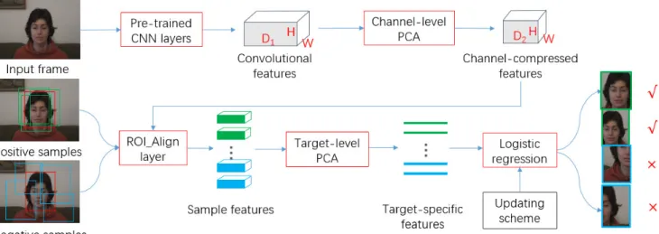
Fig. 1 Proposed appearance model with target-specific feature extraction.

3. Appearance Model with Target-Specific Feature Ex- traction

3.1 Proposed Appearance Model

Figure 1 shows the overall architecture of our appearance model. It mainly contains three parts: pre-trained CNN layers, two cascaded PCAs and a logistic regression (LR) model.

The pre-trained CNN layers are used to extract the convolutional features of the current frame, which are then processed by a channel-level PCA to obtain the channel- compressed features. Image samples (i.e. image patches) are randomly cropped around the target. These image samples and channel-compressed features are fed to a ROI- Align layer to get sample features. The target-level PCA is thereafter performed on these sample features to extract low-dimensional target-specific features. Finally, a logistic regression model takes the target-specific features as its inputs and calculates the classification scores of these samples. In addition, the updating scheme updates the LR model dynamically.

3.2 Channel-Level PCA

We extract the convolutional features of an image frame with a pre-trained VGG-16. However, the generated convolutional features are usually sparse with much redundancy due to the domain mismatch between image classification and object tracking. Thus, a channel-level PCA is intro- duced to compress the convolutional features.

PCA[14] is a linear transformation for dimensional- ity reduction with its objective function given in Eq. (1).

xi ∈ R^D¹ is the original feature vector, P^Txi ∈ R^D² is the compressed new feature vector (D₂ D₁), P is the or- thogonal projection matrix which has a closed-form solu- tion by using SVD (Singular Value Decomposition)[14].

(4)

Fig. 2 Scree plot of channel-level PCA forWomansequence.

The column vectors ofP, called principle components, are equal to the left singular vectors of the feature matrix X (X = (x1,x2, . . . ,xN)). Principle components construct a set of base vectors for the new feature space, where the re- covery error between{P^Txi}i^N=1and{xi}^N_i₌₁is minimized, as shown in Eq. (1). Each principle component is associated with a value denoting its percentage of explained variances (i.e. the importance of this principle component for reserv- ing the information).

P=arg min

P∈R^D^1×D2

1 N

i

xi−PP^Txi²₂

s.t.P(:,j)²₂=1,P(:,j)^TP(:,k)=0 whenjk (1)

In the channel-level PCA processing, we combine the convolutional features to form a feature matrix X with its dimension to beC×(W∗H), whereCis the original channel number of convolutional features (i.e. 256 in VGG-16 conv3-3), W and H are the width and height of a feature map. Throughout the PCA training, the number of remained principle components (i.e.D₂) depends on the percentage of variances we wish to reserve. Figure 2, takingWomanse- quence as an example, gives the scree plot of the percentage of explained variances (PEV) versus each principle component in a descending order. It can be seen that the PEV distributions are sparse, with most variances focused on only a few principle components. Since those principle components with small PEV values have little contribution to the characterization of the target, we can remove them from the convolutional features with negligible impacts to the whole processing quality. According to our cross validation and analysis in Sect. 5.4.1, an appropriate setup for achieving a good compression of channels is thatD2=128, with which we decrease the number of channels by 50% while having a negligible loss of the original information (roughly 10%).

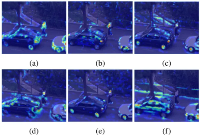
By compressing the channels, channel-level PCA filters out a portion of noise and redundancy in the convolutional features. However, there still exist other kinds of redundancy (i.e. disturbance) in the obtained channel- compressed features, which are resulted from the distractors in the background. Figure 3 shows an example of six compressed feature maps for theWomansequence. We can see

Fig. 3 Example feature maps of channel-compressed features. To better visualize the responses to the target-under-tracking (i.e. the woman) and its background, we blend each feature map with the original image by a ratio of 3 : 2.

that, these compressed feature maps have strong responses both to the patterns of concern (the woman in the image) and to other salient objects (the cars) in its background. The feature map in Fig. 3 (f) even presents no response to the target. Thus compressing the feature maps holistically is not enough for extracting target-specific features.

3.3 Target-Level PCA

A target-level PCA is thereafter designed and used to extract the target-specific features for a more eﬃcient discrimination of the target samples from its background. Let pi

be an image sample and{pi}Nbe an assembly of N samples, these image samples can be positive (S₊, indicating the “target”) and negative (S₋, indicating the “background”). Fig- ure 1 shows an example of the image samples with the green boxes indicating the positive samples and the blue boxes indicating the negative samples. A ROI-Align layer is used to obtain the features of these samples according to their geometric positions from the channel-compressed features.

These sample features are denoted as{ri}_i^N₌₁whererihas a fixed shape ofD₁ ×(7∗7). The target-level PCA is then trained on {vec(ri)}^N_i₌₁ with the same process as channel- level PCA does.

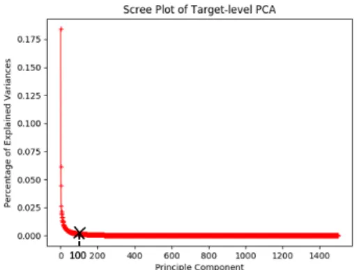
As shown in Fig. 4, for the target-level PCA, the PEV curve has an abrupt decrease at the point near the origin.

Compared with the channel-level PCA, there is a much smaller portion of principle components that make contribution to the total accumulated variances, which means a lot of noise and redundancy exist in the sample features. Accord- ing to our experiments, we find that an optimal tracking performance can be reached by retaining the top-ranking principle components that contain about 90% of the variances.

With this setup, we have the final target-specific featureti

(ti ∈R^D) to be with a typical dimension of 100. Compared with the original sample features, the target-specific features achieve a compression ratio of more than 50 (the dimension oftivsri). Therefore, the extraction of target-specific features not only gives a better characterization of the target,

(5)

Fig. 4 Scree plot of target-level PCA forWomansequence.

but also largely reduces the feature dimension. Both of these eﬀects allow for adopting a high-eﬃciency classifier to discriminate the target from its background during tracking.

3.4 Classifying Using Target-Specific Features

Using the target-specific features, a light-weight logistic regression model is able to be trained to classify the target samples and background samples. As shown in Eq. (2), the logistic regression modelφtakesti(target-specific feature) as its input and outputs a score si to indicate whether its corresponding image sample pi is the target under tracking or not, in the sense of probability (i.e.siis in the range of [0,1]). wLR is the model parameters trained on{ti, yi}N, whereyi =1 for a positive sample oryi =0 for a negative sample. In the design, we updatewLRonline according to the logistic loss and the regularization loss, as given in Eq. (3).

si=φ(ti|wLR)= 1

1+e⁻^w^T^LR^tⁱ (2)

loss=−1 N

N

i=1

yilogsi+(1−yi)log(1−si)+λwLR²₂ (3)

3.5 Data Pre-Processing and Augmentation

In PCA calculations, if a feature has a noticeably large value in its magnitude, it will dominate the optimization of the objective function even though its relative variance has a small value. This will prevent the PCA from learning other discriminative features. Thus, we need to normalize the feature matrix before performing the channel-level PCA and the target-level PCA.

In tracking, data deficiency is an inherent problem as the target is given only once in the first frame. We solve this problem by data augmentation. Specifically, the positive samples used to train our target-level PCA and the logistic regression model are augmented in the following methods:

(1) Sample the image patches around the target randomly if the IoU (Intersection over Union) with the target is higher than a threshold;

(2) Scale the target randomly within the range of [0.8,1.2];

(3) Rotate the target randomly within the range of [−10^◦,10^◦];

(4) Blur the target using a Gaussian filter with its kernel size of (5,5) and its variance randomly selected in the range of [0.8,1.2];

(5) Flip the target horizontally and sample image patches around the flipped target in the same method as (1).

This augmentation of positive samples increases the robustness of our appearance model as well.

4. A Robust Tracking Using Target-Specific Features With the appearance model to discriminate the target from its background, a fast particle filter process and an adaptive updating scheme are used for our robust tracking. When a new frame arrives, the particle filter predicts multiple candidate samples (so-called particles) according to the prior kinetics knowledge and rectifies the prediction based on the classification scores from the appearance model. The adaptive updating scheme is used to update the appearance model dynamically and reliably during tracking. Algorithm 1 gives our proposed tracking algorithm.

Algorithm 1Tracking with target-specific features

Input: Pre-trained VGG-16, initial target statep¹. Output: Estimated target statep^t_∗for each frame.

1: Propagate the first frame into VGG-16 and train channel-level PCA using conv3-3 features.

2: Collect positive samplesS¹₊and negative samplesS¹₋,{p¹_i, y¹_i}_N ← S¹₊∪S¹₋.

3: Train target-level PCA using{p¹_i, y¹_i}. 4: Train LR model{wLR}using{p¹_i, y¹_i}. 5: Initialize particles{q¹_i =p¹}_N_q. 6: repeat

7:

8: ifenough failures are observedthen

9: Re-detectp^t_∗, re-initialize particles{q_i^t=p^t_∗}_N_q. 10: Update training dataS^t_{+_,_−}and update LR model{wLR}. 11: Continue to process the next frame.

12: end if

13: Predict new particles{q^t_i}from distributionp(q^t_i|q^t−1_i ).

14: Calculate classification scores{s^t_i}as in Fig.1.

15: Update normalized particle weights{w^t_i}by Eq. 9.

16: Estimate target statep^t_∗by Eq. 10.

17: Resample particles{q^t_i}according to{w^t_i}. 18:

19: ifs^t_maxis higher thanThthen

20: Collect new positive samples K₊^t and negative samplesK₋^t aroundp^t_∗.

21: Update training dataS^t_{+_,_−}. 22: end if

23:

24: ifscore fluctuations are detectedthen 25: Update LR model{wLR}usingS^t_{+_,_−}. 26: end if

27: untilend of the sequence.

(6)

4.1 Fast Particle Filter Process

Particle filter recursively solves for the posterior distribution of the target states by using a finite set of weighted particles {q^t_i, w^t_i}. It has been widely applied to tracking due to its superior ability to keep high-confident candidate states of the target and to deal with complicated target motion.

In our tracking algorithm, a particle q^t_i is represented by a quadruple (x, y, α, β) where (x, y) denotes the center of the target and (α, β) denotes its size and aspect ratio. We assume that, in a short period of time, the target moves at a constant velocity with Gaussian noise. The state variations of scale and aspect ratio are also sampled from Gaussian distributions. Equation (4)∼(7) illustrate these four state transitions, whereσ²_x, σ²_y, σ²_α, σ²_β are variances of the Gaus- sian processes that set to be 0.2∗( width of the target )², 0.2∗( height of the target)², 0.01, 0.01 respectively during tracking. Thus in Eq. (8), the state transition ofqi is the combination of these four individual transitions.

Equation (9) calculates the normalized weight of each particle based on the classification scores^t_iwhich is obtained in the appearance model. Note that this evaluation of particles is especially computationally expensive and has be- come a bottleneck of the whole tracking pipeline.

To solve this problem, in this paper, instead of propagating each particle into the pre-trained CNN layers and the subsequent channel-level PCA, we directly compute the sample features of these particles from the channel- compressed features of the image frame by using a ROI- Align layer, as shown in Fig. 1. Then these sample features are fed to the logistic regression to calculate the classification scores. In this way, we share the convolutional computation and channel-level PCA computation among particles, which largely accelerates the evaluation of particles.

After the evaluation of particles, we can finally estimate the target statep^t_∗by weighing the states of those particles whose weight is higher than a thresholdTs∗w^t_maxas shown in Eq. (10), where1(·) is the indication function used to sift out these high-weight particles andZ is the sum of their weights.

The entire procedure of the fast particle filter is pre- sented inAlgorithm1 line13∼line17.

p(x_i^t|x^t_i⁻¹)∼N(2∗x_i^t⁻¹−x^t_i⁻², σ²_x) (4)

p(y_i^t|y^t_i⁻¹)∼N(2∗y_i^t⁻¹−y^t_i⁻², σ²_y) (5)

p(α^t_i|α^t_i⁻¹)=p( α^t_i

α^t_i⁻¹)∼N(1, σ²_α) (6) p(β^t_i|β^t_i⁻¹)=p( β^t_i

β^t_i⁻¹)∼N(1, σ²_β) (7) p(q_i^t|q^t_i⁻¹)=p(x^ti|x_i^t⁻¹)∗p(y^t_i|y^t_i⁻¹)

∗p(α^t_i|α^t_i⁻¹)∗p(β^t_i|β^t_i⁻¹) (8)

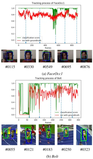
Fig. 5 The classification scores ofFaceOcc1sequence (a) andBoltse- quence (b). In the bottom are the predicted target (green box) and its ground truth (blue box) drawn qualitatively on the frames to facilitate our analysis.

w^t_i= s^t_i

js^t_j (9)

p^t_∗= 1 Z

N_q

i=1

1(w^ti>Ts∗w^t_max)∗w^t_i∗q^t_i (10)

4.2 Adaptive Updating Scheme

The updating scheme of the appearance model has a large influence on the robustness of tracking. In this paper, we propose a classification-score guided updating scheme.

The classification scores of the particles can present different patterns under different scenarios, especially when the target is under occlusion, deformation or disappearance (here the term ‘disappearance’ means the tracker suffers a sudden lost of the target and needs a re-detection). Figure 5 shows the classification scores during tracking ofFaceOcc1 and Bolt, where the green curve depicts the classification score of the predicted target, the red curve depicts the IoU score between the predicted target and its ground truth, and

(7)

the qualitative results are given in the bottom. InFaceOcc1, the classification score decreases consistently as occlusion degree increases (frames #0115, #0330, #0549, #0695 and

#0876). InBolt, the classification score fluctuates when the target undergoes large pose variations (frames #0121, #0250 and #0323). When we have lost the target, the classification score remains at a low value (frames #0008∼#0055) until the target is re-detected in the frame #0056.

Therefore, using the classification scores to be aware of diﬀerent scenarios, diﬀerent actions are applied accord- ingly:

(1) to alleviate model drift caused by occluded samples, we collect new training samples only when the classification score is higher than a threshold Th (i.e. 0.7).

Then, we update the training dataS^t_{+_,_−} in a memory- friendly way: old positive samples and negative samples are randomly replaced by new ones that collected at the current frame. In this way, the size of the training data remains unchanged, which can save the memory cost during the proceeding of tracking;

(2) when the classification score fluctuates in accordance with target variations, we update logistic regression model using the training dataS^t_{+_,_−};

(3) when the classification score is lower than a threshold Tl (i.e. 0.5), we record one failure. In the case that a certain number of successive failures are observed, we trigger a re-detection process (i.e. search for the target in the whole frame) to resume the tracking of the lost target.

Algorithm1 (line 8, 19, 24) gives the details of our adaptive scheme. By this special design of the updating scheme, we are able to increase the robustness of our tracking algorithm, especially when the target is occluded.

5. Experiments and Analyses

5.1 Experimental Setup

We implement and test our tracking algorithm with python interface on Caﬀe^†, using an Nvidia GTX 1080ti GPU and an Intel i7-7700K CPU. The first seven convolutional layers (conv1-1∼conv3-3) of VGG-16, pre-trained on Ima- geNet[33], are used as our convolutional feature extractor.

The mean-subtracted image frames of the sequences are fed to these convolutional layers for the extraction of features.

We assign a positive label to an image sample if its IoU score with the ground truth is higher than 0.8 and a negative label if its IoU score is lower than 0.3. In order to balance between computational cost and precision, we set the size of our training dataS^t_{+_,_−}to be 1500, with a positive-negative ratio (#{S₊} : #{S₋}) of 1 : 2. In the channel-level PCA, we retain the 128 top-ranking principle components. In the target-level PCA, in consideration of the diﬀerence existed in various targets, we adaptively select the number of retained principle components to keep 90% of the variances.

†Oﬃcial website: http://caﬀe.berkeleyvision.org

After training channel-level PCA and target-level PCA in the first frame, their projection matrices are fixed in the subsequent frames. The regularization strengthλin Eq. (3) is set to be 0.005. Since only recent negative samples are relevant to the current tracking, we set #{K₊} to be 100 and set #{K₋}to be 400. These new samples (K_{+,−}) are collected every three high-score frames. We keep 100 particles and perform multinomial resampling each frame to keep the particle active. The threshold valueTsin Eq. (10) is set to be 0.5. Throughout the tests, all the above-mentioned settings are fixed unless otherwise specified.

5.2 Evaluation Methods

We evaluate our tracking algorithm on two challenging benchmarks, OTB100[34]and Temple Color128[35](TC- 128). OTB100^††contains 98 sequences each tagged with 11 attributes, while TC-128^††† has 128 color sequences with ground truth and challenging factor annotations. We perform one-pass evaluations (OPE) for our proposed tracking algorithm on both OTB100 and TC-128, generating the precision plots and success plots respectively on all the sequences. The precision plot illustrates the percentage of the frames that have their location distance between the predicted target and the ground truth less than a threshold. All the trackers are ranked according to their precision scores at the threshold of 20 pixels. Whereas the success plot illustrates the percentage of the frames that have their IoU scores between the predicted target and the ground truth higher than a threshold. All the trackers are ranked according to their AUC (Area Under Curve) scores.

5.3 Analyzation of Target-Specific Features

To verify whether the extracted target-specific features are eﬀective for the task of target-background classification or not, we embed the samples represented by the target-specific features in a two-dimensional space using t-SNE[36] to clearly visualize the distributions of these samples. The t-SNE method models the similar samples in the original target-specific feature space by adjacent points and models those dissimilar ones by distant points. Figure 6 shows our experimental results of the Woman sequence, where Sample-A are negative samples, Sample-B are positive samples generated via shifting, rotating, scaling and blurring the target (method (1)∼(4) in Sect. 3.5), Sample-C are positive samples generated around the horizontal-flipped target (method (5) in Sect. 3.5).

From Fig. 6 we can see that:

(1) in the new feature space generated by our cascaded PCAs, positive samples are well separated from negative samples. This proves that although we do not

††Dataset website: http://cvlab.hanyang.ac.kr/ tracker benchmark/datasets.html

†††Dataset website: http://www.dabi.temple.edu/˜hbling/data/

TColor-128/TColor-128.html

(8)

Fig. 6 Targer-specific features embedded in a two-dimensional space using t-SNE.

perform supervised fine-tune of VGG-16 on the video sequences, our extracted target-specific features by cascaded PCAs are clearly discriminative to represent the target which largely helps to simplify the task of target- background classification;

(2) the positive samples obtained around the horizontal- flipped target (Sample-C) are separated from other positive samples (Sample-B), which indicates that the ro- tational invariance of the target-specific features is reliable only when the rotation angle is small.

5.4 Analyzation of Key Parameters

The number of retained principle components in the channel-level PCA and the number of particles are two crit- ical parameters in our algorithm. To explore their impacts on the overall performance, extensive experiments are conducted on OTB100. To make the results more reliable, we repeat the experiment on each setting six times and average the results to produce our final estimation.

5.4.1 Number of Retained Principle Components in Channel-Level PCA

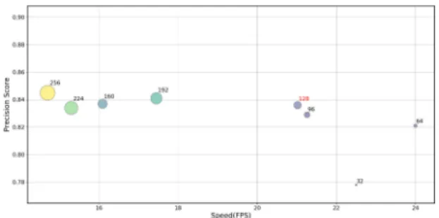
To discover how the number of retained principle components in channel-level PCA affects the tracking, we conduct an extensive test by applying eight different values: 32, 64, 96, 128, 160, 192, 224 and 256, with the results illustrated in Fig. 7. It can be seen that although the highest precision can be reached when we retain all the 256 principle components, it does not bring us much difference in tracking precision to have the retained number of principle components to be between 128 and 256. This well confirms that the pre-trained convolutional features contain pretty much noise and redundancy when directly applied in tracking and a channel compression is highly required for increasing the tracking efficiency. Besides, when we decrease the retained number to 32, there appears an obvious drop of the tracking precision, which tells us that an excessive removal of those principle components with non-negligible PEV values will bring about a significant loss of the capability in characteriz- ing the target and thereby will lead to an unaffordable impact to the tracking precision. Generally, we can find out that the

Fig. 7 Precision score and speed of our tracking algorithm on OTB100 when retaining diﬀerent number of principle components in channel-level PCA.

Fig. 8 The performance of our tracking algorithm on OTB100 when different number of particles is used.

retained number of principle components in channel-level PCA does have a negative correlation relationship with the overall tracking speed but not that strictly, which can be attributed to the reason that other factors such as target-level PCA manipulations and the frequency of adaptive online updating will also aﬀect the tracking speed. Therefore, in order to have an optimal balance between the precision and the speed, we select to retain 128 principle components in our channel-level PCA.

5.4.2 Number of Particles

To investigate how the number of particles aﬀects the tracking, another extensive test is conducted by varying the number of particles from 50 to 500, with a step of 50. With the results shown in Fig. 8, we can see that although the processing speed in FPS (Frames Per Second) decreases as the number of particles increases, the decreasing rate is much slower than linear. This can be attributed to our using of the ROI-Align layer to share the convolutional computation among particles. Besides, the tracking precision (reflected by precision score and AUC score) does not get strictly im- proved when we further increase the number of particles, especially in the range from 150 to 250. Therefore, choos- ing the number of particles to be 100 is an optimal balance to obtain a favorable precision and a real-time processing speed.

5.5 Experimental Results on OTB100

We test and evaluate our tracking algorithm on OTB100 and compare our results with several high-performance trackers.

(9)

5.5.1 Comparison with Real-Time Trackers

We first compare our tracking algorithm with several real-time trackers, including BACF[37], MEEM[38], KCF HOG[4], DSST[3] which use handcrafted features for target representation and TRACA[13], SiamFC[28], CFNet[39]which are based on deep convolutional features.

From the experimental results shown in Fig. 9 (a), our tracking algorithm (denoted as “Ours”) surpasses all these seven trackers in precision. Another advanced real-time tracker PTAV[41]unifies a traditional feature based tracker and a CNN based verifier in a single framework to leverage both the fast speed of traditional feature and the strong discrimi-

Fig. 9 Precision plot (a) and success plot (b) on OTB100 compared with other real-time trackers.

Fig. 10 Attribute-based evaluations on OTB100.

nation ability of CNN. Compared to PTAV, our precision is just slightly inferior but still comparable.

From the success plot in Fig. 9 (b) we can see that, in comparison with these eight trackers, our algorithm has achieved a favorable performance in the case when a loose overlap threshold (<0.3) is used. To make full use of our low-dimensional target-specific features in tracking and to reduce the model complexity, we adopt a logistic regression model to perform a brute binary classification of image samples rather than regressing a Gaussian function according to the spatial distance between the sample and the ground truth.

The used label assignment scheme with a fixed threshold on IoU score (0.3 for negative, 0.8 for positive) may bring about a slight decrease in the middle region of the success plot, which is acceptable as a trade-oﬀfor processing speed.

The attribute-based evaluations are performed as well.

As shown in Fig. 10, our algorithm has a robust and stable performance under diﬀerent complicated scenarios. Faced with the background clutter (Fig. 10 (b)), by performing a target-level PCA, we have a better suppression of the dis- turbing objects in the background. Notably, benefited from the classification-score guided updating scheme, our algorithm has exhibited a stronger capability in handling occlusion (Fig. 10 (i)) and out-of-view (Fig. 10 (g)). Besides, when the target has a fast motion (Fig. 10 (j)), owing to the boundary eﬀect, those algorithms based on correlation fil-

(10)

Fig. 11 Tracking results of 9 real-time trackers on 6 challenging sequences from the OTB100 benchmark (from left to right and top to down areLemming,Liquor,Girl2,Jumping,Panda,Tiger1).

ters (i.e. TRACA, DSST, KCF) have an obvious decrease in precision. In BACF, a background-aware filter design and an expanded search region are applied to reduce the boundary eﬀect, which enables BACF to work well under fast motion. While in our algorithm, the use of particle filter in our motion model helps to provide with a better proposal of the candidates even if the target is in a complex motion. As a result, we also have a favorable track of fast moving targets.

In summary, by using the target-specific features, our tracking algorithm has achieved an outstanding performance in comparison with the above real-time trackers especially under background clutter. Moreover, benefitted from our combinational use of the adaptive updating scheme and the motion model with particle filter, our tracking algorithm has strong robustness against occlusion and fast motion. Fig- ure 11 gives the qualitative results under diﬀerent complicated scenarios.

5.5.2 Comparison with State-of-the-Art Trackers

In addition to the above real-time trackers, we also compare our tracking algorithm with four state-of-the-art works (DLSSVM[40], CREST[24], HCFT[7] and MDNet[11]) in terms of the tracking precision and eﬃciency. To make fair comparison, we conduct the experiments under the same hardware platform. The obtained results of the precision score and the FPS are given in Table 1.

Instead of extracting the traditional Lab color features to represent the target followed by a strong dual linear structured SVM as in DLSSVM, we use the target-specific features to give a better description of the target and a light- weight logistic regression to reduce the online updating burden. As shown in Table 1, our approach surpasses DLSSVM by a large margin of 6.8% in precision while runs 2x faster.

The same as our algorithm, other three trackers are also based on pre-trained convolutional features. HCFT trains three separate correlation filters on multi-scale convolutional features of VGG-16 to leverage the hierarchical attribute of CNN. But it does not have an appropriate

Table 1 Performance and eﬃciency comparison with state-of-the-art trackers on OTB100.

Tracker Precision score@20 FPS¹

CREST 0.837 2

HCFT 0.837 3

MDNet-BB-HM 0.816 2

DLSSVM 0.767 10

Ours 0.835 21

1To estimate the FPS of these trackers, we run them on the same hardware platform as denoted in Sect. 5.1. The long video sequence Car24 with 3059 frames is used as the benchmark.

processing of noise and redundancy in the original convolutional features. CREST reformulates the correlation filter to a diﬀerentiable convolutional layer, where the kernel size of this convolutional layer equals to the size of the target. By this way, the three major components (feature extraction, response map generation and model updating) of this tracker are well integrated into a unified network. However, optimizing this large-size convolutional kernel by SGD (Stochastic Gradient Decrease) is very expensive in both memory and computational cost. MDNet appends three fully connected layers (FCs) to the conv3-3 layer. The first two FCs learn target-specific features (in dimension of 512) and the third FC, which is equivalent to our logistic regression model, classifies the target samples and the background samples. MDNet learns target-specific features by performing a supervised training on both the ad- ditional video datasets and the sequences under tracking, while our cascaded PCAs require only two SVD operations to fulfill the same task which is more eﬃcient and favorable in performance. In Table 1, MDNet-BB-HM is a version of MDNet without bounding box regression and hard negative mining, which we bring in for an exclusive comparison of the target-specific feature extraction. The experimental results show that, compared with these three works, our tracking algorithm can achieve a competitive or even better performance in precision and run several times faster in speed.

(11)

Fig. 12 Precision plot (a) and success plot (b) on TC-128 compared with 7 state-of-the-art trackers.

Fig. 13 Evaluation results ofOurs,Ours-channel,Ours-conv4andOurs- svmon OTB100.

5.6 Experimental Results on TC-128

On the more challenging TC-128 benchmark, we compare our tracking algorithm with 7 trackers including PTAV[41], BACF[37], MEEM[38], Struck[19] and KCF[4] which perform high-accuracy real-time tracking, as well as MCPF[42]and DeepSRDCF[8]which achieve state-of-the- art tracking performance. The results are shown in Fig. 12.

In terms of precision score (Fig. 12 (a)), we have a clearly better performance than all the five real-time trackers. Compared with MCPF, although we have an inferior performance, it should be noted that our approach has a great advantage in eﬃciency (21 FPS vs 1 FPS). In the success plot (Fig. 12 (b)), our algorithm outperforms most of the above trackers. Compared with the top performance tracker PTAV, there is only a minor margin of 0.22%. Our competitive results on TC-128 benchmark prove again that our proposed algotithm is both robust and eﬃcient.

5.7 Ablation Study

Ablation studies are conducted to investigate the contribution of diﬀerent parts in our appearance model. Ours- conv4is an implementation of the tracking algorithm using a deeper conv4 layer instead of a conv3 as the convolutional feature extractor. Ours-channelis an implementation without the channel-level PCA,Ours-targetis an implementation without the target-level PCA andOurs-svmuses SVM instead of logistic regression as the classification model in Fig. 1. The results on OTB100 are given in Fig. 13.

When removing the target-level PCA, the trained logistic regression model is highly overfit due to the large amount

of model parameters and the limited training samples. As a result,Ours-targetis vulnerable to target variations and only performs well on those easy sequences, such asBoy,Fish, Football1,Man, andCarDark. So we do not have its re- sult included in Fig. 13 for comparison. This finding proves that our favorable performance is largely benefitted from the target-level PCA.

When using a deeper conv4 layer in our appearance model, the precision score drops by 3.2 points as shown in Fig. 13 (a). This seems to be opposite to the well-accepted knowledge in image classification that using deeper CNNs has better performance than shallow CNNs. We attribute this to the loss of spatial resolution in deeper convolutional layers. In tracking, the features are supposed to be not only discriminative, but also having high spatial resolution which attenuates inevitably when going deeper in a CNN. Features from conv3 reach a good balance of the both.

Besides,Ours-channelperforms worse thanOurs. The channel-level PCA helps to filter out a portion of noise features and helps to alleviate the computational burden of the target-level PCA, but in our entire appearance model it makes less contribution to the performance improvement than the target-level PCA.

The performance gap between OursandOurs-svmis narrow both in precision plot (Fig. 13 (a)) and success plot (Fig. 13 (b)), which proves that our extracted target-specific features are the main contributors for good tracking performance and match well with various classification models. However, as the intrinsic probability output of logistic regression is easier to integrate into the framework of Bayesian particle filter and the training of logistic regression is more eﬃcient than SVM, we finally adopt logistic regression as our classification model.

6. Conclusions

In this paper, we propose a robust tracking algorithm with low-dimensional target-specific feature extraction. We design a novel cascaded PCA module to extract low- dimensional target-specific features from the pre-trained CNN for real-time tracking. Our use of the target-specific features in the newly proposed appearance model has been proved to have a favorable discrimination of the target- under-tracking and be of highly computational eﬃciency.

We combine this appearance model with our proposed fast particle filter to solve for the posterior distribution of the target states. Finally, an adaptive updating scheme is applied to enhance the robustness against occlusion. Our experimental results on OTB100 and TC-128 show that the proposed tracking algorithm has achieved an outstanding performance both in precision and in processing speed.

References

[1] M. Li, Z. Zhang, K. Huang, and T. Tan, “Robust visual tracking based on simplified biologically inspired features,” International Conference on Image Processing, pp.4113–4116, 2009.

[2] Y. Wu and J. Fan, “Contextual flow,” IEEE Conference on Computer

(12)

Vision and Pattern Recognition, pp.33–40, 2009.

[3] M. Danelljan, G. H¨ager, F.S. Khan, and M. Felsberg, “Discrimina- tive scale space tracking,” IEEE Transactions on Pattern Analysis and Machine Intelligence, vol.39, no.8, pp.1561–1575, Aug. 2017.

[4] J.F. Henriques, R. Caseiro, P. Martins, and J. Batista, “High- speed tracking with kernelized correlation filters,” IEEE Transac- tions on Pattern Analysis and Machine Intelligence, vol.37, no.3, pp.583–596, March 2015.

[5] H. Zhou, Y. Yuan, and C. Shi, “Object tracking using sift features and mean shift,” Computer Vision and Image Understanding, vol.113, no.3, pp.345–352, 2009.

[6] M. Danelljan, F.S. Khan, M. Felsberg, and J.v.d. Weijer, “Adaptive color attributes for real-time visual tracking,” IEEE Conference on Computer Vision and Pattern Recognition, pp.1090–1097, 2014.

[7] C. Ma, J.-B. Huang, X. Yang, and M.-H. Yang, “Hierarchical convolutional features for visual tracking,” IEEE International Conference on Computer Vision, pp.3074–3082, 2015.

[8] M. Danelljan, G. H¨ager, F.S. Khan, and M. Felsberg, “Convolutional features for correlation filter based visual tracking,” IEEE Inter- national Conference on Computer Vision Workshops, pp.621–629, 2015.

[9] K. Simonyan and A. Zisserman, “Very deep convolutional networks for large-scale image recognition,” arXiv:1409.1556.

[10] Z. Teng, J. Xing, Q. Wang, C. Lang, S. Feng, and Y. Jin, “Robust object tracking based on temporal and spatial deep networks,” IEEE International Conference on Computer Vision, pp.1153–1162, 2017.

[11] H. Nam and B. Han, “Learning multi-domain convolutional neural networks for visual tracking,” IEEE Conference on Computer Vision and Pattern Recognition, pp.4293–4302, 2016.

[12] L. Wang, W. Ouyang, X. Wang, and H. Lu, “Visual tracking with fully convolutional networks,” IEEE International Conference on Computer Vision, pp.3119–3127, 2015.

[13] J. Choi, H.J. Chang, T. Fischer, S. Yun, K. Lee, J. Jeong, Y. Demiris, and J.Y. Choi, “Context-aware deep feature compression for high- speed visual tracking,” IEEE Conference on Computer Vision and Pattern Recognition, pp.479–488, 2018.

[14] E. Alpaydin, Introduction to Machine Learning, 3rd ed., ch. Dimen- sionality Reduction, pp.120–127, The MIT Press, 2014.

[15] K. He, G. Gkioxari, P. Doll´ar, and R. Girshick, “Mask r-cnn,” IEEE International Conference on Computer Vision, pp.2980–2988, 2017.

[16] M.S. Arulampalam, S. Maskell, N. Gordon, and T. Clapp, “A tu- torial on particle filters for online nonlinear/non-gaussian bayesian tracking,” IEEE Transactions on Signal Processing, vol.50, no.2, pp.174–188, Feb. 2002.

[17] Y. Li, H. Ai, T. Yamashita, S. Lao, and M. Kawade, “Tracking in low frame rate video: A cascade particle filter with discriminative ob- servers of diﬀerent life spans,” IEEE Transactions on Pattern Anal- ysis and Machine Intelligence, vol.30, no.10, pp.1728–1740, Oct.

2008.

[18] D.A. Ross, J. Lim, R.-S. Lin, and M.-H. Yang, “Incremental learning for robust visual tracking,” International Journal of Computer Vision, vol.77, no.1-3, pp.125–141, 2008.

[19] S. Hare, S. Golodetz, A. Saﬀari, V. Vineet, M.-M. Cheng, S.L.

Hicks, and P.H.S. Torr, “Struck: Structured output tracking with kernels,” IEEE Transactions on Pattern Analysis and Machine In- telligence, vol.38, no.10, pp.2096–2109, Oct. 2016.

[20] Q. Chu, W. Ouyang, H. Li, X. Wang, B. Liu, and N. Yu, “On- line multi-object tracking using cnn-based single object tracker with spatial-temporal attention mechanism,” IEEE International Confer- ence on Computer Vision, pp.4846–4855, 2017.

[21] M. Wang, Y. Liu, and Z. Huang, “Large margin object tracking with circulant feature maps,” IEEE Conference on Computer Vision and Pattern Recognition, pp.4800–4808, 2017.

[22] P.F. Felzenszwalb, R.B. Girshick, D. McAllester, and D. Ramanan,

“Object detection with discriminatively trained part-based models,”

IEEE Transactions on Pattern Analysis and Machine Intelligence, vol.32, no.9, pp.1627–1645, Sept. 2010.

[23] S. Lin, R. Ji, X. Guo, and X. Li, “Towards convolutional neural networks compression via global error reconstruction,” International Joint Conference on Artificial Intelligence, pp.1753–1759, 2016.

[24] Y. Song, C. Ma, L. Gong, J. Zhang, R.W.H. Lau, and M.-H. Yang,

“Crest: Convolutional residual learning for visual tracking,” IEEE International Conference on Computer Vision, pp.2574–2583, 2017.

[25] C. Sun, D. Wang, H. Lu, and M.-H. Yang, “Correlation tracking via joint discrimination and reliability learning,” IEEE Conference on Computer Vision and Pattern Recognition, pp.489–497, 2018.

[26] H. Nam, M. Baek, and B. Han, “Modeling and propagating cnns in a tree structure for visual tracking,” arXiv:1608.07242.

[27] R. Tao, E. Gavves, and A.W.M. Smeulders, “Siamese instance search for tracking,” IEEE Conference on Computer Vision and Pat- tern Recognition, pp.1420–1429, 2016.

[28] L. Bertinetto, J. Valmadre, J.F. Henriques, A. Vedaldi, and P.H.S.

Torr, “Fully-convolutional siamese networks for object tracking,”

European Conference on Computer Vision, vol.9914, pp.850–865, 2016.

[29] D. Held, S. Thrun, and S. Savarese, “Learning to track at 100 fps with regression networks,” European Conference on Computer Vi- sion, vol.9905, pp.749–765, 2016.

[30] B. Li, J. Yan, W. Wu, Z. Zhu, and X. Hu, “High performance visual tracking with siamese region proposal network,” IEEE Conference on Computer Vision and Pattern Recognition, pp.8971–8980, 2018.

[31] H. Fan and H. Ling, “Sanet:structure-aware network for visual tracking,” IEEE Conference on Computer Vision and Pattern Recognition Workshops, pp.2217–2224, 2017.

[32] B. Chen, D. Wang, P. Li, S. Wang, and H. Lu, “Real-time

‘actor-critic’ tracking,” European Conference on Computer Vision, vol.11211, pp.328–345, 2018.

[33] J. Deng, W. Dong, R. Socher, L.-J. Li, K. Li, and F.F. Li, “Ima- genet: A large-scale hierarchical image database,” IEEE Conference on Computer Vision and Pattern Recognition, pp.248–255, 2009.

[34] Y. Wu, J. Lim, and M.-H. Yang, “Object tracking benchmark,” IEEE Transactions on Pattern Analysis and Machine Intelligence, vol.37, no.9, pp.1834–1848, Sept. 2015.

[35] P. Liang, E. Blasch, and H. Ling, “Encoding color information for visual tracking: Algorithms and benchmark,” IEEE transactions on image processing, vol.24, no.12, pp.5630–5644, Dec. 2015.

[36] L. van der Maaten and G. Hinton, “Visualizing data using t-sne,”

Journal of Machine Learning Research, vol.9, pp.2579–2605, 2008.

[37] H.K. Galoogahi, A. Fagg, and S. Lucey, “Learning background-aware correlation filters for visual tracking,” IEEE Interna- tional Conference on Computer Vision, pp.1144–1152, 2017.

[38] J. Zhang, S. Ma, and S. Sclaroﬀ, “Meem: Robust tracking via multiple experts using entropy minimization,” European Conference on Computer Vision, vol.8694, pp.188–201, 2014.

[39] J. Valmadre, L. Bertinetto, J. Henriques, A. Vedaldi, and P.H.S.

Torr, “End-to-end representation learning for correlation filter based tracking,” IEEE Conference on Computer Vision and Pattern Recog- nition, pp.5000–5008, 2017.

[40] J. Ning, J. Yang, S. Jiang, L. Zhang, and M.-H. Yang, “Object tracking via dual linear structured svm and explicit feature map,”

IEEE Conference on Computer Vision and Pattern Recognition, pp.4266–4274, 2016.

[41] H. Fan and H. Ling, “Parallel tracking and verifying: A framework for real-time and high accuracy visual tracking,” IEEE International Conference on Computer Vision, pp.5487–5495, 2017.

[42] T. Zhang, C. Xu, and M.-H. Yang, “Learning Multi-task correlation particle filters for visual tracking,” IEEE Transactions on Pat- tern Analysis and Machine Intelligence, vol.41, no.2, pp.365–378, Feb 2019.