Vu Tuan Khai
1. Introduction
Understanding the dynamics of the current account is one of the main themes in interna-tional macroeconomics. Understanding the dynamics of the current account becomes even more important in the world today given the problem of global imbalances with the U.S. running a large and persistent current account deficit on the one hand, and a number of other countries, including Asian countries, and China in particular, running large and per-sistent surpluses on the other hand. This problem has been attracting much attention from both economists and policy makers. What are the main determinants of the dynamics of the current account? What role can macroeconomic policy play in correcting the current account imbalances? These questions are of great interest and need to be answered. In the literature, many studies adopt the structural vector auto-regression (VAR) approach to analyze the current account. One problem of them is that they often rely on ad hoc as-sumptions to go from the reduced form to a structural interpretation with the VAR. For example, to identify shocks that affect the current account from data, many studies use the Blanchard-Quah long run restriction or the Cholesky decomposition, for which the reason-ing is informal rather than bereason-ing based on an explicit theory with a firm micro-foundation although the latter is unquestionably desirable.
The objective of this paper is to investigate the dynamics of the current account in a theo-retical model. The framework I utilize is a New Keynesian dynamic stochastic general equilibrium (DSGE) model of a small open economy, which has a firm micro-foundation and is flexible enough to incorporate many important factors relevant to the problem I wish to study. With the constructed model at hand, I calibrate it to the data of Thailand to make the analysis realistic, and then use it to study the effects of various structural shocks on the economy as a whole and the current account in particular. The focus of the present paper is the dynamics of the current account in the short run. The paper serves as a first step towards a study that I plan to conduct to analyze the determinants that govern the dy-namics of the current account of Asian countries.
Current Account Dynamics in a New Keynesian
Small Open Economy Model
The rest of paper is organized as follows. Section 2 describes the model. Section 3 ana-lyzes the affects of various types of structural shocks. Section 4 concludes.
2. The Model
In this section we build a New Keynesian DSGE model of a small open economy, which is rich enough to capture the dynamics of the current account. The model is a variant of the one developed in Shioji, Vu and Takeuchi (2009) with the main difference being that the production structure of the economy is revised to be more suitable for the reality of Asia that I keep in mind. There are four types of firms in this economy, and hereafter we shall call them (and the sector to which they belong) N, I, M, and X firms. N firms produce a ho-mogenous final good by combining domestic and imported intermediate goods. I firms are domestic intermediate goods producers, and M firms are importers of foreign intermediate goods. X firms are exporters which produce goods and sell exclusively to the foreign mar-ket. In the short run, firms in sectors I, M, and X might face sticky prices. Price stickiness is introduced in the form of the Rotemberg-type quadratic price adjustment costs, and is meant to give a role for monetary policy in affecting the real side of the economy. More-over, price stickiness in sectors M and X is meant to capture the possibly incomplete and slow pass through of the nominal exchange rate to import and export prices, which will be important for the dynamics of the current account.
Households
There are many households in the economy who lives infinitely and are distributed in the range [0,1]. Here the population is normalized to be unity. Households work, consume goods, pay taxes to the government, and save in the form of holding money and bonds using their wage income and dividends received from domestic firms which they own. Households derive utility from consuming goods and holding money, and disutility from working. Thus money is introduced into the model in the form of money in the utility function, in which we implicitly assume that money facilitates people’s transactions and thus enhances their utility. The expected life-time utility of a representative household is
, (1)
where Et denotes expectation at time t, is the subjective discount factor, and are consumption, work hours, and real money holdings, respectively. The period utility is specified as
, (2) where are parameters. Here, is the inverse of the intertemporal elasticity of substitution, is the inverse of Frisch labor supply elasticity, and are the weights placed on disutility from labor and utility from money holdings, respectively. The budget constraint of the household is
. (3) where M, B, S, P, W, , T, i stand for money holdings, bond holdings, the nominal ex-change rate (the home currency price of one unit of foreign currency), the price level, the nominal wage rate, profits from firms, the lump-sum tax paid to the government, and the nominal interest rate, respectively. Here we assume that there are two kinds of nominal bonds, one denominated in the home currency and traded only domestically (B), and one denominated in the foreign currency and traded internationally (B*), with the correspond-ing interest rates i and i*, respectively.
The household seeks to maximize the expected life-time utility function in (1) subject to the budget constraint (3) and the period utility specified in (2). Solving this maximization problem yields the following results.
(4) (5) (6) (7) Here, (4) is the Euler equation, (5) is the uncovered interest rate parity condition between the two types of bonds noted above, (6) is the labor supply function, and (7) is the money demand function.
Final good firms (N firms)
We assume that sector N is perfectly competitive. N firms are distributed in [0,1]. They use
I goods and H goods (described below) as intermediates to produce a homogenous good
which is consumed by domestic households and the government. The production function of a firm n in sector N is assumed to take the following constant-elasticity-of-substitution
(CES) functional form
, (8)
where Y(n,i), Y(n,m) are the quantities of an I good and an M good used as inputs for the production of firm n, is the elasticity of substitution between these inputs, and is a weight parameter. Prices of N goods are assumed to be flexible.
Firm n seeks to maximize its profit taking the prices of its output and inputs as given , s.t. (8).
Solving this maximization problem yields the demand of firm n for each of the intermedi-ate goods i and m as follows
, (9)
. (10)
Domestic intermediate goods firms (I firms)
We model sector I as monopolistically competitive. I firms are distributed in [0,1], and each of them uses labor as the only input to produce a differentiated nontradable good which is then used as an intermediate for the production of N goods. A firm i in sector I uses labor as the only input for its production, and its production function is linear in labor
, (11)
where AI,t is the labor productivity (or, in this specification, the total factor productivity (TFP)) of sector I and is the same for all I firms. We assume that the natural logarithm of
AI,t follows an exogenous AR(1) process with the persistence parameter and the inno-vation term , that is,
(x1) The demand for the good of firm i in sector I is the aggregation of demands from all N firms as in (9):
. (12)
Firm i faces the following Rotemberg-type quadratic per-unit adjustment cost (measured in the units of the final good) when it changes its price
, (13) where is the parameter governing the size of the price adjustment cost and thus the de-gree of price stickiness in sector I. The larger is , the more sticky are prices in sector I. The profit of firm i in period t is
. (14)
The profit maximization problem of firm i is
, s.t. (11)~(14).
Solving this maximization problem gives the following optimal price setting of the firm
. (15)
Note that in the absence of the price adjustment cost (i.e. = 0), (15) reduces to the con-ventional pricing equation of a monopoly: firm i will set its price as a markup over its mar-ginal cost Wt / AI,t.
Exporters (X firms)
X firms, distributed in [0,1], are monopolistically competitive exporters, each of which
produces a differentiated good and sells exclusively to foreigners. They use labor as the only input, and their production function is assumed to be linear in labor as follows
(16) where AX,t is the TFP of sector X and is the same for all X firms, and x denotes a firm x in sector X. We assume that log(AX,t) follows an exogenous AR(1) process described as
(x2) The demand faced by firm x is
, (17)
where Pt*(x) is the price of firm x denominated in the foreign currency,
X is the price elas-ticity of demand for X goods, and YF,t is the foreign aggregate demand and is given to firm
x. We assume that log(YF,t ) follows an exogenous AR(1) process specified as
(x3) It is well known that the choice of the invoicing currency that firms involving in
interna-tional trade use is crucial in affecting the channel through which exchange rate changes affect the domestic economy, because this choice is closely related to the degree of price stickiness of tradable goods and thus the degree of exchange rate pass-through. Therefore below we consider two cases in which imported goods are invoiced in the foreign currency (i.e. producer currency pricing, PCP), and in the home country’s currency (i.e. local cur-rency pricing, LCP). The per-unit price adjustment cost faced by firm x and its profit in each case are
, . (18)
(19) Note here that Pt (x) and Pt*(x) are the prices denominated in the home currency and the
foreign currency, respectively. The price adjustment cost is a function of the price that firms set in their contracts with the foreign partner, and that price is Pt (x) in the PCP case, and Pt*(x) in the LCP case.
The profit maximization problem of firm x is
, s.t. (16)~(19).
Solving this maximization problem gives the following optimal price setting of the firm in each of the PCP and LCP cases
, (20)
Importers (M firms)
M firms, distributed in [0,1], are importers who buy foreign goods and sell them to N
firms as intermediates. They are monopolistically competitive, each of which imports a differentiated foreign good with the price being denominated in the foreign currency (thus
PCP), P*M,t(m) and given to the firm. Hence, the marginal cost of a firm m in sector M is
MCt(m) = St P*M,t(m). We assume that P*M,t(m) = P*M,t for m, and log(P*M,t ) follows an exogenous AR(1) process given by
(x4) The demand faced by the firm is the aggregation of demands from all N firms as in (10):
(21) The per-unit price adjustment cost faced by firm m and its profit are
, (22)
. (23)
The profit maximization problem of firm m is
, s.t. (17)~(20).
Solving this maximization problem yields the following optimal price setting of the firm
(24)
Here the price adjustment cost parameter M affects the degree of pass-through of ex-change rate ex-changes to import prices (denominated in the home currency). If M= 0, the cost of adjusting price is zero, Pt (m) moves one-to-one with changes in the exchange rate, and the pass-through rate is 100%. This is the situation assumed in the textbook Mundell-Fleming model. In a more realistic case M is positive, and if M is large, exchange rate pass-through will be slow and incomplete in the short run.
Fiscal authority
The government collects taxes from households and consumes N goods like households. We assume that the government does not issue bonds, and thus its budget constraint is as follows
(25) Note that with infinite horizon and dynamically optimizing agents specified in this model,
the Ricardian equivalence holds, that is, it does not matter whether an increase in govern-ment spending is financed by raising tax or by issuing governgovern-ment bonds. Thus introduc-ing government bonds will not change the basic results below. We assume that log(Gt) fol-lows an exogenous AR(1) process
(x5)
Monetary authority
The central bank uses the interest rate as the instrument to control for some targets, which we assume below to be CPI inflation rate, GDP, the exchange rate, and money supply. The general form of the monetary policy rule is:
(26) Log-linearize (26) to have
(26’)
(x6) (x7) where j( j = , m,S y) are the weight placed on each target, and the subscript “0” denotes the steady state value of the corresponding variable. uM,t, ui,t are exogenous shocks to money supply and the nominal interest rate, respectively, and are assumed to be AR(1) processes with the persistence parameters M,t, i,t and the innovation terms M,t, i,t. Below we will examine four special cases of (26’), namely money supply level tar-geting, fixed exchange rate, inflation tartar-geting, and the conventional Taylor rule, which correspond respectively to the following specifications: and
.
Market clearing conditions
Final goods market is in equilibrium when demand for them from households and the gov-ernment equals the supply of them by N firms:
. (27)
The labor market is competitive, and labor is freely mobile across sectors domestically, but not internationally. Labor market is in equilibrium when labor demand from I and X firms equals labor supply by households:
. (28) In the market for bonds, because B is traded only domestically, in equilibrium its amount is zero. We assume that the interest rate of bonds denominated in the foreign currency is related to a constant world interest rate iW through the uncovered interest rate parity condi-tion with a risk premium term
. (29)
The risk premium is assumed to depend on the net foreign asset position (as ratio to nomi-nal GDP) of the home country. If the home country borrows from abroad (so > 0 is the amount of debt), it has to pay a higher interest rate to foreigners. The introduction of the risk premium is to obtain stationarity of the model as suggested by Schumitt-Grohe and Uribe (2003). In addition, real GDP (measured in final goods units), denoted by Y, is defined as
(30)
3. Solving the Model, Simulation and Results
The model described above can be solved using a numerical method. I use Dynare, which solves for the steady state of the model and linearizes it around the steady state in order to obtain the dynamics of the model economy in response to various shocks. To be concrete, the 20 equations (3)~(11), (15)~(17), 20, and (24)~(30) together with the exogenous shock processes (x1)~(x7) are used in the computer program to solve for the dynamics of the following 20 endogenous variables:Y, C, T, M, B*, i, i*, P, S, W, L, Y
N, YI,YM,YX, LI, LX, PI, PM,
P*
X.1 In order to simulate the model, first we need to assign a specific value to each of the
parameters.
Setting parameters
To make the analysis below realistic I calibrate the model to the data of Thailand. The sec-ond column of Table 1 shows the structure of aggregate demand and external debt of Thai-land. Two noteworthy points are that Thailand appears to be a highly open economy with trade volume being roughly one and a half GDP, and that the external debt-GDP ratio is as high as 0.43. The third column of Table 1 shows the values actually used in simulation
1 The value of money stock (M) is specified exogenously in the steady state in order to define nominal variables, but
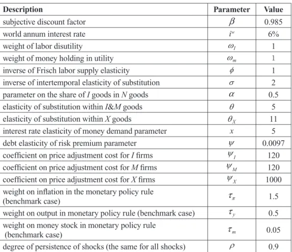
after excluding investment, and adjusting so that in the steady state the home country is owing some debt to the foreign country, but it is also running a trade account surplus in or-der to pay exactly the debt service so that the debt-GDP ratio is kept constant. With these data, it is possible to pin down the basic structure of the model economy. Other parameters are set as shown in Table 2. Most of the values are quite standard in the literature, see for example Devereux et al. (2006). The subjective discount factor is 0.985 which implies an annum interest rate of 6% of the home country at the steady state. This, the debt-GDP ra-tio in Table 1, and the world interest rate imply a value of 0.0097 for the debt elasticity of risk premium parameter. The coefficient on price adjustment cost for X firms is set to be very high to capture the fact that the export price denominated in the foreign currency is almost fixed and given to an emerging country like Thailand. The degree of persistence of structural shocks is 0.9, a quite high value, and is the same for all shocks.
Below we will analyze the simulation results. Although we have introduced into the model six types of shocks and the model is flexible enough to deal with many different situations in reality, we only pick up several cases due to the limited space. We will refer as the benchmark case to the case in which export firms practice LCP, exchange rate pass-through to import price is mild ( M=120), and the central bank follows a Taylor rule to conduct monetary policy.
Table 1: Structure of aggregate demand and external debt of Thailand (average of 2000-2009)
Indicators
(as ratio to GDP) Actual data
Values used in simulation (after adjusting to be consistent with
the steady state of the model)
private consumption 0.56 0.79
government consumption 0.12 0.21
gross domestic capital formation 0.26
-exports of goods and services 0.70 0.77
imports of goods and services 0.64 0.76
external debt 0.43 0.43
Table 2: Parameter values set for simulation
Description Parameter Value
subjective discount factor 0.985
world annum interest rate iw 6%
weight of labor disutility I 1
weight of money holding in utility m 1
inverse of Frisch labor supply elasticity 1
inverse of intertemporal elasticity of substitution 2
parameter on the share of I goods in N goods 0.5
elasticity of substitution within I&M goods 5
elasticity of substitution within X goods X 11
interest rate elasticity of money demand parameter x 5
debt elasticity of risk premium parameter 0.0097
coefficient on price adjustment cost for I firms I 120 coefficient on price adjustment cost for M firms M 120 coefficient on price adjustment cost for X firms X 1000 weight on inflation in the monetary policy rule
(benchmark case) 1.5
weight on output in monetary policy rule (benchmark case) y 0.5 weight on money stock in monetary policy rule
(benchmark case) m 0.05
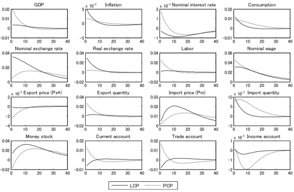
Figure 1: Effects of a decrease in the domestic nominal interest rate under PCP and LCP
(monetary policy rule is a Taylor rule)
Effects of shocks under PCP and LCP on the export side
We first consider how different the effects of shocks are under different international price settings. Figure 1 presents the effects of a negative shock to the domestic nominal interest rate under LCP and PCP on the export side. We could see that, compared to the PCP case, under LCP the export price denominated in the foreign currency (Pt*(x)) is very rigid (i.e.
exchange rate pass-through to Pt*(x) is very small), and as a result, export quantity remains
unchanged, and thus GDP does not change much, so the central bank does not raise the nominal interest rate much. As a result, the exchange rate depreciates more, which in turn raises import price (Pt(m)) causing inflation to rise more. In addition, under the LCP case exports do not change much while imports increase, so the trade account and thus the cur-rent account deteriorate. Under PCP we observe the opposite.
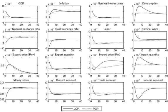
Figure 2: Effects of an increase in demand for home export abroad under PCP and LCP
(monetary policy rule is a Taylor rule)
Figure 2 shows the effects of a shock that increases the demand for exports of the home country abroad under LCP and PCP. We observed that, under LCP since the export price denominated in the foreign currency (Pt*(x)) is very rigid, the increase in foreign demand is
met by an increase in export quantity, which raises the trade account, the current account, and GDP. The central bank responds to the increase in GDP above its steady state level by raising the interest rate, thus the nominal exchange rate appreciates. Import price falls as a result, which exceeds the effect of increasing wages due to the increase in labor demand of export firms, so inflation falls. Under PCP, because Pt*(x) is not rigid, the increase in
foreign demand is almost met by an increase in Pt*(x), so the effects on other variables are
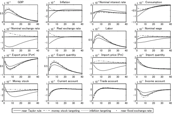
Figure 3: Effects of a decrease in the domestic nominal interest rate under different monetary policy rules (export firms practice LCP)
Effects of shocks under different monetary policy rules
Figure 3 shows the effects of a negative shock to the domestic nominal interest rate under different monetary policy rules. Under a fixed exchange rate regime, the central bank acts to keep the nominal interest rate unchanged (to maintain the fix) and thus the effects on the current account and other variables are negligible. In contrast, under a Taylor rule the shock causes inflation, GDP and thus consumption to increase, and the nominal exchange rate to depreciate. As a result, export price (Pt*(x)) falls, export quantity increases, while
import price (Pt(m)) goes up which raises inflation further and at the same time works to reduce import quantity. But the effect of the increase in GDP is larger so import quantity rises, worsening the trade account and current account. Under inflation targeting, we can see that the central bank responds very strongly to the increase in inflation so the nominal interest rate turns to rise. However, under this rule and the money stock targeting rule, the effects of the shock on the current account and other variables are small.
Figure 4: Effects of an increase in government spending under different monetary policy rules
(export firms practice LCP)
In Figure 4, an increase in government spending causes GDP to rise and consumption to fall. The latter result is well known in the literature: the government raises tax to finance its increased consumption, thus reducing the disposal income of households and their consumption. Households respond to this fall in consumption by working more, thus labor supply increases and wages go down. Under the Taylor rule, the exchange rate appreci-ates, making import price cheaper and thus inflation goes down. Due to the increase in GDP and the fall in import price, import quantity increases which dominates the increase in export quantity (because export price falls as a result of the fall in wages) resulting in a deterioration of the trade and current account.
Figure 5: Effects of an increase in TFP of the export sector under different degrees of exchange rate pass-through to import price (export firms practice LCP, monetary policy rule is a Taylor rule)
Effects of shocks under different degrees of exchange rate pass-through to import price
Figure 5 shows the effects of an increase in the TFP of the export sector under different values of the coefficient on the price adjustment cost for M firms ( M) which governs the degree of exchange rate pass-through to import price. The shock increases GDP and con-sumption and thus raising imports. The nominal exchange rate appreciates, which contrib-utes further to push up imports. On the other hand, the shock allows export firms to reduce their prices to some extend, which raises exports. The simulation result shows that the increase in exports is larger than the increase in imports so the trade account and current account improve.
4. Concluding Remarks
We have examined the effects of various types of structural shocks to the current account in a New Keynesian small open economy model. We find that in many cases the qualitative and quantitative effects of a shock depend on factors such as monetary policy rules and the degree of exchange rate pass-through on both import and export sides. Since our re-sults so far have been drawn from a model calibrated to the data of Thailand, a highly open economy, it important to check whether these results also hold for less open economies. In addition, we have considered only the case of temporary (but persistent) shocks since our focus here is the short run, it is, however, interesting to investigate the case of permanent shocks which allows us analyze the dynamics of the current account in the longer run. It is also worth analyzing the case where the home country uses imported goods as interme-diates for the production of exported goods, as is observed in many East Asian countries which participate in the so-called intra-regional production networks. I plan to investigate further along these lines in future work.
References
Asian Development Bank (ADB), Key Indicators for Asia and the Pacific 2010, available from www.adb.org/statistics.
Devereux, B. Michael, Philip R. Lane, and Juanyi Xu (2006), “Exchange rate and mon-etary policy in emerging market economies,” The Economic Journal, 116, 478-506. Dynare, available from www.dynare.org.
Schumitt-Grohe, Stephanie and Martin Uribe (2003), “Closing small open economy mod-els,” Journal of International Economics, 61, 163-185.
Shioji, Etsuro, Vu Tuan Khai, and Hiroko Takeuchi (2009), “Shocks and Incomplete Ex-change Rate Pass-through in Japan: Evidence from an Open Economy DSGE Model,” paper presented at the Far East and South Asia Meeting of the Econometric Society, University of Tokyo, August 2009.