Heping PENG*
,**, Zhuoqun PENG*** and Zhipeng ZHOU*
*School of Mechatronics and Automation, Wuchang Shouyi University, Wuhan 430064, China E-mail: hbjhun_penn@outlook.com
** School of Intelligent Manufacturing, Jianghan University, Wuhan 430056, China
***School of Machinery and Automation, Wuhan University of Science and Technology, Wuhan 430065, China
Received: 14 October 2020; Revised: 24 February 2021; Accepted: 26 April 2021 Abstract
The aim of this paper is to study the modeling method of the geometric variations which occur at the successive set-ups of the machining process by relying on the small displacement torsor (SDT) and its transfer formula, and to develop the machining process evaluation method based on the limitation of functional tolerances. The proposed method firstly considers the machining process of the mechanical part as a mechanism mainly consisted of machine-tool, part-holders, machined part, and cutting tools; Then, the SDT parameters are employed to represent the geometrical variations of the part caused by the positioning errors and machining operations during successive machining set-ups; the SDT chains are used to model the deviation propagation between different set-ups. During the whole modeling, there are three kinds of torsors need to be defined which are the global SDT of the part-holder, machined part or machining operation relative to their respective nominal positions, the gap torsor between two contact surfaces, and the deviation torsor of the associated surface relative to their respective nominal positions on the part-holder, machined part or machining operation. After obtaining all SDT chains based on the process planning of the part, an evaluation method is developed to verify the effectiveness of machining process by cumulating the impacts of various manufacturing variations on the respect of functional tolerances. Finally, an example is given to illustrate how to use the proposed method to model the manufacturing variations and evaluate the machining process of the part in the field of CNC milling machining.
Keywords : Manufacturing variation modeling, Process evaluation, Machining tolerancing, Small displacement
torsor (SDT), Functional tolerance
1. Introduction
Tolerance is the concrete reflection of product precision, the outcome of coordination between product requirements and development costs, and an important technical indicator in the processes of product design, manufacturing, verification, assembly, and testing (Zhong et al., 2013), (Qin et al., 2018). The manufacturing process of a part is usually composed of multiple set-ups; process parameters in each set-up will have impacts on the product quality; modeling the machining variations of the part in the successive set-ups of the machining process and discussing 3D transfer techniques of manufacturing tolerance are of great practical significance for reducing the manufacturing cost and improving the machining quality of the part. The tolerance transfer technique is to explore how to convert design tolerances into manufacturing tolerances in the product process planning stage (Thimm et al., 2007). The traditional tolerance transfer technique is to make use of the tolerance charting, which enables process planners to obtain manufacturing tolerances according to design tolerances for each processing operation. The early researches mainly focus on the one-dimensional tolerance charting method to determine the working dimensions and tolerances in process planning (Ji, 1993), (Ngoi and Tan, 1997). Later, Xue and Ji (2004) extended one-dimensional method to two-dimensional tolerance charting. However, tolerance charting techniques can only deal with the size-dimensional tolerances or a limited set of geometric tolerances (Wang et al., 2010). In order to consider the influence of geometric process variations, Bourdet and Ballot (1995) proposed a three-dimensional variations model by using the small displacement torsor (SDT) to model geometric deviations in manufacturing process. The SDT model is a mathematical
Manufacturing variation modeling and process evaluation based on
small displacement torsors and functional tolerance requirements
components. Since then, the concept of SDT has been widely used in the study on the tolerancing techniques in the areas of product design and process planning. Based on the concept of SDT, Legoff et al. (1999) put forward a method for performing tridimensional analysis and synthesis of machining tolerances. By using the SDT parameters to characterize the variations of the machining operations, the part-holder and the workpiece, Villeneuve et al. (2001) presented 3D model of manufacturing tolerances. Vignat and Villeneuve (2003) used the SDT approach to perform three-dimensional manufacturing tolerancing for turning operation. Legoff et al. (2004) introduced two approaches of three-dimensional manufacturing errors modeling and the comparative analysis of two approaches has been done as well. In addition, Villeneuve and Vignat further extended the SDT-based method to tolerance synthesis (Villeneuve and Vignat, 2003), (Villeneuve and Vignat, 2005). Anselmetti and Louati (2005) have proposed a graphical representation of part features, process plans and functional requirements to analyze these three-dimensional specifications and to generate manufacturing specifications with ISO standards. Louati et al. (2006) proposed a machining tolerancing method using SDT theory to optimize a manufactured part setting. Ayadi et al. (2008) adopted the SDTs to represent the variation defects between manufactured surfaces and nominal surfaces of the workpiece and proposed a 3D modeling method of manufacturing tolerancing. In order to realize the transfer from functional tolerances to manufacturing ones, Villeneuve and Vignat (2005) presented a model of manufactured part (MoMP) to model successive manufacturing processes which takes into account the geometrical and dimensional deviations produced with each machining setup and the influence of these deviations on further setups. Using the SDT as a tool to describe the surface defects and the MoMP as an approach to determine the stack-ups of these defects in the multi-stage manufacturing process of a part, Nejad et al. (2009) developed a model to cumulate the impacts of various sources of manufacturing errors and realize tolerance analysis. Nejad et al. (2012) have also compared the three different solution techniques which are developed by the authors for simulating the manufacturing process in order to perform the tolerance analysis in the multi-stage machining process. Abellán-Nebot et al. (2013) analyzed two 3D manufacturing variation models, that is the stream of variation model (SoV) and model of the manufactured part (MoMP), in multi-station machining systems and compared their main characteristics and applications. Anselmetti (2012) presented a three-dimensional transfer method using the analysis line method to generate a relationship giving the three-dimensional result of the tolerance chain as a linear function of tolerances of manufacturing specifications. Royer and Anselmetti (2016) also put forward the 3D transfer method of manufacturing tolerances, in which SDTs are employed to model the machining deviations and the analysis line method is used to obtain the transfer relations between functional tolerances and manufacturing tolerances. Furthermore, Laifa et al. (2014) presented a 3D formalization of manufacturing tolerancing which associates the concept of SDTs, the functional constraints, and manufacturing process capability. This approach enables the evaluation of manufacturing process by limiting the variations which occur at the various production setups. Zhang and Qiao (2013) presented 3D manufacturing tolerance design method by using SDT to establish the algebra model of 3D tolerance zone, and using convex sets theory to calculating and optimizing the 3D tolerance zone.
This paper aims at 3D modeling techniques of the geometrical variations in the machining process of the part using the SDT and its transfer formula, and exploring the evaluation method of the machining process. The first part introduces the concept of SDT and its transfer formula; The second part discusses 3D modeling techniques for manufacturing variations and deviation propagation, in which SDT parameters are employed to model all variations in the successive set-ups of the machining process regardless of the causes of these variations and the SDT chains are used to model the deviation propagation between different set-ups; The third part develops the method of machining process evaluation by simulating the influence of the manufacturing variations on the respect of functional tolerance requirements; Finally, an example shows the application of the proposed method in the field of CNC milling machining.
2. Small displacement torsor and its transfer formula
As we know, any variation of a geometrical feature from its nominal position can be characterized by the SDT with three rotation components (α, β, γ) around x, y, z axes and three translation components (u, v, w) along x, y, z axes, respectively (Peng and Lu, 2018). The SDT { } { }
i i
i
i/P (O,R) O
P ε
τ , which synthesizes the position and orientation of an associated feature Pi relative to its nominal feature at a given point Oi in a local reference frame Ri, can be expressed as (Teissandier et al., 1999):
) R , O ( O ) R , O ( /P P i i i i i i w γ v β u α } { } { ε τ (1)
For special cases, the variation torsor of a cylindrical associated feature Pi with regard to its nominal cylinder can be expressed as: ) ,R (O O ) ,R (O /P P i i i i i i w γ v β U U } { } { ε τ (2)
where point Oi belongs to the cylinder and Ri is a local reference frame whose axis xi coincides with the axis of the cylinder, capital U represents the undetermined component in the expression of a torsor.
Similarly, the variation torsor of a plane feature Pi can be expressed as:
) R , O ( O ) R , O ( /P P i i i i i i w U U β U α } { } { ε τ (3)
where point Oi belongs to the plane and Ri is a local reference frame whose axis zi is the normal of the plane.
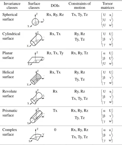
According to the new generation Geometrical Product Specifications and Verification (GPS) system, the geometries of parts are divided into seven invariance classes. Each invariance class has the corresponding Degree of Invariance (DOI), and it is a set of ideal features with the same DOI. If the characteristics remain intact when a feature translates along x, y, z axes or rotates around these axes, the characteristic invariance of corresponding direction is called DOI. For example, the cylinder invariance class keeps characteristics unchanged when it translates along axis x and rotates around this axis, its DOI is 2 (Tx, Rx). Table 1 lists seven invariance classes, their DOIs and torsor matrices.
Table 1 Seven invariance classes in the new generation GPS system (Peng and Lu, 2018)
Invariance classes Surface classes DOIs Constraints of motion Torsor matrices Spherical surface Rx, Ry, Rz Tx, Ty, Tz w U v U u U Cylindrical surface Rx, Tx Ry, Rz Ty, Tz w v U U Planar surface Rz, Tx, Ty Rx, Ry, Tz w U U U Helical surface Rx, Tx Ry, Rz Ty, Tz w v U U Revolute surface Rx Ry, Rz Tx, Ty, Tz w v u U Prismatic surface Tx Rx, Ry, Rz Ty, Tz w v U Complex surface 0 Rx, Ry, Rz Tx, Ty, Tz w v u
In order to facilitate the operation of torsors, the following two properties are defined (Villeneuve et al., 2001): Property 1: R a , aUU (4) Property 2: 2 R b , a , aUbUU (5) Suppose { } { } i i i i/P (O,R) O P ε
τ is a torsor at point Oi in a local reference frame Ri, then torsor {τPi/P}(O,R0) at point O expressed in the global reference frame R0 can be expressed as:
( ( OO) )
} { i T ,i 0 O i , 0 ,i ) R , O ( /P Pi R R i R τ 0 0 (6)where R0,i is the rotation matrix from R0 to Ri,
T i , 0
R is the transposed matrix of R0,i, and vector OOi is the
translation vector from R0 to Ri expressed in R0.
If there is only translation transformation between R0 and Ri, the above transfer formula will be simplified as:
O i ) R , O ( /P P } OO { i i 0 τ (7)3. Modeling of the manufacturing variations
The machining process of a part is generally composed of different set-ups, each set-up can be considered as a mechanism mainly consisted of machine-tool, part-holders, machined part, and cutting tools. We suppose that the geometrical variations in the machining process are small enough to be modeled with SDT.
3.1 Modeling of the geometrical variations
In order to model all manufacturing variations, three types of torsors need to be defined, namely the global variation SDT of the part-holder or machined part relative to their respective nominal positions, the deviation SDT of real surface of the part-holder or machined part relative to their respective nominal surfaces, and the gap SDT between two contact surfaces.
The global variation SDT
For set-up Sk, the global variation SDT associated with the machined part, the part-holder, and the machining operation are defined respectively:
k
S P/R
τ : global variation SDT of the machined part P characterizes the positioning variations of the machined part with respect to its nominal position in set-up Sk.
k
S H/R
τ : global variation SDT of the part-holder H relatively to its nominal position in set-up Sk.
k
S M/R
τ
: global variation SDT of the machining operation M characterizes variations of a machine-tool relatively to its nominal position in set-up Sk. The deviation SDT
For set-up Sk, the deviation SDT associated with the machined part, the part-holder, and the machining operation are defined respectively: k i S /R P
τ : deviation SDT of the machined surface Pi with regards to its nominal position in set-up Sk (variations of the machining operation).
/P Pi
τ : deviation SDT expresses the orientation and position variations of surface Pi relatively to its nominal position on part P. Suppose surface Pi is manufactured in set-up Sk, this deviation torsor can be calculated as:
k k i i S P/R S /R P P P τ τ τ / (8) k i S /H H
τ : deviation SDT expresses the geometric variations of surface Hi relatively to its nominal position on part-holder in set-up Sk. k i S /M M
τ : deviation SDT expresses the geometric variations of surface Mi relatively to its nominal position on the machining operation M in set-up Sk.
Considering the identity between the surface of the machining operation and the surface machined on the part, we also have: k k i k i k i S R M S M M S R M S /R P τ / τ / τ / τ (9) The gap SDT k i i S /H P
τ : gap SDT which expresses the variations of the interface between surface Pi of the machined part and the corresponding surface Hi of the part-holder in set-up k. Given that the parts do not interpenetrate at the contacts, each fixed component of the torsors is regarded as nil.
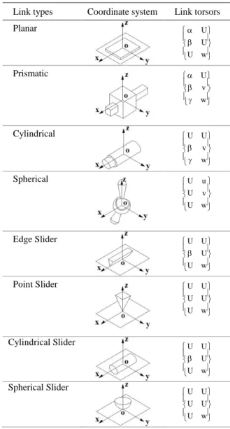
The main link types of the interfaces between the machined surfaces and the positioning surfaces in machining operations and corresponding torsors are list in Table 2. The undetermined components in the link torsors are denoted by “U”, which show the components that leave the characteristic invariance of corresponding direction.
Table 2 Main link types and the corresponding torsors
Link types Coordinate system Link torsors
Planar w U U U Prismatic w v U Cylindrical w v U U Spherical w U v U u U Edge Slider w U U U U Point Slider w U U U U U Cylindrical Slider w U U U U Spherical Slider w U U U U U The SDT chain
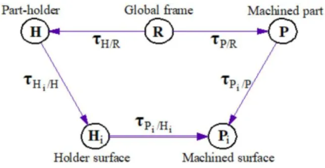
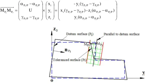
The machining process of the part is the process of constantly creating new surfaces. The developed manufacturing variation model regards each machining set-up as a mechanism consisting of a machine-tool, several machining operations, a machined part and its surface, and a part-holder and its surface. As shown in Fig. 1, for any set of two interacting surfaces (Pi, Hi), we can obtain the SDT chain as follows:
/H H H/R P/R /P P /H Pi i τ i τ - τ -τ i τ (10)
Fig. 1 The SDT chain of contact surfaces
3.2 Variation propagation between different set-ups
The machining process of a part generally consists of several different set-ups, and we will discuss how these geometrical variations are propagated between set-ups.
It is assumed that torsor
τ
Pb/Pa can represent the functional tolerance between two machined surfaces Pa and Pb of part P, and its expression is as follows:/P P /P P P/P /P P /P Pb a
τ
bτ
aτ
b- τ
aτ
(11)Suppose surfaces Pa and Pb are machined in set-ups S1 and S2 respectively, according to Eqs. (8) and (10), Eq. (11) becomes: ) ( ) ( 1 1 i 1 i i i 1 a 2 2 i 2 i i i 2 b a b S H/R S /H H S /H P /P P S /R P S H/R S /H H S /H P /P P S /R P /P P τ τ τ τ τ τ τ τ τ τ τ (12)
Thus, the relationship between functional tolerances and various variations in each set-up can be established to reveal how geometric variations are propagated between different set-ups. This relationship can further guide the process engineers to evaluate the machining process.
4. Evaluation of the machining process
In this section, we will develop the evaluation method to verify the effectiveness of the multi-stage manufacturing process based on the limitations on the manufacturing variations by several geometric tolerances related to functional requirements, such as flatness tolerance, parallelism tolerance, position tolerance, perpendicularity tolerance, etc. (see Fig. 2).
4.1 Flatness tolerance requirement
As shown in Fig.2, the flatness tolerance of flat surface P1 indicates that the actual surface P1 shall be contained between two parallel planes a distance Tpl apart.
One uses the torsor to model the variations of surface P1 with regard to its nominal position in the global reference frame R0: U v U U } { /P P /P P /P P ) R , O ( /P P 1 1 1 0 1 τ (13)
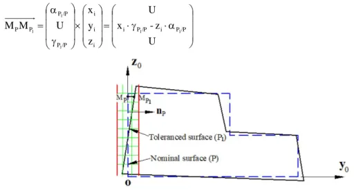
As shown in Fig. 3, the variation of tolerance plane P1 with regard to its nominal position is defined by the displacement of any point of the tolerance plane MP1 compared to the corresponding point MP. Since the displacement depends only on the rotation variations, it can be calculated as:
U z -x U z y x U M M i P/P i P/P i i i /P P /P P P P 1 1 1 1 1 (14)
Fig. 3 Variations between toleranced plane and datum plane To satisfy the flatness tolerance requirement, one has:
pl P P PM n T M 1 (15) where 0 1 0
nP is the normal vector to the nominal plane P. By neglecting the higher-order terms beyond the first
order, inequality (15) becomes: pl /P P i /P P i
-
z
T
x
1 1
(16)4.2 Parallelism tolerance requirement
As shown in Fig.2, the parallelism tolerance of flat surface P7 related to datum surface A (P1) indicates that the actual plane P7 shall be contained between two parallel planes Tpa apart which are parallel to datum plane A.
Similarly, the variation torsor of machined plane P7 with regard to its nominal surface in the global reference frame R0: U v U U } { /P P /P P /P P ) R , O ( /P P 7 7 7 0 7 τ (17)
U v v U U } { -} { } { /P P /P P /P P /P P /P P /P P ) (O,R /P P ) (O,R /P P ) (O,R /P P 1 7 1 7 1 7 0 1 0 7 0 1 7 τ τ τ (18)
As shown in Fig.4, the variations of toleranced surface P7 relative to datum surface P1 is defined by the displacement of any point of the tolerance surface MP7 compared to the point corresponding MP1. Since the displacement depends only on the rotation variations, it can be calculated as:
) ( y ) ( z -) ( x ) ( y -z y x U M M /P P /P P i /P P /P P i /P P /P P i /P P /P P i i i i /P P /P P /P P /P P P P 1 7 1 7 1 7 1 7 1 7 1 7 7 1 (19)
Fig. 4 Variations between toleranced surface and datum surface To satisfy the parallelism tolerance requirement, one gets:
pa P P PM n T M 1 7 1 (20) where P / P P / P P 1 1 1 -1
n is the normal vector to the datum plane A. By neglecting the higher-order terms beyond the first
order, inequality (20) becomes:
pa /P P /P P i /P P /P P i( )-z ( ) T x 1 7 1 7 (21)
4.3 Position tolerance requirement
As shown in Fig.2, the position tolerance of flat surface P7 related to datum surface A (P1) indicates that the actual plane P7 shall be contained between two parallel planes Tpo apart which are symmetrically disposed about the theoretically exact position of the flat surface with respect to datum plane A.
The same as the parallelism tolerance requirement, the variations of toleranced surface P7 relative to datum surface P1 is defined by the displacement of any point of the tolerance surface MP7 relative to the point corresponding MP1 (see Fig.4); But for position tolerance requirement, the difference is that the displacement depends on rotation and translation variations at the same time, so it can be calculated as follows:
U v -v ) ( z -) ( x U z y x U U v -v U M M i P/P P/P i P/P P/P P/ P P/P i i i /P P /P P /P P /P P P / P P / P P P 7 1 7 1 7 1 1 7 1 7 1 7 7 1 (22)
So to satisfy the position tolerance requirement, one gets: 2 T n M MP P P po 1 7 1 (23) Similarly, by neglecting the higher-order terms beyond the first order, inequality (23) becomes:
2 T v -v ) ( z -) ( xi P7/PP1/P i P7/PP1/P P/7P P1/P po (24)
4.4 Perpendicularity tolerance requirement
As shown in Fig.2, the perpendicularity tolerance of surface P8 related to datum surface B (P7) indicates that the actual surface P8 shall be contained between two parallel planes Tpe apart that are perpendicular to datum plane B.
One uses the torsors to model the variations of machined surface P8 related to datum surface B (P7) in the global reference frame R0: U U U U U -U v U U -w U U U } { -} { } { P / P P / P P / P P / P P / P P / P P / P P / P ) R , O ( /P P /P P ) R , O ( /P P 7 8 7 7 7 8 8 8 0 7 ) 0 R , O ( 8 0 7 8 τ τ τ (25)
As shown in Fig.5, the variations of toleranced surface P8 relative to datum surface P7 is defined by the displacement of any point of the tolerance surface MP8 compared to the corresponding point MP7 of the situation surface perpendicular to the datum surface P7. Since the displacement also depends only on the rotation variations, it can be calculated as: ) ( y ) ( z -U z y x U U M M /P P /P P i /P P /P P i i i i /P P /P P P P 7 8 7 8 7 8 8 7 (26)
Fig. 5 Variations between toleranced surface and situation surface Similarly, to satisfy the perpendicularity tolerance requirement, one has:
pe P P PM n T M 7 8 7 (27) where 1 -n P/P P / P P 7 7 7
is the normal vector to the situation plane perpendicular to datum surface P7. By neglecting the
higher-order terms beyond the first order, inequality (27) becomes: pe /P P /P P i( ) T y 7 8 (28)
5. Application to CNC milling process
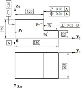
In this section, an example (see Fig. 6) is given to illustrate the application of the proposed method in the field of CNC milling machining. The functional tolerance requirements of the part include the flatness tolerance of flat surface P1, the position and the parallelism of plane P7 with respect to datum A on plane P1, the perpendicularity of plane P8 with respect to datum B on plane P7 as described in Fig. 6. And Figs.7-9 show the machining process of this part, which consists of three set-ups performed on a computer numerical control (CNC) machine-tool.
Fig. 6 Machined part geometry
5.1 Set-up 10
In set-up 10, a rectangular cube raw material will be used; the six surfaces of the raw material will be carried out the rough machining, that is, there are no positioning surfaces. In the global reference frame R0 (O, x0, y0, z0) shown in Fig. 7, the machined surfaces are marked as Pi, the local reference frame Ri (Oi, xi, yi, zi) for each machined surface is defined as: Axis zi is normal to surface Pi pointing towards the outside of the entity; Origin Oi, axes xi and yi of the reference frame belong to surface Pi, we have:
i i i i i i P P P P P P R O /P P w U U β U α ) , ( } {τ , i{1,2,6}
Fig.7 Set-up10: Rough machining of surfaces
5.2 Set-up 20
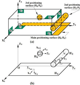
Taking into account the tolerance specifications of the machined part, surface P1 of the part is carries out the milling machining in set-up 20. During the milling process, the machined part is located by a plane, a cylindrical surface and a spherical surface in an isostatic positioning setting; in which the contact planar H4/P4 acts as the main positioning surface, the cylindrical slider H2/P2 with radius rc acts as the 2
nd
positioning surface; the spherical slider H6/P6 with radius rs acts as the 3rd positioning surface, as shown in Fig. 8. Here, the coordinate origin of the local frame
) z , y , x , o (
Ri i i i i , i{2, 4,6}, is set at the contact point between the part-holder Hi and positioning plane Pi, denoted as Oi. Next, we derive the global torsor τ
20
P/R based on the torsor expression in relation with the contact surfaces between part-holder Hi and part Pi.
Fig. 8 Set-up20: Milling of surface P1
As shown in Fig. 8(b), in the local frame Ri (Oi, xi, yi, zi), i∈{2, 4, 6}, assuming that the global SDT
k
S H/R
τ of
part-holder is nil, according to the torsor matrices of invariance classes on Table 1, one get:
20 H H H 20 H H 20 H ) ,R (H 20 4 4 4 4 4 /H 4 H w U U β U α } {τ , 20 H 20 H 20 H 20 H H H ) ,R (H 20 /H H 2 2 2 2 2 2 2 w γ v β U U } {τ , 20 H H 20 H H 20 H H ) ,R (H 20 /H H 6 6 6 6 6 6 w U v U u U } {τ
We use Eq. (7) to calculate torsors
) ,R (O 20 /H Hi } i i
{τ ,i{2,4,6}, in which the translation vectors from {R }
i
H to {ROi}
are H2O2(0,0,-rc), H4O4(0,0,0) and H6O6(0,0,-rs), respectively. So for these three positioning surfaces, one
will have: 20 H H H 20 H H 20 H ) ,R (H 20 ) ,R (O 20 4 4 4 4 4 /H 4 H 4 4 /H 4 H w U U β U α } { } {τ τ , 20 H 20 H H c 20 H 20 H 20 H c H H ) ,R (O 20 /H H 2 2 2 2 2 2 2 2 w γ U r v β β -r U U } {τ , 20 H H H s 20 H H H s 20 H H ) ,R (O 20 /H H 6 6 6 6 6 6 w U U r v U U -r u U } {τ
Then we can calculate the torsors 20 (O,R ) /P Pi } 0
{τ and 20 (O,R ) /H Hi } 0
{τ i{2,4,6} at point O expressed in the global reference frame R0 (O, x0, y0, z0) by using Eq. (6), suppose the origin coordinate of the local reference frame Ri is Oi (ai, bi, ci), i{2,4,6} (see Fig.7), the rotation matrices R0,i from R0 to Ri respectively are:
0 1 0 1 0 0 0 0 1 2 , 0 -R , 1 -0 0 0 1 -0 0 0 1 4 , 0 R , 0 0 1 0 1 0 1 -0 0 6 , 0 R We get: 4 4 4 4 4 4 4 0 4 P 4 P 4 P P P 4 P 4 P P P 4 P 4 P P ) (O,R /P P α -b β -a -w -U α c U a -U -β β c U -b U α } {τ , 2 2 2 2 2 2 2 0 2 P 2 P 2 P P P 2 P 2 P P P 2 P 2 P P ) (O,R /P P α b U a U β α c β a w U β b U c U α } { -τ
6 6 6 6 6 6 6 0 6 P 6 P 6 P P P 6 P 6 P P P 6 P 6 P P ) (O,R /P P β a U b U α α -a U -c U β α b β -c -w -U } {τ , 20 H 4 20 H 4 20 H H 20 H 4 H 4 H 20 H 20 H 4 H 4 H 20 H ) (O,R 20 /H H 4 4 4 4 4 4 4 0 4 α -b β -a -w -U α c U a -U -β β c U -b U α } {τ H 2 20 H 2 H c 20 H 20 H H 2 20 H 2 20 H 20 H 20 H 2 20 H 2 20 H c H H ) (O,R 20 /H H U -b γ a U -r -v -β U c β a w γ β -b γ -c β -r U U } { 2 2 2 2 2 2 2 2 2 0 2 τ , H 6 H 6 H s 20 H H H 6 H 6 H s 20 H H H 6 H 6 20 H H ) R , O ( 20 H / H U a U b U -r u U U -a U -c U r v U U c U b -w -U } { 6 6 6 0 6 -τ
According to Eq. (10), we can get the gap SDT (O,R) 20
/H Pi i} 0
{τ at point O expressed in global reference frame R0 (O, x0, y0, z0). 20 H 4 20 H 4 20 H 20 H 20 P P 4 P 4 P H 20 H 20 P P 20 H 4 H 4 H 20 H 20 P P 4 P 4 P 20 H 20 H 20 P P 20 H 4 H 4 H 20 H 20 P P 4 P 4 P 20 H 20 H 20 P P ) (O,R 20 /H P 4 4 4 4 4 4 4 4 4 4 4 4 4 4 0 4 4 α b β a w -w w α -b β -a -w U -γ γ -U α -c U -a U -v v α c U a -U β -β β -β β -c U b -U -u u β c U -b U -α -α α α } {τ H 2 20 H 2 H c 20 H 20 H 20 P P 2 P 2 P 20 H 20 H 20 P P H 2 20 H 2 20 H 20 H 20 P P 2 P 2 P 20 H 20 H 20 P P 20 H 2 20 H 2 20 H c H 20 H 20 P P 2 P 2 P H 20 H 20 P P ) (O,R 20 /H P U b γ -a U r v -w w α -b U a -U β -γ γ -β U -c β -a -w -v v α c β a w -γ -β β U β b γ c β r -U -u u β -b U -c U -U -α α α } { 2 2 2 2 2 2 2 2 2 2 2 2 2 2 2 2 0 2 2 τ H 6 H 6 H s 20 H 20 H 20 P P 6 P 6 P H 20 H 20 P P H 6 H 6 H s 20 H 20 H 20 P P 6 P 6 P H 20 H 20 P P H 6 H 6 20 H 20 H 20 P P 6 P 6 P H 20 H 20 P P ) (O,R 20 /H P U -a U -b U r -u -w w β a U b U -U -γ γ α U a U c U -r -v -v v α -a U -c U -U -β β β U c U -b w -u u α b β -c -w U -α α -U } { 6 6 6 6 6 6 6 6 6 6 0 6 6 τ Suppose {τPi/Hi}(O,R0){ εO} then,
R R (ε OO)
} { O i T i , 0 T i , 0 ) R , O ( H / Pi i i i τ (29)In the local frame Ri(oi,xi,yi,zi), the gap SDT (O,R) 20
/H Pi i} i i
{τ at point Oi can be derived using Eq. (29), and in combination with the properties (4) and (5) of torsor, one will get:
20 H 4 20 P 4 20 H 4 20 P 4 20 H 20 H 20 P P 20 H 20 H 20 P P 20 H 20 H 20 P P ) ,R (O 20 /H P β -a β a α b α -b -w w -w w U U -β β -β β U -α -α α α } { 4 4 4 4 4 4 4 4 4 4 τ 20 H 2 20 P 2 20 H 2 20 P 2 20 H 20 H 20 P P 20 H 20 H 20 P P ) ,R (O 20 /H P γ -a γ a α c α c -w -v v w U U β γ γ β U U } { 2 2 2 2 2 2 2 2 -τ 20 H 6 20 P 6 20 H 6 20 P 6 20 H 20 H 20 P P ) ,R (O 20 /H P γ -b γ b β c β -c -w u -u w U U U U U } { 6 6 6 6 6 6 τ
Considering the hierarchy of the part/part-holder positioning in the isostatic setting, the components of (O,R) 20
/H P4 4} 4 4
{τ
are nil because the contact between the two main positioning surfaces (H4/P4) has no interpenetrating parts. One gets the following equations: 0 β a β a α b α b w w w w 0 β β β β 0 -α -α α α 20 H 4 20 P 4 20 H 4 20 P 4 20 H 20 H 20 P P 20 H 20 H 20 P P 20 H 20 H 20 P P 4 4 4 4 4 4 --
0 γ -a γ a α c α c -w -v v w 0 β γ γ β 20 H 2 20 P 2 20 H 2 20 P 2 20 H 20 H 20 P P 20 H 20 H 20 P P 2 2 2 2 -0 γ b γ b β c β c w u u w 20 H 6 20 P 6 20 H 6 20 P 6 20 H 20 H 20 P P6- - 6- - Then, (O,R) 20 P/R} 0
{τ can be derived as:
20 H 4 P 4 20 H 4 P 4 20 H 20 H P 20 H 20 H P 20 H 2 P 2 20 H 2 P 2 20 H 20 H P 20 H 20 H P 20 H 6 P 6 20 H 6 P 6 20 H 20 H P 20 H 20 H P ) R , O ( 20 P/R 4 4 4 4 4 4 2 2 2 2 4 4 2 2 4 4 2 2 4 4 6 6 4 4 0 β a β a α b α b w w w β γ β β a β a α c α c w v w β β β β b β b β c β c w u w α α α } { -τ
Using Eq. (29), we get:
20 H 1 20 H 1 P 1 20 H 1 20 H 1 P 1 20 H 2 P 2 20 H 2 P 2 20 H 20 H P 20 H 20 H P 20 H 1 20 H 1 P 1 20 H 1 20 H 1 P 1 20 H 4 P 4 20 H 4 P 4 20 H 20 H P 20 H 20 H P 20 H 1 20 H 1 P 1 20 H 1 20 H 1 P 1 20 H 6 P 6 20 H 6 P 6 20 H 20 H P 20 H 20 H P ) ,R (O 20 P/R 2 2 4 4 2 2 4 4 2 2 4 4 4 4 4 4 4 4 4 4 4 4 2 2 2 2 4 4 2 2 4 4 6 6 4 4 1 1 β a γ a β a α c α c α c β a β a α c α c w v w β β β β a β a β a α b α b α b β a β a α b α b w w w β γ β β b γ b β b β c β c β c β b β b β c β c w u w α α α } { -τ As τ1 ( 1, 1) τ1 ( 1, 1) τ (O1,R1) 20 P/R R O 20 /R P R O /P P } { } -{ }
{ and combining the properties of torsor, the following equation can be obtained: 20 H 1 20 H 1 P 1 20 H 1 20 H 1 P 1 20 H 2 P 2 20 H 2 P 2 20 H 20 H P P 20 H 20 H P P 20 H 20 H P P ) ,R (O /P P 2 2 4 4 2 2 4 4 2 2 1 2 2 1 4 4 1 1 1 1 β a γ a β a α c α c α c β a β a α c α c w v w w U U β γ β β U α α α α } { -τ
Thus, in set-up 20 for the machined surface P1, we get the following equation by using Eq. (6) and combining the properties (4) and (5) of torsor:
U β γ -β -β α c β a -β a -β a α c -α c w -v -w w -U U α -α -α α } τ 20 H 20 H P P P 1 P 1 20 H 2 P 2 20 H 2 P 2 20 H 20 H P P 20 H 20 H P P ) (O,R /P P 2 2 1 1 1 2 2 4 4 2 2 1 4 4 1 0 1 { (30)
5.3 Set-up 30
In set-up 30, surfaces P7 and P8 are carries out the milling machining by using the machined surface P1 as a new positioning datum. As shown in Fig.9, the machined part is still positioned with a plane, a cylindrical surface and a spherical surface in an isostatic setting; but the cylindrical slider H1/P1 with radius rc plays the role of the 2nd positioning surface this time. As shown in Fig. 9 (b), in a local frame Ri(oi,xi,yi,zi), i{1,4,6}, similarly assuming that the global SDT Sk
H/R
τ of part-holder is nil, according to Eq. (7) we have:
30 H H H 30 H H 30 H ) ,R (O 30 4 4 4 4 4 /H 4 H w U U β U α } {τ , 30 H 30 H H c 30 H 30 H 30 H c H H ) ,R (O 30 /H H 1 1 1 1 1 1 1 1 w γ U r v β β -r U U } {τ , 30 H H H s 30 H H H s 30 H H ) ,R (O 30 /H H 6 6 6 6 6 6 w U U r v U U -r u U } {τ
Suppose the origin coordinate of the local reference frame Ri is Oi (ai, bi, ci), i∈{1, 4, 6} (see Fig. 7), we can calculate the torsors {τPi/P}(O,R0) and {τHi/H}(O,R0)at point O expressed in the global reference frame R0 (O, x0, y0, z0)
by using Eq. (6). And according to Eq. (10), we can also get the gap SDT (O,R) 30
H / Pi i} 0
{τ at point O expressed in global reference frame R0 (O, x0, y0, z0). Then, using Eq. (29) to calculate the gap SDT (O,R)
30 H / Pi i} i i
{τ at point Oi expressed in reference frame Ri (Oi, xi, yi, zi). So,
{τ
}
(O,R0)0 3
P/R can be derived as:
20 H 4 P 4 20 H 4 P 4 30 H 30 H P 30 H 30 H 20 H 20 H P P 30 H 1 P 1 20 H 1 30 H 30 H 20 H 2 P 2 20 H 2 P 2 20 H 20 H P P 20 H 30 H P 30 H 6 20 H 6 20 H 6 P 6 P 6 20 H 6 P 6 30 H 30 H P 20 H 30 H P ) (O,R 30 P/R 4 4 4 4 4 4 1 2 2 1 1 1 1 2 2 4 4 2 2 1 4 4 1 2 2 1 4 4 6 6 4 4 0 β a β a α b α b w w w β γ β γ β β β a β a α c w v β a β a α c α c w v w w β β β β b β b γ b β b β b β c β c w u w α α α } {τ
Fig.9 Set-up30: Milling of surfaces P7 & P8 And 30P/R 30 /R P ) (O,R /P P7 } 0 7 {τ τ -τ , 30P/R 30 /R P ) (O,R /P P } -{ 8 0 8 τ τ
τ , according to Eq. (6), we have:
30 P 7 P 7 P 30 P 30 P 7 30 P 7 30 P P 30 P 7 P 7 P 30 P ) (O,R 30 /R P 7 7 7 7 7 7 7 0 7 α b U a U β α c β a w U β b U c U α } {τ , 30 P 8 30 P 8 30 P P 30 P 8 P 8 P 30 P 30 P 8 P 8 P 30 P ) (O,R 30 /R P 8 8 8 8 8 8 8 0 8 α b β a w U α c U a U β β c U b U α } {τ
For the machined surfaces P7 and P8 in set-up30 one gets:
U β γ β γ β β β β a β a α c w v β a β a α c α c w v w w α c β a w U U α α α α } { 30 H 30 H 20 H 20 H P P 30 P 30 H 1 P 1 20 H 1 30 H 30 H 20 H 2 P 2 20 H 2 P 2 20 H 20 H P P 30 P 7 30 P 7 30 P 20 H 30 H P 30 P ) (O,R /P P 1 2 2 1 7 1 1 1 2 2 4 4 2 2 1 7 7 7 4 4 7 0 7 τ (31) 20 H 4 P 4 20 H 4 P 4 30 H 30 H P 30 P 8 30 P 8 30 P 20 H 30 H P 30 P 20 H 30 H P 30 P ) (O,R /P P 4 4 4 4 4 4 8 8 8 4 4 8 4 4 8 0 8 β a β a α b α b w w w α b β a w U U β β β β U α α α α } {τ (32)
5.4 Respect of the functional tolerances
On the basis of the above research, we carry out the machining process evaluation for the machined part by cumulating the impacts of manufacturing variations on the respect of functional tolerances.
For the flatness tolerance of surface P1, this functional tolerance is described in terms of torsor {τP1/P}(O,R0), whose
expression is Equation (30). So we can obtain the following inequality to satisfy the flatness tolerance requirement using relation (16): 0.01 ) α -α -α α ( 75 -) β γ -β -β ( 105 20H 20 H P P 20 H 20 H P P1 2 2 1 4 4
For the parallelism tolerance of surface P7 with reference to surface P1 (datum surface), this functional tolerance is described by variation torsor {τP7/P1}(O,R0). This torsor can be calculated as:
) (O,R /P P ) (O,R /P P ) (O,R /P P7 1} 0 { 7 } 0 { 1 } 0 {τ τ - τ
Substituting Eqs. (30) and (31) into above equation, and combining the properties of torsorwill give:
U β γ β α c β a α c w v α c β a w U U α α α α } { 30 H 30 H 30 P P 1 30 H 1 20 H 1 30 H 30 H 30 P 7 30 P 7 30 P 20 H P 30 H 30 P ) (O,R /P P 1 7 1 1 1 7 7 7 1 7 0 1 7 τ
The variations of surface P7 in relation to surface P1 depend on the displacement from any point MP7 on surface P7 to the corresponding point MP1. We can obtain the following inequality to satisfy the parallelism tolerance requirement using relation (21): 0.03 ) β γ (β 105 ) α α α α ( 45 30 H 30 H 30 P 20 H P 30 H 30 P7 1 7 1
For the position tolerance of surface P7 with respect to datum A on plane P1, this functional tolerance is also described by torsor {τP7/P1}(O,R0). Different from the geometric variation limited by the parallelism tolerance which only depends on rotation variation, the geometric constraint of the position tolerance depends on both rotation and translation variations. So we can obtain the following inequality to meet the position tolerance requirement using relation (24):
0.02 ) β γ (β 105 ) α α α α ( 45 α c β a α c w v α c β a w 30 H 30 H 30 P 20 H P 30 H 30 P P 1 30 H 1 20 H 1 30 H 30 H 30 P 7 30 P 7 30 P7 7 7 1 1 1 7 1 7 1
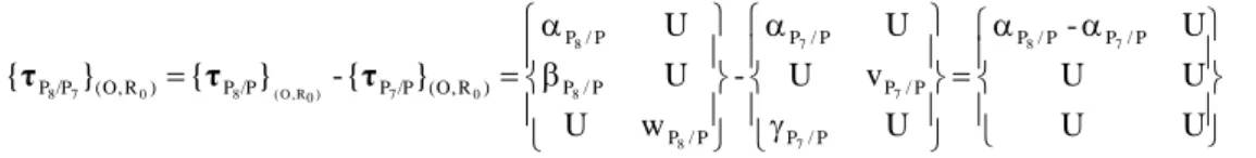
For the perpendicularity tolerance of surface P8 with reference to surface P7 (datum surface), this functional tolerance is described by torsor {τP8/P7}(O,R0). And the geometric constraint of the perpendicularity tolerance also
depends only on rotation variations. It needs to check that all points of surface P8 are located in the spatial region between two parallel planes spaced with Tpe which are perpendicular to the specified datum plane. According to the analysis above, we have:
30 P 7 P 7 P 30 P 8 30 P 8 30 P P 30 P 30 P 7 30 P 7 30 P 30 P 8 P 8 P P 30 P 30 P 7 P 7 30 P 8 P 8 30 P 30 P ) (O,R /P P ) (O,R /P P ) (O,R /P P 7 8 8 8 7 7 7 7 8 8 7 8 7 8 0 7 0 8 0 7 8 α b U a U α b β a w U β α c β a w α c U a U U β β b U c β c U b α α } { -} { } {τ τ τ
Thus, we can obtain the following inequality to satisfy the perpendicularity tolerance requirement using relation (28): 0.02 ) α (α 60 30P 30 P8 7
6. Conclusions
In the context of integrated design and manufacturing, we focus our research on 3D modeling of manufacturing variations. The proposed model regards each machining set-up of the part as a mechanism, the SDT parameters are employed to represent the geometrical variations of the part caused by the positioning errors and machining operations during the successive machining set-ups and the SDT chains are used to model the deviation propagation between different set-ups. After having obtained all SDT chains according to the process planning of part, we can evaluate the effect of these variations on the part and check whether functional tolerances are respected, or determine the manufacturing tolerances according to the functional tolerances. An example has been presented to illustrate the application of the method in the field of CNC milling. Our future research works will focus on: the mathematical modeling of the machining-induced variation accumulation and propagation, and the development of methods and tools for manufacturing tolerance analysis and synthesis in multi-stage manufacturing process.
Acknowledgments
The authors would like to acknowledge the financial supports by the National Natural Science Foundation of China (Grant Nos. 52075222 and 51575235).
References
Abellán-Nebot, J. V., Subirón, F. R., and Mira, J. S., Manufacturing variation models in multi-station machining systems, International Journal of Advanced Manufacturing Technology, Vol. 64, No. 1-4, (2013), pp. 63-83.
Anselmetti, B., and Louati, H., Generation of manufacturing tolerancing with ISO standards, International Journal of Machine Tools and Manufacture, Vol. 45, No. 10 (2005), pp. 1124-1134.
Advanced Manufacturing Technology, Vol.61, No. 9-12, (2012), pp. 1085-1099.
Ayadi, B., Anselmetti, B., Bouaziz, Z., and Zghal, A., Three-dimensional modelling of manufacturing tolerancing using the ascendant approach, International Journal of Advanced Manufacturing Technology, Vol. 39, No. 3-4, (2008), pp. 279-290.
Bourdet, P., and Ballot, É., Geometrical behavior laws for computer aided tolerancing, In Proceedings of 4th CIRP Seminar on Computer Aided Tolerancing: April 1995, University of Tokyo, (1995), pp. 143-154.
Ji, P., A tree approach for tolerance charting, International Journal of Production Research, Vol. 31, No. 5(1993), pp. 1023-1033. Laifa, M., Sai, W. B., Hbaieb, M., Evaluation of machining process by integrating manufacturing dispersions, functional constraints,
and the concept of small displacement torsors, International Journal of Advanced Manufacturing Technology, Vol. 71, No. 5-8, (2014), pp. 1327-1336.
Legoff, O., Villeneuve, F., and Bourdet, P., Geometrical tolerancing in process planning: a tridimensional approach, Proceedings of the Institution of Mechanical Engineers Part B Journal of Engineering Manufacture, Vol. 213, (1999), pp. 635-640.
Legoff, O., Tichadou, S., and Hascoet, J. Y., Manufacturing errors modelling: two three-dimensional approaches, Proceedings of the Institution of Mechanical Engineers Part B Journal of Engineering Manufacture, Vol. 218, No. 12 (2004), pp. 1869-1873. Louati, J., Ayadi, B., Bouaziz, Z., and Haddar, M., Three-dimensional modelling of geometric defaults to optimize a manufactured
part setting, International Journal of Advanced Manufacturing Technology, Vol. 29, No. 3-4 (2006), pp. 342-348.
Nejad, M. K., Vignat, F., and Villeneuve, F., Simulation of the geometrical defects of manufacturing, International Journal of Advanced Manufacturing Technology, Vol. 45, No. 7-8 (2009), pp. 631-648.
Nejad, M. K., Vignat, F., and Villeneuve, F., Tolerance analysis in machining using the model of manufactured part (MMP) - comparison and evaluation of three different approaches, International Journal of Computer Integrated Manufacturing, Vol. 25, No. 2 (2012), pp. 136-149.
Ngoi, B. K. A., and Tan, C. S., Graphical approach to tolerance charting—a maze chart method, International Journal of Advanced Manufacturing Technology, Vol. 13, No. 4 (1997), pp. 282-289.
Peng, H., and Lu, W., Modeling of Geometric Variations within Three-dimensional Tolerance Zones, Journal of Harbin Institute of Technology (New Series), Vol. 25, No. 2 (2018), pp. 41-49.
Qin, Y., Lu, W., Qi, Q., Liu, X., Huang, M., Scott, P. and Jiang, X., Towards an ontology-supported case-based reasoning approach for computer-aided tolerance specification, Knowledge-Based Systems, Vol. 141, No. 2 (2018), pp.129-147.
Royer, M., and Anselmetti, B., 3D manufacturing tolerancing with probing of a local work coordinate system, International Journal of Advanced Manufacturing Technology, Vol. 84, No. 9-12 ( 2016), pp. 2151-2165.
Teissandier, D., Couétard, Y., and Gérard, A., A computer aided tolerancing model: proportioned assembly clearance volume, Computer-Aided Design, Vol. 31, No. 13 (1999), pp. 805-817.
Thimm, G., Wang, R., and Ma, Y., Tolerance transfer in sheet metal forming, International Journal of Production Research, Vol. 45, No. 14-15 (2007), pp. 3289-3309.
Vignat, F., Villeneuve, F., 3D transfer of tolerances using a SDT approach: application to turning process, Journal of Computing and Information Science in Engineering, Vol. 3, (2003), pp. 45-53.
Villeneuve, F., Legoff, O., and Landon, Y., Tolerancing for manufacturing: a three-dimensional model, International Journal of Production Research, Vol. 39, No. 8 (2001), pp. 1625-1648.
Villeneuve, F., and Vignat, F., 3D synthesis of manufacturing tolerances using a SDT approach, The 8th CIRP International Seminar on Computer Aided Tolerancing, Charlotte, North Carolina, Vol. 41, No. 3 (2003), pp. 279-290
Villeneuve, F., and Vignat, F., Manufacturing process simulation for tolerance analysis and synthesis, In: Bramley, A., Brissaud, D., et al. (eds) Advances in integrated design and manufacturing in mechanical engineering, Springer Netherlands, (2005), pp. 189-200.
Wang, R., Thimm, G., and Ma, Y., Review: geometric and dimensional tolerance modeling for sheet metal forming and integration with CAPP, International Journal of Advanced Manufacturing Technology, Vol. 51, No. 9-12 (2010), pp. 871-889.
Xue, J., and Ji, P., Process tolerance allocation in angular tolerance charting, International Journal of Production Research, Vol. 42, No. 18 (2004), pp. 3929-3945.
Zhang, J., and Qiao, L., Three dimensional manufacturing tolerance design using convex sets, Procedia CIRP, No.10 (2013), pp. 259-266.
Zhong, Y., Qin, Y., Huang, M., Lu, W., Gao, W., Du, Y., Automatically generating assembly tolerance types with an ontology-based approach, Computer-Aided Design, Vol. 45, No. 11 (2013), pp. 1253-1275.