UNCONDITIONAL EXISTENCE OF DENSITIES FOR THE NAVIER-STOKES EQUATIONS WITH NOISE (Mathematical Analysis of Viscous Incompressible Fluid)

UNCONDITIONAL EXISTENCE OF DENSITIES FOR THE NAVIER-STOKES

EQUATIONS WITH NOISE

MARCO ROMITO

ABSTRACT. Thefirst partof thepapercontainsashortreviewof recent results about the existence of densities for finite dimensional functionals of weak solutions of the

Navier-Stokes equationsforcedbyGaussian noise. Such resultsareobtained for solutionslimit

of spectral Galerkin approximations.

In the secondpart of the paper weprove via a ”transfer principl$e’$ thatexistence

of densitiesisuniversal, inthesensethat itdoesnotdepend onhow thesolutionhas

been obtained, given someminimal and reasonable conditions of consistence under conditional probabilities and weak-strong uniqueness. Aquantitative version of the transferprincipleisalso availablefor stationarysolutions.

1. INTRODUCTION

Whendealingwithastochastic evolutionPDE,the solutiondependsnotonly

on

the time andspace independentvariables, but alsoon th$e^{}$ chanc$e’$ variable, whichplays

a completely different role. The existence ofa density for the probability distribution of the solution is thusaform ofregularitywithrespecttothis newvariable.

In this paper we detail some results related to the existence of densities of finite dimensional projectionsof

any

solutionof theNavier-Stokes equations

$\dot{u}+(u\cdot\nabla)u+\nabla p=v\Delta u+\eta,$

(1.1)

divu $=0,$

withDirichletboundaryconditionsonabounded domain,orwithperiodic boundary conditionsonthe torus. Here$\eta$isGaussiannoise. Most ofthe results haveappearedin

[DR14, Rom13],

_some

_{additional results}arein

progress

$[Roml4b, Roml4c, Roml4a].$ To be more precise,

our

result

concerns

the existence of densities for finite dimen-sional functionals ofthe solution, and one reason for this is that there is no canonical reference

measure

in infinite dimension, as is the Lebesgue

measure

in finite dimen-sion. Tounderstandtheright referencemeasureisanopenproblemevenindimension

twoandfor

any

suitable choice of thedrivingnoise.

Our interest in the existence of densities stems from a series of mathematical

mo-tivations. The first and foremost is the investigation of the regularity properties of solutionsofthe Navier-Stokes equations.

On the other hand regularityis notthe only

open

problem inthemathematical

the-oryoftheNavier-Stokes equations (eitherwithrandomforcing,orwithout). The first obvious choice is the relatedproblemofuniqueness. Intheprobabilistic frameworkwe candealwith differentnotions ofuniqueness, the weakerbeingthe statistical

unique-ness,that is_{the uniqueness of distributions. Although}the results detailedinthis

paper

2010MathematicsSubject_{Classification.} Primary$76M35,\cdot$Secondary$60H15,$ $60G30,$ $35Q30.$

Keywordsandphrases. Densityoflaws,Navier-Stokesequations,stochasticpartial differential

are

very

far from

any

uniqueness result,

we

mention that the law of

an

infinite

di-mensional randomvariable

can

be characterized bythe laws ofits finite dimensional

projections. By the results of [FR08], itis then sufficient to show that the laws oftwo solutions

agree

at

every

time. Aneveneasiercondition, _following from the resultsof [Rom08], requiresthatwe show agreementbetweenthelaws ofthe corresponding in-variantmeasures,thatis,ifthe

processes agree

attime$t=\infty$,thenthey

agree

forevery

time,includingtheir time correlations.

An additional $($rather

vague

though$)^{}$ folkloristi$c’$ motivation for the interest in

fi-nite dimensional projections is that most of the real-life experiments to evaluate the velocityofa fluidarebased on a finite number ofsamples inafinite numberof points

(Eulerianpointofview),orby tracing

some

particles(smoke,etc$\cdots$) moving according

to the fluid velocity (Lagrangian point ofview). The literature on experimental fluid

dynamics is huge. Here werefer for instance to [Tav05] for

some

examples ofdesign

of

experiments.

Let

us

focus

on

the Eulerian

point

of view. To

simplify,

consider

a

torus, then sampling the velocity field means measuring the velocity in

some

space

points$y_{1}$,.. . ,$v_{d}:urightarrow(u(t,y_{1}), \ldots,u(t_{Vd}))$,andabitofFourier seriesmanipulations

showsthat this is$a”projection”.$

Aninteresting difficultyinproving regularityof thedensity

emerges

asa by-product of the(more_{general and}fundamental!) _{problem of proving uniqueness and}regularity

ofsolutions of the Navier-Stokesequations. Indeed, afundamental and classical tool isthe Malliavincalculus,adifferential calculus where the differentiating variableisthe underlyingnoise driving the system. The Malliavin derivative $\mathcal{D}_{H}u(t)$, the derivative

withrespecttothevariations of the noiseperturbation, isgivenas

$\mathcal{D}_{H}u=\lim_{\epsilon\downarrow 0}\frac{u(W+\epsilon\int Hds)-u(W)}{\epsilon},$

where

we

have written the solution $u$

as

$u(W)$ to show the explicit dependence of $u$ from the noise forcing. We point, for instance, to [Nua06] for further details and definitions, and

we

onlynotice that the Malliavin derivative $\mathcal{D}_{H}u$ofthesolution$u$of (1.1),asavariation, satisfies thelinearizationaround thesolution,namely,

$\frac{d}{dt}\mathcal{D}_{H}u-v\Delta \mathcal{D}_{H}u+(u\cdot\nabla)\mathcal{D}_{H}u+((\mathcal{D}_{H}u)\cdot\nabla)u=SH,$

andgood estimates

on

$\mathcal{D}_{H}u(t)$originateonly from goodestimatesonthe linearization

of (1.1),which arenot availableso far. This settles the need ofmethods to

prove

exis-tenceandregularityof thedensitythat do not rely onthis calculus,as donein[DR14].

In this

paper

wetackle theproblem ofuniversalityofthe resultobtained in[DR14],

which

are

valid only for limits of Galerkin approximations. At the present time we

do not know ifthe Navier-Stokes equations admit a unique $distribution_{r}$therefore it might happen that solutions obtained by differentmeans

may

have different

proper-ties. Inawaythis isreminiscentoftheproblem ofsuitableweaksolutions introduced by[Sch77]. Onlymuch laterithasbeenprovedthat solutions obtained bythe spectral Galerkin methods are suitable [Gue06] (under

some

$non\dashv$rivial conditions though), andhence results ofpartial regularity aretrue forthose solutions.

Ourmaintheorem is$a^{ノ/}$transfer principl$e’$ (Theorem 4.1), thatstates that

as

long

as

we can

prove

existence of adensity for afinite dimensional functionalofthe solution andforaweaksolution that satisfies weak strong uniqueness,then existenceofa density

holdsfor

any

other solutionsatisfying weak-strong uniquenessandaclosureproperty

withrespectto conditional probabilities.

Animportant limitationofourtransferprincipleis that itappliesonlyon’

instanta-neou$s’$ properties, namelyto randomvariablesdepending onlyon onetime,in

partic-ular,theresultson timecontinuityofdensities in $[Roml4c]$ arestill outof reach.

The transfer principleisqualitativeinnature,asit

may

transferonlythe existence. In

general

no

quantitative information

can

beinherited. This

seems

tobemainly

an

arte-fact of the proof,that in turns dependson good momentsofthe solution in smoother

spaces. Indeed, inthecaseofstationarysolutions,

_we

canprove a quantitativeversion ofthe principle(Theorem 4.2).

2. WEAKSOLUTIONS

We consider problem (1.1) with either periodic boundary conditions on the three-dimensional torus $\mathbb{T}_{3}=[0,$ $2\pi|^{3}$orDirichletboundaryconditionsonasmooth domain

$0\subset R^{3}$. We will understand weakmartingalesolutions of_(1.1)

as

probability

measures

on the path space. We will then define legit families of solutions as classes of solu-tionsthatareclosed by conditional probabilityandfor which weak-strong uniqueness holds.

2.1. Preliminaries. Let $H$ be the standard

space

of

square

summable divergence free

vectorfields, defined as the closure ofdivergence free smooth vector fields satisfying

theboundary condition, with innerproduct $\rangle_{H}$ and norm $\Vert$ $\Vert_{H}$. Define likewise V as the closure with respect to the $H^{1}$ norm. Let $\Pi_{L}$ be the Leray projector, $A=$

$-\Pi_{L}\Delta$the Stokes operator,and denoteby $(\lambda_{k})_{1c\geq 1}$ and $(e_{k})_{k\geq 1}$ the eigenvaluesandthe

correspondingorthonormal basis of eigenvectors of A. Define the bi-linear operator

$B$ : _{$V\cross Varrow V’$} as _{$B(u,\nu)=\Pi_{L}(u\cdot\nabla\nu)$},

$u,\nu\in$ V. We recall that $\langle u_{1},$$B(u_{2},u_{3})\rangle=$

$-\langle u_{3},$$B(u_{2},u_{1}$ We refer to Temam [Tem95] for a detailed account of all the above definitions.

The noise$\dot{\eta}=S\dot{W}$in(1.1)iscoloured inspaceby a

covarianceoperatorS$\star$

@ $\in \mathscr{L}$(H),

where$W$isa cylindrical Wiener

process

_{(see [DPZ92] forfurther details). We}

assume

that @$\star$

@ is trace-class and

we

denote by $\sigma^{2}=R(@^{\star}@)$ its trace. Finally, consider the

sequence

$(\sigma_{k}^{2})_{k\geq 1}$ of eigenvaluesof@ $\star$

@,and let $(q_{k})_{k\geq 1}$ be the orthonormal basis in $H$

of eigenvectors of@$\star$

S. Forsimplicity we may assume thatthe Stokes operator A and the covariance commute,sothat

$\dot{\eta}(t,y)=SdW=\sum_{k\in Z_{\star}^{3}}\sigma_{k}\dot{\beta}_{k}(t)e_{k}(v)$.

2.2. Weak and strong solutions. With the abovenotations,

_{we can}

recastproblem(1.1)

as an

abstractstochasticequation,

(2.1) _{$du+(vAu+B(u))dt=SdW,$}

with initial condition $u(0)=x\in$ H. It is well-known [Fla08] that for

every

$x\in H$

there exist a martingale solution of this equation, that is a filtered probability

space

$(\tilde{\Omega},\overline{\mathscr{F},}\tilde{\mathbb{P}},\{\overline{\mathscr{F}_{t}}\}_{t\geq 0})$

,_{a cylindrical}Wiener

process

$\overline{W}$

anda

process

$u$withtrajectories in $C([0, \infty);D(A)’)\cap L_{1oc}^{\infty}([0, \infty), H)\cap L_{1oc}^{2}([0, \infty);V)$ adapted_to$(\overline{\mathscr{F}_{t}})_{t\geq 0}$

such thatthe above equationis satisfied with$\overline{W}$

replacing$W.$

Wewilldescribe,equivalently,a martingale solutionas ameasure onthepathspace

be its Borel $\sigma$

-algebra.

Denoteby $\mathscr{F}_{t}^{NS}$ the $\sigma$-algebra

generated

by the restrictions of

elements of $\Omega_{NS}$ to the interval $[0, t]$ (roughly speaking, this is the

same

as

the Borel

$\sigma$-algebraof $C([0, t];D(A)’)$). Let$\xi$be thecanonical

process,

definedby$\xi_{t}(\omega)=\omega(t)$,

for $\omega\in\Omega_{NS}$

Definition2.1([FR08]). Aprobability measure$\mathbb{P}$

on

$\Omega_{NS}$isasolution of themartingale

problemassociatedto (2.1)with initial distribution $\mu$if

$\blacksquare \mathbb{P}[L_{1\circ c}^{\infty}(R^{+}, H)\cap L_{1oc}^{2}(R^{+};V)]=1,$

$\blacksquare$ foreach$\phi\in D(A)$, the

process

$\langle\xi_{t}-\xi_{0}, \phi\rangle+\int_{0}^{t}\langle\xi_{s}, A\phi\rangle-\langle B(\xi_{s}, \phi) , \xi_{s}\rangle ds$

is

a

continuous

square

summable martingale with quadratic variation $t\Vert S\phi\Vert_{H}^{2}$

(henceaBrownianmotion),

$\blacksquare$ the

marginalof$\mathbb{P}$

attime $0$is $\mu.$

The second condition in the definition above has a twofold meaning. On the one

hand it states that the canonical

process

is aweak (intermsof PDEs) solution,

on

the otherhand it identifies the driving Wiener

process,

and hence is a weak (in terms of stochasticanalysis) solution.

2.2.1. Strongsolutions. It is also well-known that (2.1) admits local smooth solutions defined

up

toarandom time(a_stoppingtime,infact)$\tau_{\infty}$ that correspondstothe

(pos-sible)timeofblow-upinhigher

norms.

To consideraquantitativeversion of the local smoothsolutions,_noticethat$\tau_{\infty}$

can

beapproximated monotonicallybya

sequence

of

stoppingtimes

$\tau_{R}=\inf\{t>0:\Vert Au_{R}(t)\Vert_{H}\geq R\},$

where$u_{R}$ isasolution of the following problem,

$du_{R}+(vAu_{R}+\chi(\Vert Au_{R}\Vert_{H}^{2}/R^{2})B(u_{R},u_{R}))dt=@dW,$

with initial condition in$D(A)$, andwhere$\chi$ : $[0, \infty$) $arrow[0$, 1$]$ is a suitable $cut-0ff$

func-tion, namely a non-increasing $C^{\infty}$ function such that_{$\chi\equiv 1$}

on

$[0$, 1$]$ and _{$\chi_{R}\equiv 0$}

on

[2,$\infty)$

.

The

process

_{$u_{R}$} is a strong (in PDE sense) solution of the cut-off equation.

Moreover it isa strong solution alsointermsof stochastic analysis,

so

itcanberealized uniquelyon

any

probability

space,

giventhe noiseperturbation.

As it iswell-known in thetheory ofNavier-Stokesequations,theregularsolution is unique in the class of weaksolutions that satisfy

some

formof the

energy

inequality.

We willgivetwoexamplesofsuch classes for the equations withnoise.

Remark 2.2. The analysis of strong (PDE meaning) solutions can be done on larger

spaces, up

to $D(A^{1/4})$,which is acritical

space

with respectto the Navier-Stokes

2.2.2. Solutionssatisfyingthe almostsure

energy

inequality. Analmostsureversionof the

energyinequalityhas beenintroduced in [Rom08, RomlO]. _Given aweak solution $\mathbb{P},$

choose $\phi=e_{k}$

as

atest functioninthe second propertyof Definition 2.1, to get aone

dimensional standard Brownian motion $\beta^{k}$. Since $(e_{k})_{k\geq 1}$ isanorthonormalbasis,the

$(\beta^{k})_{k\geq 1}$ are a

sequence

ofindependentstandardBrownian motions. Then the

process

$W_{\mathbb{P}}= \sum_{k}\beta^{k}e_{k}$ is a cylindrical Wiener

process1

on

H. Let $z_{\mathbb{P}}$ be the solution to the

linearization at$0$ of (2.1),namely $dz_{\mathbb{P}}+Az_{\mathbb{P}}=SdW_{\mathbb{P}}$, with initial condition$z(0)=0.$

Finally,set$\nu_{\mathbb{P}}=\xi-z_{\mathbb{P}}$. It turns out that$\nu_{\mathbb{P}}$ isasolution of

$\dot{\nu}+vA\nu+B(\nu+z_{\mathbb{P}},\nu+z_{\mathbb{P}})=0, \mathbb{P}-a.s.,$

with initial condition$\nu(0)=\xi_{0}$. An

energy

balancefunctional

can

beassociated to$\nu_{\mathbb{P}},$ $\mathcal{E}_{t}(\nu, z)=\frac{1}{2}\Vert\nu(t)\Vert_{H}^{2}+v\int_{0}^{t}\Vert\nu(r)\Vert_{V}^{2}dr-\int_{0}^{t}\langle z(r)$,$B(\nu(r)+z(r),\nu(r))\rangle_{H}$ dr.

We saythatasolution$\mathbb{P}$

ofthemartingaleproblemassociated to (2.1) (asinDefinition 2.1)satisfiesthealmostsure

energy

inequalityifthere isaset$T_{P}\subset(0, \infty)$ ofnullLebesgue

measure

such that forall$s\not\in T_{P}$ and all$t\geq s,$

$P[\mathcal{E}_{t}(\nu, z)\leq \mathcal{E}_{s}(\nu, z)]=1.$

Itis not difficulttocheck that $\mathcal{E}$

is measurable and finite almostsurely.

2.2.3. A martingale version

_of

the energy inequality. An alternative formulation of the

energy

inequality that, on the one hand is compatible with conditional probabilities,

and onthe other handdoesnotinvolveadditional quantities (such

as

the

processes

$z_{\mathbb{P}}$

and$\nu_{\mathbb{P}})$ canbe givenin terms of super-martingales. The additional advantage is that

thisdefinition is keentogeneralizationtostate-dependentnoise.

Define,for

every

$\mathfrak{n}\geq 1$, the

process

$\mathscr{E}_{\iota^{1}}=\Vert\xi_{t}\Vert_{H}^{2}+2v\int_{0}^{t}\Vert\xi_{s}\Vert_{V}^{2}$ds-2Tr(@

$\star$

S),

and,moregenerally, forevery$\mathfrak{n}\geq 1,$

$\mathscr{E}_{t}^{\mathfrak{n}}=\Vert\xi_{t}\Vert_{H}^{2\mathfrak{n}}+2\mathfrak{n}v\int_{0}^{t}\Vert\xi_{s}\Vert_{H}^{2\mathfrak{n}-2}\Vert\xi_{s}\Vert_{V}^{2}ds-\mathfrak{n}(2\mathfrak{n}-1)R(S^{\star}S)\int_{0}^{t}\Vert\xi_{s}\Vert_{H}^{2\mathfrak{n}-2}$ds,

when $\xi\in L_{1oc}^{\infty}([0, \infty);H)\cap L_{1\circ c}^{2}([0, \infty);V)$, and$\infty$ elsewhere.

We

say

thatasolution$\mathbb{P}$

ofthemartingaleproblem associatedto(2.1) (asinDefinition 2.1) satisfies the super-martingale

energy

inequality if for each $\mathfrak{n}\geq 1$, the

process

$\mathscr{E}_{t}^{\mathfrak{n}}$

defined above is $\mathbb{P}$

-integrable and for almost every $s\geq 0$ (including $s=0$) and all

$t\geq s,$

$\mathbb{E}[\mathscr{E}_{\iota^{\mathfrak{n}}}|\mathscr{F}_{s}^{NS}]\leq \mathscr{E}_{s}^{\mathfrak{n}},$

or,in otherwords,ifeach$\mathscr{E}^{\mathfrak{n}}$

is an almostsure supermartingale. $1_{Notice}$_that$W$is measurable withrespect_{tothesolution}process.

2.3.

Legit families of weak solutions.

Following

the

spirit

of [FR08], given $x\in H,$

denote by $\mathscr{C}(x)$

any

familyof non-emptysets ofprobability

measures on

$(\Omega_{NS}, \mathscr{F}^{NS})$

that are solutions of (1.1) with initial condition$x$, as specified by Definition 2.1, and

suchthatthefollowing propertieshold,

$\blacksquare$ the sets _{$(\mathscr{C}(x))_{x\in H}$}

are

closeunder

conditioning, namely for

every

$\mathbb{P}\in \mathscr{C}(x)$ and

every

$t>0$, if $(\mathbb{P}|_{\mathscr{F}_{t}^{NS}}^{\omega})_{\omega\in\Omega_{NS}}$ isthe regular conditionalprobabilitydistribution of

$\mathbb{P}$

given$\mathscr{F}_{t}^{NS}$, then$\mathbb{P}|_{\mathscr{T}_{t}^{NS}}^{\omega}\in \mathscr{C}(\omega(t))$,for$\mathbb{P}-a.e.$ $\omega\in\Omega_{NS},$

$\blacksquare$ weak-strong uniquenessholds,namelyfor

every

$x\in D(A)$ and

every

$\mathbb{P}\in \mathscr{C}(x)$,

$\xi(t)=u_{R}(t,x)$for

every

$t<\tau_{R},$$\mathbb{P}-a.s$,where

$u_{R}$ x) isthe local smoothsolution

withinitial condition$x.$

Wewill call eachfamily $(\mathscr{C}(x))_{x\in H}$ satisfyingthetwo aboveproperty a legit family.

It isclear that the classes definedin [FR08] (detailedin section2.2.3) andin[Rom08, RomlO] (detailed in section 2.2.2) are of this kind,

as

they actually satisfy the

more

restrictive condition called reconstruction in the above-mentioned

papers.2

It is also straightforward that the $x$-wise set union of two legit families is again

a

legit

fam-ily. A less obvious fact is that the family of sets of solutions obtained as limits of Galerkin approximations is legit. This is remarkable

as

limits of Galerkin

approxi-mations do not satisfy the reconstruction property. To

see

this fact,

we

first observe that limit of Galerkin

approximatio\’{n}

satisfy the

energy

inequality, and hence fall in thesameclass definedin [Rom08, RomlO]. Inparticular, dueto the

energy

inequality,

weak-strong uniquenessholds. Moreover,

_once

thesub-sequenceof Galerkin

approx-imations is identified, the regular conditional probability distributions of the

approx-imations,_along the sub-sequence,

converge

to the correspondingregular conditional

probabilitydistributions of thelimit(uniquelyidentifiedbythe sub-sequence). 3. EXISTENCE OF DENSITIES

In this section we givea short review of the results contained in the

papers

[DR14,

$Roml4c,$ $Roml4a]$ (see also [Rom13]). To this end we recall the definition of Besov

spaces.

The general definitionisbased onthe Littlewood-Paleydecomposition,but it is notthe best suited forour

purposes.

Weshall

use

analtemativeequivalentdefinition

(see [Tri83, Tri92]) in terms of differences. Define

$(\Delta_{b}^{1}f)(x)=f(x+b)-f(x)$_,

$( \Delta_{b}^{\mathfrak{n}}f)(x)=\Delta_{b}^{1}(\Delta_{h}^{\mathfrak{n}-1}f)(x)=\sum_{\mathfrak{j}=0}^{\mathfrak{n}}(-1)^{\mathfrak{n}-j}(\begin{array}{l}\mathfrak{n}\mathfrak{j}\end{array})f(x+\mathfrak{j}b)$,

then the followingnorms, for $s>0,$ $1\leq p\leq\infty,$ $1\leq q<\infty\backslash$,

$\Vert f\Vert_{B_{p,q}^{s}}=\Vert f\Vert_{Lp}+(\int_{\{|b|\leq 1\}}\frac{\Vert\Delta_{b}^{\mathfrak{n}}f||_{L}^{q_{p}}}{|b|^{sq}}\frac{dh}{|h|^{d}})^{\frac{1}{q}}$

and for $q=\infty,$

$\Vert f\Vert_{B_{p,\infty}^{s}}=\Vert f\Vert_{Lp}+\sup_{|b|\leq 1}\frac{\Vert\Delta_{b}^{\mathfrak{n}}f\Vert_{Lp}}{|h|^{\alpha}},$

$2_{Reconstruction}$_{, roughlyspeaking, requires that ifonehas a} $\mathscr{F}_{t}^{NS}$ measurable map$x\mapsto \mathbb{Q}_{x/}$ with

$\mathbb{Q}_{x}\in \mathscr{C}(x)$,and$\mathbb{P}\in \mathscr{C}(x_{0})$,thentheprobability measure given by$\mathbb{P}$on

$[0, t]$, and,conditionaly on$\omega(t)$, by the values of$\mathbb{Q}$.,isanelement of$\mathscr{C}(x_{0})$.

where$\mathfrak{n}$is

any

integersuch that_{$s<\mathfrak{n}$},are

equivalentnormsof$B_{p,q}^{s}(R^{d})$ for thegiven

range

ofparameters.

Thetechniqueintroduced in[DR14] is basedontwo ideas. The first is thefollowing

analytic lemma, which provides a quantitative integration by parts. The lemma is

implicitlygivenin [DR14] andexplicitlystated andproved in $[Roml4c].$

Lemma 3.1 (smoothing lemma).

_If

$\mu$ is a

finite

measure

on

$R^{d}$ and there are an integer $m\geq 1$, tworeal numbers _$s>0,$ $\alpha\in(0,1)$, with_$\alpha<s<m$, andaconstant$c_{1}>0$ such that

for

every

$\phi\in C_{b}^{\alpha}(R^{d})$ and$b\in R^{d},$

$| \int_{R^{d}}\Delta_{h}^{m}\phi(x)\mu(dx)|\leq c_{1}|b|^{S}\Vert\phi\Vert_{C_{b}^{\alpha}},$

then $\mu$has a density$f_{\mu}$ with respect to the Lebesgue

measure on

$R^{d}$ and$f_{\mu}\in B_{1,\infty}^{r}$

for

every

$r<s-\alpha$. Moreover,thereis $c_{2}=c_{2}(r)$ such that

$\Vert f_{\mu}\Vert_{B_{1,\infty}^{r}}\leq c_{2}c_{1}.$

The secondidea is to use the random perturbationtoperform th$e^{}$ fractiona$l’$

inte-gration byparts alongthe noise to be used inthe above lemma. Thebulkof this idea

can be found in [FP10]. Our method is based

on

the

one

hand

on

the idea that the Navier-Stokesdynamicsi$s^{}$

goo

$d’$ for shorttimes, and onthe other hand that

Gauss-ian

processes

have smooth densities. When tryingto estimate the Besov norm ofthe density,weapproximatethe solutionby splittingthe timeinterval in twoparts,

time

Onthe firstparttheapproximatesolution$u_{\epsilon}$is the

same

astheoriginalsolution,onthe

second part thenon-linearity is killed. By Gaussianity this is enough to estimate the increments of thedensity of$u_{e}$

.

Since $u_{\epsilon}$ is the one-step explicitEulerapproximation

of$u$, the errorinreplacing$u$by $u_{\epsilon}$

can

beestimated in terms of $e$. Byoptimizing the

increment

versus

$e$

we

haveanestimate

on

the derivativesof the density.

The final result is given in the proposition below. Incomparisonwith Theorem 5.1 of [DR14],_{herewe give an explicit dependenceof the Besov normof the density}with respecttotime. The estimatelooksnotoptimal though.

The regularityof the density can beslightly improvedfrom $B_{1,\infty}^{1-}$ to $B_{1,\infty}^{2-}$ if$u$ is the stationarysolution,_namelythe solution whose statisticsare independentfrom time. Proposition 3.2. Given $x\in H$ _and a

finite

dimensional subspace $F$

of

$D(A)$ generated by

the eigenvectors

_of

$A$_, namely $F=span[e_{\mathfrak{n}_{1}}, \cdots, e_{\mathfrak{n}_{F}}]$

for

some arbitrary indices $\mathfrak{n}_{1}$,

$\cdots$ ,$\mathfrak{n}_{F},$

assume that $\pi_{F}S$ is invertible on F.

Thenfor

every$t>0$ theprojection $\pi_{F}u(t)$ has an almost everywhere positive density $f_{F,t}$ with respect to the Lebesgue measure on $F$, where _$u$ is any

solution

_of

(2.1) whichis limitpoint

_of

thespectral Galerkin approximations.

Moreover,

_for

_every

$\alpha\in(0,1)$, $f_{F,t}\in B_{1,\infty}^{\alpha}(R^{d})$ and

for

every

small $e>0$, there exists

$c_{3}=c_{3}(e)>0$suchthat

$\Vert f_{F,t}\Vert_{B_{1,\infty}^{\alpha}}\leq\frac{c_{3}}{(1\wedge t)^{\alpha+e}}(1+\Vert x\Vert_{H}^{2})$.

Proof.

Given a finite dimensional space $F$ as in the statement of the proposition, fix

cases.

$If|b|^{2\mathfrak{n}/(2\alpha+\mathfrak{n})}<t$, then

we

usethe

same

estimatein[DR14] toget

$|\mathbb{E}[\Delta_{\dagger\iota}^{m}\phi(\pi_{F}u(t))]|\leq c_{4}(1+\Vert x\Vert_{H}^{2\alpha})\Vert\phi\Vert_{C_{b}^{\alpha}}|b|^{\frac{2\mathfrak{n}\alpha}{2\infty+\mathfrak{n}}}.$

Ifonthe other hand $t\leq|b|^{2\mathfrak{n}/(2\infty+\mathfrak{n})}$, we introduce the

process

$u_{\epsilon}$ as above, butwith

$\epsilon=t$. As in [DR14],

$\mathbb{E}[\Delta_{h}^{m}\phi(\pi_{F}u(t))]=\mathbb{E}[\Delta_{h}^{m}\phi(\pi_{F}u_{\epsilon}(t))]+\mathbb{E}[\Delta_{b}^{m}\phi(\pi_{F}u(t))-\Delta_{b}^{m}\phi(\pi_{F}u_{\epsilon}(t))]$

and

$|\mathbb{E}[\Delta_{b}^{m}\phi(\pi_{F}u(t))-\Delta_{b}^{m}\phi(\pi_{F}u_{\epsilon}(t))]|\leq c_{5}(1+\Vert x\Vert_{H}^{2\propto})\Vert\phi\Vert_{C_{b}^{\alpha}}t^{\infty}.$

Forthe probabilistic error

we

usethe fact that$u_{\epsilon}(t)$ isGaussian,hence

$| \mathbb{E}[\Delta_{b}^{m}\phi(\pi_{F}u_{\epsilon}(t))]|\leq c_{6}\Vert\phi\Vert_{\infty}(\frac{|h|}{\sqrt{t}})^{\frac{2\mathfrak{n}\alpha}{2\alpha+\mathfrak{n}}}$

Inconclusion, frombothcases

we

finallyhave

$|\mathbb{E}[\Delta_{b}^{m}\phi(\pi_{F}u(t))]|\leq C_{7(1+\Vert x\Vert_{H}^{2})\Vert\phi\Vert_{C_{b}^{\alpha}}|b|^{\frac{2\mathfrak{n}\alpha}{2\alpha+\mathfrak{n}}(1\wedge t)^{-\frac{\mathfrak{n}\alpha}{2\infty+\mathfrak{n}}}}}.$

The choiceof$\mathfrak{n}$and $\alpha$yieldsthe final result.

$\square$

Remark 3.3. In [DR14]

we

introduced three different methods to

prove

existence of densities. The first method is based on the Markov machinery developed in [FR08] (see _also [DPD03]), whilethe thirdone is the one

on

Besov bounds detailedabove. $A$ secondpossibilityis to use anappropriateversionof theGirsanov changeofmeasure.

It tumsoutthat,together,theGirsanovchangeof

measure

and the Besov boundsyield

time regularityofthe densities of finitedimensional projections $[Roml4c].$

As it

may

be expected, the time regularity obtained is ”hal$f’$ the

space

regularity,

andthe densityis atmost $\frac{1}{2}$ H\"olderintimewith values in

$B_{1,\infty}^{\alpha}$,for$\alpha<1.$

Remark 3.4. An apparent drawback of the method is that it canonly handle finite di-mensional projections. There are interesting functions of the solution, the

energy

for

instance,that cannot be

seen

in

any way

asfinite dimensional projections. On the other

hand,

one can use

the

same

ideas(fractionalintegration by partsandsmoothingeffect

of thenoise) _directlyonsuchquantities.

Following this idea, in $[Roml4b]$ it is shown that the two quantities $\Vert u(t)\Vert_{H^{-s}}^{2}$ and $\int_{0}^{t}\Vert u(t)\Vert_{H^{1-s/}}^{2}$with $s<\frac{3}{4}$,haveadensity. Unfortunately, thereis a regularityissue that

preventsgettingdensities when$s\geq\frac{3}{4}$,unless $s=0$

.

Thespecialquantity

$\Vert u(t)\Vert_{H}^{2}+2v\int_{0}^{t}\Vert u(s)\Vert_{V}^{2}$ $ds$,

which representsthe

energy

balance and isquite relevant inthe theory, admitsa den-sity. Thisispossibledue to$tHe$fundamental cancellationpropertyof the Navier-Stokes

non-linearity.

Remark 3.5. An interesting question, thathas been completelyanswered for the two-dimensional

case

in [MP06],

concems

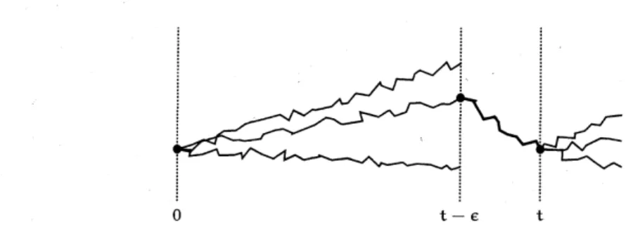
the existence of densities when the covariance of the drivingnoise is essentiallynon-invertible. The typical perturbation in(1.1) we consider here is

$0$ $t$ $\epsilon$ $t$

FIGURE 1. The strategy for the transfer principle:

we

only look at the smooth solutionimmediatelybeforethe evaluationtime.

where $\mathcal{Z}\neq Z_{\star}^{3}$ and is usually much smaller (finite, for instance). The idea is that the

noise influence is spread, by the non-linearity, to all Fourier components. The

con-ditionthat should ensure this has beenalreadywell understood [Rom04], and

corre-sponds to_{the fundamental algebraic property}that SCshouldgeneratethe whole

group

$Z^{3}.$

Itisclear thatthemethodwehave usedto obtain Besov bounds cannot work in this

case,because thenon-linearity plays a major role. Ontheother hand in $[Roml4a]$_we

prove,

using ideas similarto those leadingtothe transfer principle (Theorem 4.1),the existence ofa density No

regularity

properties

are

possible, though.

4. THETRANSFER PRINCIPLE

In this final section we present two results in the direction of extending results

provedonlyfora specialclass of solutions(limitsofspectralGalerkinapproximations in[DR14]) to

_every

legitsolution of (1.1). As alreadymentioned, the transferprinciple allows the extension ofinstantaneous properties, namely propertiesthat depend on a

singletime.

Given$t_{0}>0$,consider the followingevent in$\Omega_{NS},$

$L(t_{0})=$

{

$\omega$ : thereis $e>0$such that

$\sup_{t\in[t_{0}-e,t_{0}]}\Vert A\omega(t)\Vert_{H}<\infty$

}.

From$[Roml4b]$we_knowthat,if$(\mathscr{C}(x))_{x\in H}$ isa legitfamily,if_{$x\in H$}and$\mathbb{P}\in \mathscr{C}(x)$,then

$\mathbb{P}[L(t_{0})]=1$ for

a.e.

_{$t_{0}>0$}. To be

more

precise, theproofisgivenin$[Roml4b]$ only for

those legit families introduced in [FR08] and [RomlO], butthe two crucial properties used in the proof of the probability one statement are exactly those defining a legit family.

Our main theorem is given below. The intuitive idea is thatifwe are able to

prove

existence ofadensity (with_respecttoasuitableLebesguemeasure) forafinite dimen-sional functional ofa solution, then the

same

holds for

any

other solution, regardless

ofthe

way

we wereable toproduceit.

In other words, we

can prove

existence of a density for solutions obtained from Galerkin approximation, and this result will extend straight

away

toany other solu-tions,for instance thoseproduced bytheLerayregularization(seefor instance[Lio96]). Or

we

can use the special properties ofMarkov solutions given in [FR08, RomlO] to

prove

existence of densities ofa large class of finite dimensional functionals,

as

done inthe firstpart of[DR14],andagain this extends immediatelyto

any

(legit) solution.

Theorem 4.1 (Transfer principle). Let $d\geq 1$ and let $F$ : $D(A)arrow R^{d}$ be

a

measurable

junction. Assume thatwe are given alegitclass $(\mathscr{C}(x))_{x\in H}$andafamily $(\mathbb{Q}_{x})_{x\in H}$

of

solutions

of

(1.1)satisfying (only)weak stronguniqueness.

Iffor

every

$x\in D(A)$ and almost

every

$t_{0}>0$ the random variable $\omega\mapsto F(\omega(t_{0}))$

on

$(\Omega_{NS}, \mathscr{F}^{NS}, \mathbb{Q}_{X})$ has a density with respect to the Lebesgue measure

on

$R^{d}$, then

for

every

$x\in H$,

every

$\mathbb{P}\in \mathscr{C}(x)$ and almost

every

_{$t_{0}>0$}, the random variable $\omega\mapsto F(\omega(t_{0}))$ on

$(\Omega_{NS}, \mathscr{F}^{NS},\mathbb{P})$ hasadensitywithrespect totheLebesguemeasure on$R^{d}.$

Proof.

Following$[Roml4b]$,consider for

every

$e\leq 1$and

every

$R\geq 1$theevent$L_{\epsilon,R}(t_{0})$

defined

as

$L_{\epsilon,R}(t_{0})=\{\sup_{t\in[t_{0}-\epsilon,t_{0}]}\Vert A\omega(t)\Vert_{H}\leq R\}.$

Clearly $L(t_{0})=\cup L_{e,R}(t_{0})$

.

Given ameasurable function $F$

as

inthe standing

assump-tions, aLebesguenull set$E\subset R^{d}$,astate _{$x\in H$}andasolution$\mathbb{P}\in \mathscr{C}(x)$,

$\mathbb{P}[F(\omega(t_{0}))\in E]=\sup_{e\leq 1,R\geq 1}\mathbb{P}[\{F(\omega(t_{0}))\in E\}\cap L_{e,R}(t_{0})].$

Given $e\leq 1$ and $R\geq 1$,

we

condition $\mathbb{P}$

at time $t_{0}-e$ and we know that $\mathbb{P}|_{\mathscr{F}_{t}^{NS}}^{\omega}.$ $\in$

$\mathscr{F}_{t_{0}-\epsilon}^{NS}.$ Hence,usingw

$e^{0}ak^{\epsilon}-$

strongu

$niqueness\mathscr{C}(\omega(t_{0}-\epsilon)),$where$\mathbb{P}|_{\mathscr{F}_{t}^{N}}^{\omega}\underline{s}istheregu1arc$onditionalprobabilitydistributionof

$\mathbb{P}$

given

$\mathbb{P}[\{F(\omega(t_{0}))\in E\}\cap L_{\epsilon,R}(t_{0})]=\mathbb{E}^{\mathbb{P}}[\mathbb{P}[\{F(\omega(t_{0}))\in E\}\cap L_{\epsilon,R}(t_{0})|\mathscr{F}_{t_{0}-\in}^{NS}]]$

$=\mathbb{E}^{\mathbb{P}}[\mathbb{P}|_{\mathscr{F}_{t_{0}\epsilon}^{N\underline{S}}}^{\omega}[F(\omega’(e))\in E, \tau_{R}\geq e]1_{A_{\epsilon,R}}]$

$\leq \mathbb{E}^{\mathbb{P}}[\mathbb{P}|_{\mathscr{F}_{\iota_{0}}^{N}}^{\omega}\underline{s}_{\epsilon}[F(\omega’(e))\in E, \tau_{2R}>e]1_{A_{\epsilon,R}}]$

$=\mathbb{E}^{\mathbb{P}}[\mathbb{P}_{\omega(t_{0}-\epsilon)}^{2R}[F(u_{2R}(e))\in E, \tau_{2R}>e]1_{A_{\epsilon,R}}],$

where $A_{\epsilon,R}=\{\Vert A\omega(t_{0}-e)\Vert_{H}\leq R\}$

.

Again byweak-strong uniqueness, $\mathbb{P}_{v}^{2R}$ and $\mathbb{Q}_{v}$

agree on

the event$\{\tau_{2R}>e\}$ofpositive probabilityfor

every

$V$ with $\Vert Av\Vert_{H}\leq R$,hence

for all such$v,$

$\mathbb{P}_{v}^{2R}[F(u_{2R}(e))\in E, \tau_{2R}>e]=0.$

Therefore

$\mathbb{P}[\{F(\omega(t_{0}))\in E\}\cap L_{\epsilon,R}(t_{0})]=0$

for

every

$e\leq 1$ and

every

$R\geq 1$

.

Inconclusion$\mathbb{P}[F(\omega(t_{0}))\in E]=0.$ $\square$

Theprevioustheorem hastwocrucial drawbacks. The firstisthatitdealsonlywith instantaneous properties, namely properties depending only

on

one

single time, and it looks hardly possible, by the nature of the proof, that the principle might ever be

extended, atthis levelofgenerality,to multi-time statements, suchas the existence of

ajoint densityformultipletimes (seeRemark4.3in[DR14]).

The second drawback is that the result is qualitative innature. Whenever

one can

findquantitative bounds

on

the density, such

as

theBesovboundsin[DR14],itisagain a $non\dashv$rivialtask, one that the present author is not able to figure out in general, to

prove

that thebounds ar$e^{}$ universal hencetrue for

any

solution.

If we try to repeat the proof of

our

main theorem above, with the

purpose

of

ex-tending the Besovbound in a quantitative way, in general we aredoomed to failure.

Proposition3.2 aboveshows thatthe control of theBesovnormof thedensitybecomes

singular for short times. This is clearly expected when the initial condition is deter-ministic.

Letus tryto understandwhat ispreventing usfrom getting aquantitative estimate,

for instance in the

case

the finite dimensional

map

of the Theorem above is a finite-dimensional projection as in Proposition 3.2. Weproceed in a slightly different

way,

following loosely the idea ofLemma3.7in [Rom08]. Let $\mathbb{P}$

be aweaksolution of (1.1) from a legit class, and fix $\phi\in L^{\infty}(F)$ with $\Vert\phi\Vert_{\infty}\leq 1,$ $b\in F$ with $|h|\leq 1$, and _{$m\geq 1$}

large. For $e\in(0,1)$ and $R\geq 1$ set

$A_{\epsilon,R}=\{\Vert A\omega(t-\epsilon)\Vert_{H}\leq R\}, B_{e,R}=\{\sup_{[t-\epsilon,t]}\Vert A\omega(s)\Vert_{H}\leq 2R\}.$

Wehave

$\mathbb{E}^{\mathbb{P}}[\Delta_{b}^{m}\phi(\pi_{F}\omega(t))]=\mathbb{E}[\Delta_{b}^{m}\phi(\pi_{F}\omega(t))1_{B_{\epsilon,R}\cap A_{\epsilon,R}}]+$ error,

where the

error can

besimply estimated

as

$\prod$error $\leq \mathbb{P}[B_{\epsilon,R}^{c}\cup A_{\epsilon,R}^{c}]\leq \mathbb{P}[B_{\epsilon,R}^{c}\cap A_{\epsilon,R}]+\mathbb{P}[A_{\epsilon,R}^{c}].$

Forthe secondtermoftheerror,thereis notmuch

we

cando,so we keepitunchanged.

As itregards thefirstterm,weexploitthe legitclass assumption

on

$\mathbb{P}$anduse

Proposi-tion3.5 in [FR07] (or [Romll,_Proposition5.7])to get,

(4.1) $\mathbb{P}[B_{\epsilon,R}^{c}\cap A_{\epsilon,R}]=\mathbb{E}^{\mathbb{P}}[\mathbb{P}|^{\omega}[\tau_{2R}\leq\epsilon]1_{A_{\epsilon,R}}]\leq ce^{-c_{9^{\frac{R^{2}}{e}}}}$

if$R^{2}e\leq c_{10}$,forsomeconstants

$c_{8}$,C9,$c_{10}>0$. Finally,againby the legit classcondition, $\mathbb{E}^{\mathbb{P}}[\Delta_{b}^{m}\phi(\pi_{F}\omega(t))1_{B_{\epsilon,R}\cap A_{\epsilon,R}}]=\mathbb{E}^{\mathbb{P}}[\mathbb{E}^{\mathbb{P}1_{J_{t\epsilon}^{\underline{N}S}}^{\omega}}[\Delta_{b}^{m}\phi(\pi_{F}\omega(e))1_{\{\tau_{2R}\geq\epsilon\}}]1_{A_{\epsilon_{)}R}}].$

$\circ n$ the event $\{\tau_{2R}\geq e\}$, by weak-strong uniqueness, the inner expectation does not

depend on$\mathbb{P}$

, _{but onlyonthesmoothsolution starting from} $\omega(t-e)$, inparticular the

Besov estimateholdsandfor$\alpha\in(0,1)$,by Proposition3.2,

$\mathbb{E}^{\mathbb{P}1_{\mathscr{T}_{t\epsilon}^{N\underline{S}}}^{\omega}}[\Delta_{\dagger\iota}^{\mathfrak{n}\iota}\phi(\pi_{F}\omega(e))1_{\{\tau_{2R}\geq\epsilon\}}]\leq\frac{c_{3}}{e^{\alpha+\delta}}(1+\Vert\omega(t-e)\Vert_{H}^{2})|b|^{\alpha}+\mathbb{P}|_{\mathscr{F}_{te}^{\underline{N}S}}^{\omega}[\tau_{2R}\leq e].$

Using again [FR07,_Proposition3.5] asin (4.1),

$\mathbb{E}^{\mathbb{P}}[\Delta_{b}^{m}\phi(\pi_{F}\omega(t))1_{B_{\epsilon,R}\cap A_{e,R}}]\leq\frac{c_{3}}{\epsilon^{\alpha+\delta}}(1+\mathbb{E}[\Vert\omega(t-e)\Vert_{H}^{2}])|b|^{\alpha}+c_{8}e^{-c_{9^{\frac{R^{2}}{\epsilon}}}},$

with 6small (sothat $\alpha+6<1$_{). Inconclusion,}

$| \mathbb{E}^{\mathbb{P}}[\Delta_{b}^{m}\phi(\pi_{F}\omega(t))]|\leq\frac{c_{3}}{\epsilon^{\alpha+6}}(1+\mathbb{E}[\Vert\omega(t-\epsilon)\Vert_{H}^{2}])|b|^{\alpha}+2c_{8}e^{-c_{9^{\frac{R^{2}}{\epsilon}}}}+$

$+\mathbb{P}[A_{e,R}^{c}]$

Choose $R\approx e^{-1/2}$_, so _{that the constraint $eR^{2}\leq c_{10}$ is satisfied. Integrate the above} inequalityover $e\in(0, e_{0})$,$6_{0}\leq 1$, andusethe moment in$D(A)$ provedin $[Roml4a]$ to get

(4.2) $| \mathbb{E}^{\mathbb{P}}[\Delta_{b}^{m}\phi(\pi_{F}\omega(t))]|\leq c_{11}(1+\Vert x\Vert_{H}^{2})(\frac{|\dagger\iota|^{\alpha}}{\epsilon_{0}^{\alpha+6}}+e^{--2}ce)+\frac{1}{\epsilon_{0}}|_{0}^{\epsilon_{0}}\mathbb{P}[A_{\epsilon,R}^{C}]$ de.

Neglect, only for a moment, the last term. The choice $e=-c_{12}/\log|h|$ _{would finally}

the last term prevents this computation. There is

no

much

we can

do here,

our

best

option seems Chebychev’s inequalityandthe $\frac{2}{3}$-moment in $D(A)$proved in $[Roml4a],$

$\frac{1}{\epsilon_{0}}\int_{0}^{\epsilon_{0}}\mathbb{P}[A_{\epsilon,R}^{C}]$ $de$ $\leq\frac{1}{\epsilon_{0}}\mathbb{E}^{\mathbb{P}}[\int_{0}^{\epsilon_{0}}\frac{1}{R^{\frac{2}{3}}}\Vert A\omega(t-e)\Vert^{\frac{2}{H3}}de]$

(4.3)

$\leq e_{0}^{\frac{2}{3}}\mathbb{E}^{\mathbb{P}}[\int_{0}^{t}\Vert A\omega\Vert^{\frac{2}{H3}}ds],$

and

no

quantitative counterpartof the transferprinciple

can

beprovedin this

way.

Notice that the

same

technique is successful in [Rom08]. The

reason

is that in the mentioned

paper

(adifferentformof) the transferprinciple wasusedformoments of the solution. Herewe

are

estimating the size ofan increment. It makes a$non\dashv$rivial

difference, since here the crucial mechanism is the smoothing effect of the random

perturbation,

as

it

can

be

seen

in a simple example with a

one

dimensional Brown-ian motion $(B_{t})_{t\geq 0}$. indeed, it is elementary to compute that $|\mathbb{E}[\phi(B_{t+h})-\phi(B_{t})]|$ is

boundedby $\Vert\phi\Vert_{\infty}\frac{\dagger\iota}{t}$,where $\frac{h}{t}$ isthe totalvariationdistance between the laws of$B_{t}$ and

$B_{t+b}$

.

Onthe otherhand, theseeminglysimilarquantity$\mathbb{E}[|\phi(B_{t+b})-\phi(B_{t})|]$ is much worse.

There is one case though where our computations above can be carried on. If we assume that$u$ is a stationary solution, withtime marginal $\mu$, the quantity in (4.3)

can

be estimated

as

(recallthat$R\approx e^{-\gamma}$),

$\frac{1}{\epsilon_{0}}\int_{0}^{\epsilon_{0}}\mathbb{P}[A_{\epsilon,R}^{c}]$$de$ $\leq\frac{1}{e_{0}}\mathbb{E}^{\mathbb{P}}[\int_{0}^{\epsilon_{0}}\frac{1}{R^{\frac{2}{3}}}\Vert A\omega(t-e)\Vert^{\frac{2}{H3}}de]\leq \mathbb{E}^{\mu}[\Vert Ax\Vert^{\frac{2}{H3}}]\epsilon^{\frac{1}{0^{3}}},$

and(4.2) this timereads,

$| \mathbb{E}^{\mathbb{P}}[\Delta_{h}^{m}\phi(\pi_{F}\omega(t))]|\leq c_{13}(e^{\frac{1}{0^{3}}}+\frac{|h|^{\alpha}}{\epsilon_{0}^{\alpha+\delta}})$.

Asuitablechoice of$e_{0}$byoptimizationandLemma3.1 show that thedensity is Besov.

Since $\alpha$can run

over

all values in $(0,2)$ by Theorem 5.2 in [DR14], we obtain the

fol-lowingresult.

Theorem 4.2 (Quantitative transfer principle). Let $d\geq 1$ and considera $d$ dimensional

sub

space

$F$

of

$D(A)$ spanned by

a

finite

number

of

eigenvectors

of

theStokes

operator.

Assume that we are given a legit class $(\mathscr{C}(x))_{x\in H}$, and let $\mathbb{P}_{\star}$ a stationary solution whose

conditionalprobabilitiesat time$0$areelements

of

thelegitclass $(\mathscr{C}(x))_{x\in H}.$

Denoteby $u_{\star}$ a

process

with law $\mathbb{P}_{\star/}then$ $\pi_{F}u_{\star}(t)$ has a densitywith respect the Lebesgue

measure on F. Moreover, thedensitybelongsto the Besovspace$B_{1,\infty}^{\alpha}(F)$

for

every $\alpha<\frac{2}{7}.$

One canslightlyimprove the exponent $\frac{2}{7}$ by usingmoments ina differenttopology

than $D(A)$_, seeRemark 2.2.

REFERENCES

[DPD03] Giuseppe Da Prato and AmaudDebussche,Ergodicityforthe 3Dstochastic Navier-Stokes

equa-tions,_J.Math. PuresAppl.(9)82(2003),no.8,877-947. $[MR2\Theta 9S2\fbox{Error::0x0000}\fbox{Error::0x0000}]$

[DPZ92] GiuseppeDa PratoandJerzy Zabczyk, Stochastic equations in

_infinite

dimensions,Encyclopedia

ofMathematicsand itsApplications,vol.44,CambridgeUniversityPress,Cambridge, 1992.

[MR1207136]

[DR14] Amaud Debusscheand MarcoRomito,Existence

_of

densities

_for

the3DNavier Stokesequations

[Fla08] FrancoFlandoh,An introduction to 3D

_{stochasticfluid}

dynamics,SPDEinhydrodynamic:recent progress and prospects, Lecture Notes in Math., vol. 1942, Springer, Berlin, 2008, Lectures

givenattheC.I.M.E. SummerSchoolheldinCetraro,August 29-September3,2005, Edited

by GiuseppeDa Prato and Michael R\"ockner,pp.51-150. [MR24590S5]

[FP10] Nicolas Foumier andJacquesPrintems,Absolutecontinuityforsomeone dimensionalprocesses,

Bernoulli16(2010),no.2,343-360. [MR266S905]

[FR07] FrancoFlandoliandMarcoRomito,_Regularity

_of

transitionsemigroupsassociated toa3D

stochas-tic Navier-Stokes equation,Stochasticdifferential equations: theory and applications(PeterH. Baxendale andSergeyVLototski,eds Interdiscip.Math.Sci.,vol.2,World Sci. Publ.

Hack-ensack, NJ, 2007,pp.263-280. [MR23935S0]

[FR08] –,Markov

selectionsfor

the 3D stochastic Navier-Stokesequations,Probab.Theory Related

Fields140(2008),no.3-4,_407-458. [MR23654S0]

[Gue06] _J.-L.Guermond,Finite-element-basedFaedo-Galerkin weaksolutionsto the Navier-Stokesequations

in the three-dimensional torus aresuitable, _J. Math. Pures Appl. (9) 85 (2006), no. 3, $451\triangleleft 64.$

$[MR221\fbox{Error::0x0000}\fbox{Error::0x0000}S4]$

[Lio96] _Pierre-Louis $Lions_{f}$ Mathematical topics in

fluid

mechanics. Vol. 1, _{Oxford Lecture Series in} Mathematicsandits Applications,vol.3,TheClarendon PressOxford UniversityPress,New

York, 1996,Incompressiblemodels. [MR1422251]

[MP06] _Jonathan C.Mattingly and \’Etienne Pardoux,Malliavin calculus_for the stochastic 2D

Navier-Stokesequation,Comm. PureAppl.Math. 59(2006),no.12,$1742-1790_{:}[MR2257S6\fbox{Error::0x0000}]$

[Nua06] DavidNualart,_{The Malliavin calculus and related topics, second}ed.,Probability and its Apph-cations (New York),_{Springer-Verlag,}Berlin, Berlin,2006. $[MR22\fbox{Error::0x0000}\fbox{Error::0x0000}233]$

[Rom04] MarcoRomito,Ergodicity

_of

the

_finite

dimensional approximation

_of

the 3DNavier-Stokes equations

forced

byadegeneratenoise,_J.Statist.Phys.114 (2004),no.1-2,155-177. $[MR2\fbox{Error::0x0000}3212S]$

[Rom08] –,Analysis

of

equilibriumstates

ofMarkov

solutionsto the 3D Navier-Stokesequationsdriven

by additivenoise,_J.Stat.Phys.131(2008),no.3,415-444. [MR23S6571]

[RomlO] –,AnalmostsureenergyinequalityforMarkovsolutionsto the 3D Navier-Stokes equations,

StochasticPartialDifferential EquationsandApplications,Quad. Mat. vol.25,_Dept. Math.,

Seconda Univ.Napoli,Caserta,2010,pp.243-255. $[MR29S5\fbox{Error::0x0000}91]$

[Romll] –, Critical strong Feller regularity

for

Markov solutions to the Navier Stokes equations, J.

Math.Anal.Appl.384(2011),no.1,115-129. [MR2S22S54]

[Rom13] –,

Densitiesfor

the Navier Stokesequationswithnoise, 2013,Lecture notes for th$e^{}$ Winter

schoolonstochasticanalysisand control of fluid flow School of Mathematics of the Indian Institute of ScienceEducationandResearch,Thiruvananthapuram(India).

[Rom14a] –,Densitiesforthe 3D Navier StokesequationsdrivenbydegenerateGaussiannoise, 2014,in preparation.

[Rom14b] –,Density

of

the energyfor the Navier Stokesequations withnoise, 2014,in preparation.

$[Roml4c]\overline{ration.}$,Timeregularity

of

thedensities

for

the Navier Stokesequations withnoise,2014, in

prepa-[Sch77] Vladimir Scheffer,

_Hausdorff

measureand the Navier-Stokes equations,Comm. Math. Phys. 55

(1977),no.2,97-112. $[MResl\fbox{Error::0x0000}154]$

[Tav05] S.Tavoularis,Measurementin

_fluid

mechanics,Cambridge UniversityPress,2005.

[Tem95] _RogerTemam,_{Navier-Stokes equations}andnonlinear

_functional

analysis,seconded,CBMS-NSF Regional ConferenceSeries inAppliedMathematics,vol. 66,Societyfor Industrial and Ap-plied Mathematics(SIAM),Philadelphia,PA,1995. [MR131S914]

[Tri83] HansTriebel,Theory

_offunction

spaces,Monographsin Math\‘ematics, vol. 78, Birkh\"auser

Ver-lag,Basel,1983. [MR7S1540]

[Tri92] –,Theory

offunction

spaces.II,Monographs inMathematics, vol. 84,Birkh\"auserVerlag,

Basel,1992. [MR1163193]

DIPARTIMENTO DI MATEMATICA, UNIVERSITA DI PISA, LARGO BRUNO PONTECORVO 5, I-56127

PISA,ITALIA

$E$-mailaddress: romito@dm.unipi.it