Burgers type equation models on connected graphs and their application to open channel hydraulics (Mathematical Aspects and Applications of Nonlinear Wave Phenomena)

(1)

Burgers

type

equation

models

on

connected

graphs

and their

application

to open

channel

hydraulics

Hidekazu

Yoshioka1’2,

Koichi

Unami1,

Masayuki

Fujihara1

1Graduate

School of Agriculture, Kyoto University

2Research

Fellow of Japan Society forthePromotion of Science

E-mail(Hidekazu Yoshioka):[email protected]

1

Introduction

Flows in water deliverysystems, such

as

open channel networks, pipe networks and pore structures

are

described with the cross-sectionally averaged 1-$D$ models. Water

wave

propagations in

open

channels in

particular have been modeled using the shallow watertheory that

assumes

the incompressibility of fluids and

hydrostaticpressure distribution(Szymkiewicz, 2010).In

this

theory,

an

open channel network is identified with

aconnectedgraph thatconsistsofafinite number ofreachesattachedvia junctions(Bapat,2010; Yoshiokaet al.,

2012). The 1-$D$ shallow water equations (1-D SWEs),

a

system of non-linear hyperbolic partial differential

equations(PDEs)describingthebalance laws of

mass

andmomentuminthe stream direction(UnamiandAlam,

2012), haveserved

as one

of the most successful models for water flows in openchannelnetworks. As well

as

the 1-DSWEs, several reducedmathematicalmodels have also been appliedtoboth intheoretical and practical

analysis. Major examples

are

the diffusion

wave

models andkinematic

wave

models(Singh, 1996; Yen andTsai,

2001;Tsai,2002; Santillana andDawson,2010),both of which

are

derived withneglectingthe temporal$and/or$

momentum flux terms inthe 1-D SWEs while maintaining the complete

mass

conservationproperty. Although

thereducedmodelsarenotcapable of reproducingsomeimportanttransientphenomena involvingdiscontinues

watersurface profiles, they

are

recognized

as

useful altematives to the 1-D SWEs because of the simplicity.

Thispaperfocuseson

one

of thediffusion wavemodels, the Burgers type equation model(BTE model).The

BTEmodel is

a

non-degenerateparabolic PDE having

a

nonlinear advection term. The model is considered

as

one

ofthe useful minimal models tocharacterizewater

wave

propagations. Typical dependent variable of the

model is water depth

or

its fluctuation. Motikawa (1957) analyzed propagations ofsmall traveling

waves on

water surfaceusing

a

BTEmodel derived

on

the basis of theasymptotic expansionofthe 1-DSWEs. Yu and

Kevorkian (1992) analyzed

a

BTEmodel for the dynamics of roll

waves

inopen channels, followed up

on

by

Noble (2007) and Baker et al. (2010). Oey (2005) developed a BTE model for water flows in

narrow

and

shallow

areas

of coastal

zones

and applied it tonumerical analysis of flows involving wet and dry interfaces.

Odai etal. (2006) andOdai and Kubo(2007) developed

an

analytical solution method for the BTE models of

water depth in inclined channels with uniformrectangularcross-sectionsutilizingtheCole-Hopftransformation

(Hopf, 1950; Cole, 1951). Application of the Cole-Hopftransformation to a BTE model leads to the heat

equationwhose analytical solutionisavailable for simplified

cases

(Salsa, 2009).Nasseri and Attarnejad,(2010)

developedavariational methodtosolveaclass of nonlinear PDEs includingaBTEmodel.

Many researches have been carried out for the BTE models in single open channels based

on

the

well-established1-$D$framework. However,

no

approachhas been made for thosein openchannel networks due

to the difficulties in handling singularities encountered atjunctions. Nevertheless, some researches discussed

similar BTE models

on

connected graphs. Bressloffetal. (1997) developed

a

nonlinear parabolicPDE of road

trafficdynamicswhoseresolutionis reduced tosolving

a

BTE model

on

a

connectedgraph. Theytransformed

the modelto

an

easily solved integro-differential equation. Theauthorsnumericallysolved the BTEmodels

on

connected graphs using FEMs (Yoshioka et al., 2013a-b). Since typical water delivery system consists of

a

number ofreaches presenting a network structure, to reveal mathematical properties of the BTE models

on

connectedgraphs contributes toimprovingunderstandings ofthe water

wave

propagationsinthe domains.

The objective of this paper is to carry out mathematical and numerical analyses of a BTE model on

connected graphs. Themathematical analysis focuses on themodel on astar-shaped connected graph defined

later. $A$weak formulation of the model that consistently and implicitly takes

an

internal boundarycondition

(IBC) into its formulation is introduced. Unique solvability of steadyand unsteady problems of the model is

proven under certain constraints. An energy estimate and

a

maximum principle

are

presented for unsteady

(2)

(VonBelow, 1986).$A$nodeis

a

point that_represents

an

intersection_ofreachesor

an

end point: here the former is

referredto

as

ajunction and the latter

as

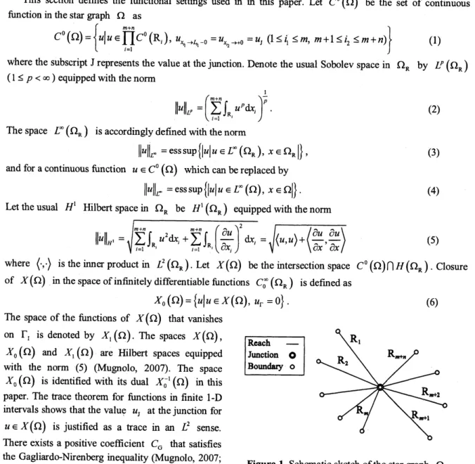
aboundary. Thispaperfocuses

on

aconnected graphthat consistsof

a

finite numberofstraight reaches meetingatajunction$J$(Figure 1), whichis hereafter referred to

as

astar

graph

$\Omega$

.

Thejuncti\‘onattaches

$m$ inflowing reaches($R_{1}$ through $R_{m}$)and $n$ outflowing reaches$(R_{m+1}$ through

$R_{m+n})$

.

The $i$th reach of $\Omega$ is denotedby

$R_{i}$

.

Thelength of $R_{i}$ is $L_{i}<\infty.$ $A$ 1-$D$abscissa isdefinedin

a

reach and that in $R_{j}$ is denotedby

$x_{i}$. The reach $R_{i}$ is thus identified with the 1-$D$ interval $(0,L_{i})$

.

The

junction$J$

can

beregarded

as

thedownstream-ends

of the inflowing reaches$(x_{i}arrow L_{l}-0$ for $1\leq i\leq m)$

as

well

astheupstream-ends (origins)_{of the outflowing reaches}$(x_{i}arrow+0$ for $m+1\leq i\leq m+n)$

.

Theunion_setofthe

reachesof $\Omega$ is denotedby $\Omega_{R}=\bigcup_{i\lrcorner-}^{m+n}R_{i}$. Theunion setoftheupstream

boundaries ofthe inflowing reachesof

$\Omega$ isdenoted by

$\Gamma_{I}$ and that of thedownstreamboundaries of the outflowing reaches by

$\Gamma_{o}$. The boundary

$\Gamma$ of $\Omega$ is thereforedecomposed

as

$\Gamma=\Gamma_{I}\cup\Gamma_{o}.$

2.2 Functional settings

This section defines the functional settings used in in this paper. Let $C^{0}(\Omega)$ be the set ofcontinuous

functionin thestar graph $\Omega$ as

$C^{0}(\Omega)=\{$$u|_{i=1}^{m+n}u\in\Gamma I^{c^{0}}(R_{i}),$ $u_{x_{1}arrow l_{t_{1}}-0}=u_{x_{1}arrow+0}=u_{J}(1\leq i\leq m, m+1\leq i_{2}\leq m+n)\}$ (1)

where the subscript$J$representsthe valueatthe junction. Denote the usual Sobolevspace

in $\Omega_{R}$ by $L^{p}(\Omega_{R})$ $(1\leq p<\infty)$equipped with the

nonn

$\Vert u\Vert_{L^{p}}=(\sum_{i=1}^{m+n}\int_{R_{}}u^{p}dx_{i})^{\frac{1}{p}}$

(2)

The space $L^{\infty}(\Omega_{R})$ isaccordingly

defined

withthenorm

$\Vert u\Vert_{L^{\infty}}=$ess$sup\{|u|u\in L^{\infty}(\Omega_{R}),$ $x\in\Omega_{R}|\}$, (3)

and fora continuous function $u\in C^{0}(\Omega)$ whichcanbe replaced by

$\Vert u\Vert_{L^{\infty}}=$esssup$\{|u|u\in L^{\infty}(\Omega),$ $x\in\Omega|\}$. (4)

Let the usual $H^{1}$ Hilbertspace in

$\Omega_{R}$ be $H^{1}(\Omega_{R})$ equipped with the

norm

$\Vert u\Vert_{H^{1}}=\sqrt{\sum_{t\overline{-}1}^{m+n}\int_{R}u^{2}dx_{l}+\sum_{i--1}^{m+n}\int_{R}(\frac{\partial u}{\partial x_{j}})^{2}dx_{i}}=\sqrt{\langleu,u\rangle+\langle\frac{\partial u}{\partial x},\frac{\partial u}{\partial x}\}}$

(5)

where $\langle\cdot,\cdot\rangle$ is theinnerproduct in

$L^{2}(\Omega_{R})$. Let $X(\Omega)$ be theintersection space $C^{0}(\Omega)\cap H(\Omega_{R})$.Closure

of $X(\Omega)$ in thespaceofinfinitely differentiable functions $C_{0}^{\infty}(\Omega_{R})$ is defmedas

$X_{0}(\Omega)=\{u|u\in X(\Omega),$ $u_{\Gamma}=0\}$ . (6)

The space of the functions of $X(\Omega)$ thatvanishes

on $\Gamma_{I}$ is denoted by $X_{1}(\Omega)$

.

The spaces $X(\Omega)$,

Reach –

$X_{0}(\Omega)$ and $X_{1}(\Omega)$ are Hlbert spaces equipped Junction _$0$

with the

norm

(5) (Mugnolo, 2007). The space Boundary $0$

$X_{0}(\Omega)$ is identifiedwith its dual $X_{0}^{-1}(\Omega)$ inthis

paper. The trace theorem for functions infinite 1-$D$

intervals

shows that the value $u_{J}$ atthe junction for

$u\in X(\Omega)$ is justified

as

a trace in

an

$L^{2}$

sense.

Thereexists apositive coefficient $C_{G}$ that satisfies

theGagliardo-Nirenberg inequality(Mugnolo,2007;

(3)

Berkolaiko

andKuchment,2012)

$\Vert u\Vert_{L^{\Phi}}\leq\sqrt{C_{o}}\Vert u\Vert_{H^{1}}$ (7)

with $C_{G}>0$

.

Let $L^{p}(0,T;H)$ witha finite $T>0$ _{denote the} spaceof temporally $L^{p}$ class functions from

$(0,T)$ intoaHilbertspace $H$

.

Thespace $L^{p}(0,T;H)$ $(1\leq p<\infty)$ is equipped with the

norm

$\Vert u\Vert_{L^{p}(0,T.H)}=(\int_{0}^{T}\Vert u\Vert_{H}^{p}dt)^{\frac{1}{p}}$

(8)

Similarly, thespace $L^{\infty}(0,T;H)$ isequippedwith the

norm

$\Vert u\Vert_{L^{\infty}(0,T.H)}=$

ess

$sup\{\Vert u\Vert_{H}|t\in(0,t)\}$. (9)

3

Burgerstype equation(BTE)model

3.1

Model description

Water

wave

propagationsin

open

channels

are

reasonablycharacterized with

a

BTEmodel,

a

parabolic PDE

having

a

nonlinear advectionterm.Typical form of the model is

$\frac{\partial h}{\partial t}+\frac{\partial}{\partial x}(\frac{1}{M+1}m^{M+1}-D\frac{\partial h}{\partial x})=\frac{\partial h}{\partial t}+\frac{\partial q}{\partial\kappa}=0$ (10)

with theunitwidth discharge ofwater $q$ defined

as

$q=q(h)= \frac{1}{M+1}m^{M+1}-D\frac{\partial h}{\partial x}$ (11)

where thedependentvariable $h=h(t,x)$ represents thewaterdepthitsfluctuation, $V>0$

and

$D>0$

are

_the

model parameters assumed

as

reach-distributed constant and $M\geq 0$ is another model parameter relatedwith

friction laws (Sing, 1996). For example, $M=1$ in Onizukaand Odai (1998), and $M=0.666$ inMizumura

(2010).Inthispaper,theseparameters

are

assumedtobeboundedasin the literatures. The BTE model (10) with

the particular choice of $M=0$ loses the nonlinearity and is regarded

as

a solute transport equation of a

contaminantinwhich $h,$ $V$ and $D$

are

understood

as

theconcentrationofthe contaminant,thefluid velocity

and thedispersioncoefficient,respectively(Yoshioka et al.,inpress).

3.2

Internal boundarycondition (IBC)

Amajor mathematical and numerical difficultyinsolvingthe BTE model (10) on aconnected graphisthe

existenceofjunctions, whichrequire the

use

of appropriate BCs

so

thattheproblemiswell-posed. The IBCs

are

also referred to

as

the Kirchhoffs conditions

or

the transmissive conditions in the literatures (Lumer, 1980;

Pokomyi andBorovskikh,2004).Influencesofthe IBCs

on

propertiesof solutions toPDEs

on

connectedgraphs

have extensivelybeen studied, inparticular for the spectral theory(Carlson, 2009),solvabilityandmultiplicity

theory (Von Below, 1986; Lubary, 1998), semi-group theory (Mugnolo, 2007) and relations with stochastic

processes (FriedlinandSheu, 2000). The authors used

an

analytical approach for parabolicPDEs

on

connected

graphs based

on

the weak forms that implicitly incorporatethe IBCsto investigate mathematical properties of

the PDEs andtodevelopefficient numericalmethodsfor solvingthem(Yoshiokaet al.,2012).

In thispaper, a similaranalyticalmethodis presentedto dealwith the BTE model (10) consistently

on

the

star graph $\Omega$. The model (10)

on

$\Omega$ shall be understood

as

a weak form

so

that thejunction $J$ in $\Omega$ is

consistently dealtwith. The weak form of(10) is givenby

$\sum_{i=1}^{m+n}\int_{R_{J}}[w\frac{\partial h}{\partial t}-\frac{\partial\eta\nu}{a_{i}}(\frac{1}{M+1}V_{f}h^{M+1}-D_{i}\frac{\partial h}{\partial x_{l}})]dr_{i}=t\int_{R_{l}}i=1(w\frac{\partial h}{\partial t}-\frac{\partial w}{\partial x_{i}}q_{t}(h))$ dr,$=0$ (12)

wherethe value of $h$ isdirectlyspecifiedon $\Gamma_{I}$ ($D$chlet boundarycondition)and the free outflow condition

$D=0\underline{\partial h}$

(13)

$/\partial x_{t}$

is assumed

on

$\Gamma_{o}$ (Neumannboundarycondition).No boundary termis embodied in (12).Hereafter,the weak

form (12) is regarded

as

the BTE model. Accordingto Cecchi etal. (1996) and Clark etal. (2011), the 1-$D$

counterpart of(12) is well-posed and hasaunique weak solution with $H^{1}$ regularity. Theparameters

$V_{t}>0$

(4)

theconstraint

$\Delta V=\sum_{j=m+1}^{m+n}V_{;}-\sum_{j=1}^{m}V_{i}=0$, (14)

which is understood

as a

balancelaw of $V_{i}$ around the junction J. The constraint

(14) for the linear

case

of

contaminanttransport$(M=0)$

means

_{physically that}

_mass

_conservation _of_water_{in terms of the discharges is}

satisfiedat$J$(Oppenheimer,2000;Yoshioka

et al.,inpress).Theconstraint (14) isessentialin ordertoguarantee

the

energy estimate

andthe

maximum

principleof the BTEmodel

as

shown inthelater sections.

The BTE model (12) implicitly

assumes an

IBCatthejunction J. The IBCisnotembodied in (12) andis referred to

as

the implicit IBC (Yoshiokaet al., 2013), which is equivalent to the conventional ones for the

solution $h$ ifitssufficientregularityis_guaranteed.

By (14),arepresentationformulafor the IBCis obtained

as

$\sum_{i=1}^{m}q_{i}(h)|_{\chi_{}arrow L_{l}-0}-\sum_{i=m+1}^{m+n}q_{i}(h)|_{\chi,arrow+0}=\sum_{;=1}^{m}D_{i}\frac{\partial h}{\ _{i}}|_{x,arrow L_{l}-0}- \sum_{i=m+1}^{m+n}D_{i}\frac{\partial h}{\ _{\dot{z}}}|_{x_{t}arrow*\mathfrak{v}}=0$ . (15)

The IBC (15) describesa

mass

conservationlaw of wateratthe junction$J$for

a

nonlinear

case

_{$(M\geq 1)$}and that

ofacontaminantfor the linear

case

$(M=0)$

.

_{Each partial}_derivatives_in₍₁₅₎_is_{understood in the}

_sense

_of

_a

_trace

because the space ofdifferentiable functions $C^{1}(\overline{R_{i}})$ is dense in _{$H^{1}(R_{i})$} (Salsa, 2009).

The IBC (15) is

satisfiedin astrong

sense

for the solution $h$ in $H^{2}(\Omega_{R})$

.

4 SolvabilityofBTE $m$odel

on

connected graph

The objective ofthis section is toprove unique

existence

ofthe weak solution $h$ under the homogenous

$D$ chlet boundary conditions. The

parameter $M$ is assumedto equal to

or

larger_than

1.

_{The proofs}_presented

in this section

can

also be applied to the problems with other boundary conditions, such

as

the homogenous

Neumannboundarycondition (13).Here, (12) _{is rewritten in}_{the abstract fom}

$\langle w,\frac{\partial}{\partial t}h\}+a(w,h)+b(w,h,h)=0$ ₍₁₆₎

withthebi-linearform

$a(w,h)= \sum_{\}=1}^{m+n}\int_{R_{1}}D_{i}\frac{\partial w\partial h}{\partial x_{l}\partial\kappa_{l}}dx_{i}$ (17)

andthe(non-linear)operatorform

$b(w,u,v)=- \sum_{i=1}^{m+n}\int_{R_{1}}\frac{1}{M+1}V_{i}\frac{\partial w}{\partial x_{i}}u^{M}vdx_{i}$ . (18)

Here also considers thesteadycounterpart

$a(w,h)+b(w,h,h)= \int_{\Omega}$$wfdx=\langle w,f\rangle$ ₍₁₉₎

with

a

source

$f$,whichisindependentofthe solution $h.$

4.1

Steady problem

This sectionproves unique solvabilityofthe steady problem (19) for $h\in X_{0}(\Omega)$ with $w\in X_{0}(\Omega)$

.

The

proofs presentedin this sectionareinspired by Boules (1990)whopresentedunique solvability ofaBTE model

$(M=1)$in a 1-$D$interval.Define theupper_and_{lower bounds of}

$V_{i}$

as

$\overline{V}=\max_{1\leq i\leq m+n}V_{i}$ and

$\underline{V}=\min_{1\leq i\leq m+n}V_{i}$, (20)

respectively Similarly,definetheupperand lower boundsof $D_{j}$ as

$\overline{D}=\max_{1\leq i\leq m+n}D_{i}$ and

$\underline{D}=\min_{\lrcorner 1<\leq m+n}D_{i}$, (21)

respectively Several important properties ofthebi-linearform $a$ andtheoperatorform $b$

are

presented.The

bi-linearform $a$ satisfies

$|a(w,h)|=| \sum_{i=1}^{m+n}\int_{R},$$D_{i} \frac{\partial w\partial h}{\partial x_{i}\partial_{X_{;}}}dx_{i}|\leq\overline{D}\Vert\frac{\partial w}{\partial x}\Vert_{L^{2}}\Vert\frac{\partial h}{\partial x}\Vert_{L^{2}}\leq\overline{D}\Vert w\Vert_{H^{1}}\Vert h\Vert_{H^{1}}$

(22) and

(5)

$a(u,u)= \sum_{i=1}^{m+n}\int_{R_{J}}D_{i}(\frac{\partial u}{\ })^{2} dx_{l}\geq\underline{D}\Vert\frac{\partial u}{\ } \Vert_{L^{2}}^{2}\geq a\Vert u\Vert_{H^{1}}^{2}$ (23)

for $u\in X(\Omega)$ with a somepositive constant $a$, showing that it is bounded and coercive (Mugnoro, 2007).

The operator form $b$ isalso bounded for $u\in X_{0}(\Omega)$

.

In

fact

according tothe Sobolev embedding theorem

(Tartar, 2000),the inequality

$|b(w,u,v)|=| \sum_{i=1}^{m+n}\int_{R_{1}}V_{i}\frac{\partial w}{\partial x}u^{M}vdx_{l}|\leq\beta\Vert w\Vert_{H^{1}}\Vert u\Vert_{H^{1}}^{M}\Vert v\Vert_{H^{1}}$ (24)

with $\beta=\overline{V}(C_{G})^{\frac{M}{2}}>0$ holds. Definethe operator $\lambda(u,v)\in X_{0}(\Omega)$ via theinnerproduct

$b(w,u,\nu)=\langle\lambda(u,v),w\rangle$, (25)

and denote $\lambda(u,u)$ by $\lambda(u)$

.

The

norm

of $\lambda(u)$ is givenby

$\Vert\lambda(u)\Vert=\sup\{\frac{\langle\lambda(u),w\rangle}{\Vert w\Vert_{H^{1}}}w\in X_{0}(\Omega),$$w\neq 0\}\leq\overline{V}(C_{G})^{\frac{M}{2}}\Vert u|\ovalbox{\tt\small REJECT}_{l}=\beta\Vert u|\kappa_{1}$ , (26)

showing that $\lambda(u)$ is bounded for $u\in X_{0}(\Omega)$ Furthemore, $\lambda(u)$ is continuous. In fact, for

$u_{1},u_{2}\in X_{0}(\Omega)$ the inequality

$\Vert\lambda(u_{1})-\lambda(u_{2})\Vert=\sup\{\frac{\langle\lambda(u_{1})-\lambda(u_{2}),w\rangle}{\Vert w\Vert_{H^{I}}}w\in X_{0}(\Omega),$ $w \neq 0\}\leq\overline{V}\sum_{j=1}^{M-1}\Vert u_{1}\Vert_{\Gamma}^{j}\Vert u_{2}|\beta_{\Phi}^{-1-1}\Vert u_{1}-u_{2}\Vert_{L^{\infty}}$ (27)

issatisfiedbecause $\overline{V}\sum_{j=1}^{M-1}\Vert u_{1}\Vert_{L^{\infty}}^{J}\Vert u_{2}|\psi_{L^{Q}}-j-1$ isbounded.

Before staltingthemainproof,

a

uni-variatefunction $g=g(r)$ with $r\geq 0$ and $M$,defined by

$g(r)=r(a-\beta r^{M})$ (28)

is introduced.The function $g$ satisfies

$g(O)=g(r_{0})=0$ with $r_{0}=( \frac{\alpha}{\beta})^{\frac{1}{M}}$

(29)

$\frac{d}{dr}g(r_{1})=0$ with $r_{1}=( \frac{a}{\beta(M+1)})^{\frac{1}{M}}$ and $g(r_{1})= \frac{M}{\beta^{\frac{1}{M}}}(\frac{\alpha}{M+1})^{\frac{M+1}{M}}$ (30)

The function $g$ is strictly positive in $(0,r_{0})$ and attains its maximal at $r=r_{1}<r_{0}.$ $g$ monotonically

increasesand decreasesin $(0,r_{1})$ andin $(r_{1},r_{0})$,respectively Itfollows that theequation

$r(\alpha-\beta\mu)=\overline{g}$ (31)

withthe constant $g$ satisfying

$0<\overline{g}<g(r_{1})$ . (32)

has twopositivesolutions $r_{m}$ and $r_{M}$ such that

$0<r_{m}<r_{1}<r_{M}<r_{0}$. (33)

Herefirstlyprovesthe followingtheorem.

Theorem 1.There existsauniquesolution $u\in X_{0}(\Omega)$ tothe linearproblem

$a(w,v)+b(w,h,\nu)=(w,f\rangle (34)$

(6)

$\Vert h\Vert_{H^{1}}<r_{m}$ (35)

holds where $w\in X_{0}(\Omega)$ isthe weight, _{$f\in X(\Omega)$} isa sufficiently regular

source

_term

such that

$\Vert f\Vert=\overline{g}=\sup\{\frac{\langle f,w\rangle}{\Vert w\Vert_{L^{2}}}w\in X_{0}(\Omega),$_{$w\neq 0\}\leq g(r_{m})$}

(36) with

$K= \frac{\beta Mr_{m}^{M-1}\Vert f\Vert}{(\alpha-\beta r_{m}^{M})^{2}}<1$

.

(37)

Notethat $r_{m}$ depends onlyon $f,$ $\alpha,$ $\beta$ and $M.$

Proof of

Theorem 1.

Theset

$D(r_{m})=\{h|h\in X_{0}(\Omega),$ $\Vert h\Vert_{H^{1}}<r_{m}\}$ (38)

isacompact,

convex

subset of $X_{0}(\Omega)$.By (23) and (24),the left hand sideof (34) is bounded from

zero

as

$a(v,v)+b(v,h,v)\geq\alpha\Vert v\Vert_{H^{1}}^{2}-\beta\Vert v\Vert_{H^{1}}^{2}|h\Vert_{H^{1}}^{M}=(\alpha-\beta\Vert h\Vert_{H^{1}}^{M})\Vert v\Vert_{H^{1}}^{2}\geq(\alpha-\beta r_{m}^{M})\Vert v\Vert_{H^{1}}^{2}$, (39)

showingthatitis coercive.Application of the Lax-Milgram Theorem(AtkinsonandHan,2009)to (34) leads to

that thesolution $v\in X_{0}(\Omega)$ existsandisuniquelydetermined.

Here secondlyprovesunique solvability of(19) under the stated conditions.

Theorem

2.

(19) hasauniquesolution $h\in X_{0}(\Omega)$ under the stated conditions.

Proof of

Theorem

2.

Denote $\Phi(h)$ by the map identified with the inverse of

the

_operator $A_{h}$, which is

definedvia the innerproductas

$\langle A_{h}v,w\rangle=a(w,v)+b(w,h,v)$ , ₍₄₀₎

namely,

$\Phi(h)=(A_{h})^{-1}f$ . ₍₄₁₎

Theoperator

norm

of $A_{h}$ satisfies

$\Vert A_{h}v\Vert=\sup\{\frac{|a(w,v)+b(w,h,v)|}{\Vert w||_{H^{1}}}w\in X(\Omega),$$w \neq 0\}\geq\frac{a(v,v)-|b(v,h,v)|}{\Vert v||_{H^{1}}}\geq(\alpha-\beta r_{m}^{M})\Vert v\Vert_{H^{1}}$

.

(42)

Since $A_{h}$ is bijectivebythe defmition, it isanopenmap.Applicationof

the open-mapping theorem(Okamoto

andNakamura, $1997a$₎_to $A_{h}$ yields theestimate

$\Vert(A_{h})^{-1}\Vert\leq\frac{1}{\alpha-\beta r_{m}^{M}}$, (43)

which further leadsto

$\Vert(A_{h_{1}})^{-1}-(A_{h_{2}})^{-1}\Vert\leq\frac{1}{(\alpha-\beta r_{m}^{M})^{2}}\Vert A_{h_{1}}-A_{h_{2}}\Vert$

.

(44)

Application ofadifferentialformulato $A_{h}$ yields

$\Vert A_{I}-A_{h_{2}}\Vert=\sup\{$

$\leq\overline{V}C_{G}$

$\frac{|a(w,v)+b(w,h_{7},v)-a(w,v)-b(w,h_{\eta},v)|}{||v||_{H^{1}}\Vert w||_{H^{1}}}v,w\in X(\Omega),$_{$v,w\neq 0\}$}

.

(45)

$\frac{1}{2}\sum_{j=0}^{M-1}\Vert h^{j}\Psi^{-j-1}\Vert_{L^{\infty}}\Vert h-h_{2}\Vert_{H^{1}}$

By (35), (45) resultsin

(7)

showingthat $A_{h}$ is continuous. Consequently, $\Phi$ is

a

contraction

map

that

maps

_$X(\Omega)$ onto _$X(\Omega)$

.

This

isbecause,by (36) and (39), $\Vert\nu\Vert_{H^{1}}$ is bounded from awayas

$\Vert v\Vert_{H^{1}}\leq\frac{\Vert f\Vert}{\alpha-\beta r_{m}^{M}}\leq\frac{g(r_{m})}{\alpha-\beta r_{m}^{M}}=r_{m}$ (47)

andby (37), (44) and (45), $\Phi$ satisfies theinequality

$\Vert\Phi(h_{r})-\Phi(h_{\eta})\Vert<\Vert h-h_{2}\Vert_{H^{1}}$

.

(48)

According to the Leray-Schauder fixed point theorem $($Okamoto $and$ Nakamura, $1997b)$, the solution

$h\in X_{0}(\Omega)$ to (19) existsandisuniquely determined under the stated conditions.

Here finallyprovesthefollowingtheorem.

Theorem

3.

(19) doesnothaveanysolutions such that

$r_{m}<\Vert h\Vert_{H^{1}}<r_{M}$. (49)

Proof of Theorem

3.

Substituting $w=h$ into (19) yields

$a(h,h)+b(h,h,h)=\langle w,f\rangle$, ₍₅₀₎

leadingtothe inequality

$(\alpha-\beta\Vert h|\beta_{1})\Vert h\Vert_{H^{1}}\leq\Vert f\Vert$

.

(51)

Substituting (36) into (51) yields

$(\alpha-\beta\Vert h\Vert_{H^{1}}^{M})\Vert h\Vert_{H^{1}}\leq g(r_{m})$ . (52)

Since $r_{m}$ and $r_{M}$

are

thesolutionsto (31),theassumption (49) contradicts withthe inequality (52) showing

that thestatementistrue.

It

can

beshown

in

an

essentiallysimilarwaythatthe solution $h\in X_{0}(\Omega)$ totheweak form

$a(w,h)+b’(w,h,h)+c(w,h)+d\langle w,h\rangle=\langle w,f\rangle$ ₍₅₃₎

withapositiveconstant $d$ and theoperatorform

$b’(w,u,v)=- \sum_{t=1}^{m+n}\int_{R_{J}}\frac{\partial w}{\partial\kappa_{t}}(\frac{1}{j+1}\sum_{/\overline{-}1}^{M}V_{l.j}u^{j})vdx_{l}$ (54)

with

a

positive and bounded

sequence

$V_{i.j}$,has

a

unique solution $h\in X_{0}(\Omega)$ suchthat $\Vert h\Vert_{H^{1}}^{2}<M^{-1}r_{m}^{M}$

.

Note

that the analysis camiedoutinthissectiondoes not

assume

theconstraint (14),which

on

the other hand

serves as

a

crucial condition that determinespropertiesof solutionstothe unsteady BTE model.

4.2

Unsteadyproblem

4.2.1

Energy

estimate

Energyestimateof the problem (16) is obtainedusing theFaedo-Galerkinmethod,which

ensures

theglobal

uniqueexistence ofthesolution $h.$

Theorem 4. Theenergyestimate

_of

(16) isderivedas

$\frac{1d}{2dt}\Vert h\Vert_{L^{2}}^{2}+\alpha\Vert h\Vert_{H^{1}}^{2}\leq 0$

.

(55)

Proof of Theorem

4.

Denote $W$ by

a

separable base of linearlyindependent elementsof $X_{0}(\Omega)$

.

Consider

linearly independentelements $h_{k}$ $(k=1,2,3\ldots)$ in $L^{2}(0,T;X_{0}(\Omega))$ defined

as

$h_{k}= \sum_{j=1}^{k}p_{/}w_{jk}(t)$ (56)

(8)

fromthe ordinary differential equations(ODEs)

$\{p_{j_{1}},\frac{\partial}{\partial t}h_{k}\}+a(p_{j_{1}},h_{k})+b(p_{j_{1}},h_{k},h_{k})=0,1\leq j_{1}\leq k$ ₍₅₇₎

with the initial condition

$h_{\eta}(t=0)=h_{k,0}$ ₍₅₈₎

where $h_{k,0}$ is

a

orthogonal projection of _{$h\in L^{2}(0,T;X(\Omega))$} to _$W$

.

Thesquare matrix

constructed from the

coefficients ofthe first term ofthe left hand side of (57) is

a

Gram matrix. The Peano’s existence theorem

(Hartman, 2002) _{shows that the approximate solution} $h_{k}$ exists and is uniquely determined atleast locally in

$(0,T)$._Multiplying ₍₅₇₎ _by $\omega_{jk}$ and assembling it for $1\leq j\leq k$ yields

$\langle h_{k},\frac{\partial}{\partial t}h_{k}\rangle+a(h_{k},h_{k})+b(h_{k},h_{k},h_{k})=0$

.

(59)

By (14),_{the third term ofthe left hand side of} (59) vanishes

as

$b(h_{k},h_{k},h_{k})=- \frac{1}{M+1}\sum_{i=1}^{m+n}V_{i}\int_{R_{l}}\frac{\partial h_{k}}{\partial x_{i}}W_{k}^{+1}dx_{i}=-\frac{1}{(M+1)(M+2)}\Delta Vh_{k,J}^{M+2}=0$, (60)

leading to theenergy inequality

$\frac{1}{2}\frac{d}{dt}\Vert h_{k}\Vert_{L^{2}}^{2}\leq-\alpha\Vert h_{k}\Vert_{H^{1}}^{2}$.

(61)

Integrating (61) from $t=0$ _to _$t=T>0$ _{yields the}_{energy estimate}_of $h_{k}$

as

$\frac{1}{2}\Vert h_{k}(T)\Vert_{L^{2}}^{2}+\int_{0}^{T}\alpha\Vert h_{k}\Vert_{H^{1}}^{2}dt\leq\frac{1}{2}\Vert h_{k,0}\Vert_{L^{2}}^{2}$ ,

(62)

showing that $h_{k}$ remains inaboundedsetof _{$L^{\infty}(0,T;L^{2}(\Omega))$}

.

Since

(62) leadsto

$\max_{0\leq t\leq T}\{\Vert h_{k}(T)\Vert_{L^{2}}^{2}+\int_{0}^{t}\alpha\Vert h_{k}\Vert_{H^{1}}^{2}dt\}<\infty$, (63)

$h_{k}$ remains in a bounded set of _{$L^{2}(0,T;X_{0}(\Omega_{R}))$} . Ascoli-Arzela theorem

shows that there exists a

subsequence $h_{k}$, that

converses

to $h$ weakly in _{$X_{0}(\Omega)$} and thus there exists a unique

solution

$h\in L^{2}(0,T;X_{0}(\Omega))\cap L^{\infty}(0,T;L^{2}(\Omega_{R}))$ by(7). The classical_compactnesstheorem_{(Temam, 1997)}

ensures

_that

the convergence of $h_{k}$ to $h$ is also achieved in the space _{$L^{2}(0,T;L^{2}(\Omega_{R}))$} in a _strong

sense because the

operatorform $b$ definesa continuousand bounded fimction

$\lambda(h)$ for $h\in X_{0}(\Omega)$.The resultin$g$solution $h$

to (16) satisfies (55),which finishes theproof Note also that the inequality

$\frac{1d}{2dt}\Vert h\Vert_{L^{2}}^{2}+\alpha\Vert h\Vert_{L^{2}}^{2}\leq 0$

(64)

follows from theenergy estimate (55),showing that $h$ approaches$0$intheentire $\Omega$ in the $L^{2}$

sense.

4.2.2 Maximum

principle

Herea maximumprinciple ofthe BTE model (16) ispresented.

Theorem 5. (16)

_satisfies

_{thefollowing maximum}_principle

_for

_any $T>0,\cdot$

$\Vert h\Vert_{L^{\infty}(\Omega_{R}x(0,T))}<H$ if $\Vert h\Vert_{L^{\infty}(\Omega_{R})}<H<\infty$ (65)

Proof ofTheorem 5.Defineanon-negative functions $f^{+}$ and $f^{-}$ foragenericfunction _$f$ as

$f^{+}= \max\{f,0\}$ and $f^{-}=- \min\{f,0\}$, ₍₆₆₎

respectively Substituting $w=(h-H)^{+}\in X_{0}(\Omega)$ and $u=v=h$ _into $b$ yields

$b((h-H)^{+},h,h)=- \sum_{i=1}^{m+n}\int_{R_{l}}\frac{1}{M+1}V_{i}\frac{\partial(h-H)^{+}}{\partial x_{t}}h^{M+1}dx_{1}$. (67)

Applicationofthe binomial theoremto $h^{M+i}$ yields the polynomial expansionin

(9)

$\Psi^{+1}=(h-H+H)^{M+1}=\sum_{j=0}^{M+1}(\begin{array}{l}M+1j\end{array})(h-H)^{1}H^{M+1-j}$

.

(68)

Substituting (68) into (67) leadsto

$b((h-H)^{+},h,h)=- \frac{1}{M+1}\sum_{\dot{j}=0}^{M+1}H^{M+1-j}(\begin{array}{l}+lMj\end{array})\sum_{t=1}^{m+n}V,\int_{R_{J}}\frac{\partial(h-H)^{+}}{\partial \mathfrak{r}_{i}}(h-H)^{j}dx,$

.

(69)

By (66),the equality

$\int_{R_{J}}\frac{\partial(h-H)^{+}}{\partial x_{i}}(h-H)^{j}dx_{i}=\int_{R_{l}}\frac{1\partial}{j+1a_{i}}[(h-H)^{+}]^{J+1}dx_{1}=[\frac{1}{j+1}[(h-H)^{+}]^{j+1}]_{\eta=0}^{\eta=A}$ (70)

holds. Substituting (70) into (69) resultsin

$b((h-H)^{+},h,h)= \frac{\Delta\nabla}{M+1}\sum_{j=0}^{M+1}H^{M+1-j}(\begin{array}{l}M+1j\end{array})\frac{1}{j+1}[(h_{J}-H)^{+}]^{J+1}=0$. (71)

In addition,

since

$a((h-H)^{+},h)= \sum_{j=1}^{m+n}\int_{R_{l}}D_{l}\frac{\partial}{\partial x_{l}}(h-H)^{+}\frac{\partial h}{\partial x_{1}}$dx, $= \sum_{j=l}^{m+n}\int_{R_{t}}D_{i}[\frac{\partial}{\partial x_{l}}(h-H)^{+}]^{2}dx_{l}\geq 0$ (72)

holds,substituting (71) and $\langle$72) into (16) obtains theestimate

$\langle(h-H)^{+},\frac{\partial}{\partial t}h\}=\frac{1}{2}\frac{d}{dt}\Vert(h-H)^{+}\Vert_{L^{2}}^{2}=-a((h-H)^{+},h)\leq 0$ , (73)

which leadsto

$\Vert(h-H)^{+}\Vert_{L^{2}}^{2}\leq\Vert(h_{0}-H)^{+}\Vert_{L^{2}}^{2}=0$, (74)

showing that $h<H$ in $\Omega x(0,T)$

.

Similarly, taking $w=-(h-H)^{-}$ in (16) yields $h>-H$ in $\Omega x(0,T)$

and thus the statement isproven.An importantconsequenceofthemaximumprincipleisthat the solution witha

non-negative initial condition $h_{\tau}\in X_{0}(\Omega)$ remains non-negativefor arbitrary $t>0.$

5.

Numerical analysis

on

the BTE model

5.1

ConformingPetrov-Galerkin

finite

element method

Numerical analysis

on

theBTE model iscarniedout tofurtherinvestigatebehaviourofits solutions. Dhawan

etal. (2012)reviewed numericalmethods for BTE models. Although theyextensively surveyed the numerical

methods, the models

on

connected graphs

were

not focused

on.

Some authors developed practical numerical

methodstosolve PDEs on connectedgraphs; however,their methods do necessarilynotguarantee regularity of

the solutions at junctions (Islam and Chaudhry, 1998; Basha and Malaeb, 2007; Tumanova, N., and

\v{C}iegis,

2012). The authors developed

a

conformingPetrov-Galerkm finite elementmethod(CPGFEM)that solves the

BTEmodel (12) using weight and interpolationfunctions in $X(\Omega)$ and $X_{0}(\Omega)$ (Yoshiokaet al.,2013).

5.2

Test problems

Testproblems

are

firstlyconsideredto showthatthe condition (14) isessential for themaximumprinciple.

Herethe parameter $M$ isset

as

2.Alocally 1-$D$ open channelnetwork $\Omega$

as

showninFigure2isset

as

the

computational domain. The key nodes defining the boundaries of the reaches are labeled from A through $E,$

whicharethe upstream-end(A),

downstream-ends

($C$andD)and ajunction(B).Length of each reach equals to

1.The reachesA-B,B-$C$andB-$D$

are

labeled

as

$R_{i},$ $R_{2}$ and $R_{3}$,respectively. $D$ isset

as

0.001 intheentire

$\Omega$

.

Here the following two

cases

of $V_{i}$

are

considered.

(a) $V_{1}=3.0,$ $V_{2}=2.0$ and $V_{3}=1.0$ (Thecondition (14) issatisfied)

(b) $V_{1}=3.0,$ $V_{2}=1.0$ and $V_{3}=0.5$ (Thecondition (14) isnotsatisfied:$\Delta V<0$)

(c) $V_{1}=3.0,$ $V_{2}=4.0$ and $V_{3}=2.0$ (Thecondition (14) isnotsatisfied:$\Delta V>0$)

The initial condition is $h=1$ in the entire $\Omega$ . The homogenous Dirichlet boundary condition $h=0$ is

(10)

temporalintegrationprocedurearenegligible small.

Figures $2(a)-(c)$ plot the computational results of $h$ for each

case

at _{$t=500i\Delta t$} with $i$ the integer,

clearly showing that themaximumprincipleisviolatedinthe

case

(b) ($h$ exceeds 1 in $\Omega$).Inthe

case

(c),the

maximumpninciple isnotviolated but the solution has

an

abrupt changeat$B$, whichis not observed in the

case

(a). Inall the

cases

ararefaction

wave

propagatesfrom $\eta$ to $R_{2}$ andto $R_{3}$, andshocks resulting from the

homogenous$D$chletboundary condition

are

created

near

$C$and D.

5.2

Real problem

The BTEmodel

as

a

goveming equation ofthe waterdepth fluctuation is applied tosimulate water

wave

propagations in

an

agricultural drainage system in Japan. The computational domain is

same

with that ofin

Yoshiokaetal. (2014). Figures3shows

a

sketch of thedomain $\Omega$, whichisidentified with aconnected graph

having five reaches andtwojunctions. An underlying water flowtodetermine the coefficients of the BTEmodel

is computedonthe basis ofauniform depth formulaatthe boundaries$AB$and$C$,respectively The boundary

conditions

are

the Dirichletone $h=0.1$ (m)at$AB$and$C$and

a

Ree-outflowoneatD.Here, $V$ issetas

$V= \frac{2}{3}\sqrt{g}[(h+h)^{\frac{3}{2}}-h^{\frac{3}{2}}]$ (75)

where $g$ is thegravitational acceleration and

ig

is thewaterdepth of the underlying equilibrium flow field.

The coefficient $V$ in (75) is determined so that the celerity ofthe inviscid counterpart ofthe BTE

model

reducestothat of the non-dispersivegravitational wave $\sqrt{g(h+h_{0})}$. The coefficient $D$ issetas 0.1 $(m^{2}/s)$in

theentire $\Omega.$ $\Delta t$ is0.004(s). Figure4plots waterwavepropagationsin

thedomainat $t=500i\Delta t.$

6 Conclusions

This

paper

_{analytically and numerically studied the BTE model. The homogenous} $D$chlet boundary

condition

was

assumed in this paper _{for the simplicity, but linear non-homogenous conditions}

_can

_{also be}

implemented without any technical difficulties. The mathematical analysis revealed that the BTE model is

well-posed ifthecoefficient $V$ satisfies the balance law (14).Theconstraintwasessentialin order_toobtain the

energy estimate and the maximumpninciple for the model. Another theoretical analysis focusing on a steady

BTE model with a

source

terms revealed that its solution is uniquely determined if the

source

is sufficiently

regular. Numerical simulation camied out with the CPGFEM showed that the solutions totheBTE model have

singularbehaviouraroundthe unction$J$if (14) isnotsatisfied.

The analyses carriedoutinthispaperrevealeda$paIt$ ofthe basic properties ofthe BTE model. Thispaper

a

priori assumed the constraint (14) as a sufficient condition in order to obtain the

energy

estimate and the

Maximum principle.However,itisnot

sure

atthepresentwhether it also

serves as a

necessarycondition

or

not.

In addition, thispaper does not

cover

the models withnonlinear source terms as discussed in the researches

(Tersenov, 2010;2012).Furthermore,thereexistsaBTEmodelhavinga degenerate diffusion term(Mizumura,

2010)whosesolutionsareexpectedtobehave

more

irregularly than the non-degenerate counterparts, which also

serves as an

effective _{reduced mathematical model of the 1-D SWEs. Future research will focus}

_on

investigations of the well-posedness andmathematical properties of the extended BTE models on connected

graphs, suchasthe

ones

withadegenerate diffusionterm$and/or$a_non-linear

source

_term.

Acknowledgements

Thisresearchissupported by the JapanSociety forthePromotionofScienceundergrant No.$25\cdot 2731$

.

The

authors thankto _{participants of the RIMS Conference: Mathematical Aspects and Applications} _of_Nonlinear

Wave Phenomena for their helpful suggestions and comments. References

[1] _{Atkinson, K., and}Han,W.(2009):TheoreticalNumerical Analysis,Springer, pp.277-365.

[2] _{Barker, B., Johnson, M.A., Noble,}P., Rodrigues, L.M., andZumbrun, K. (2010): Whithamaveragedequations and

modulational stability ofperiodic travelingwaves ofa hyperbolic-parabolic balance law, Journ\’ees\’Equations aur

d\’eriv\’ees partielles,pp. 1-24.

[3] Bapat, R.B.(2010):GraphsandMatrices,Springer, pp.11-39.

[4] Basha, H.A, and Malaeb, L.N. (2007): _{Eulerian-Lagrangian method for constituent}_transport _in _water_distribution

(11)

(a) (b) (c)

Figure2.Computational results of the testproblems.

Figure 4.$A$sketch of $\Omega$ forthe real problem. Figure5.Computational results ofthe real problem.

[5] Berkolaiko, G.,andKuchment,P.$(2012)$;_lntroductiontoQuantum Graphs, Applied Mathematical Society, pp.2-35.

[6] Boules, A.N. (1990): On the existence of the solution ofBurgers’ equation for $n\leq 4$, International Journal

of

Mathematics&MathematicalScience, 13(4),pp.645-650.

[7] Bressan, N., and Quarteroni, (1987): Animplicit/explicitspectralmethod for Burgers’ equation,Calcolo,23(3),

pp.265-284.

[8] Bressloff, P.C.,Dwyer,V.M.,andKearmey, M.J.(1997):Burgers’ equationon abranchingstructure,Physics Letters

$A$,229(1),_$pp.37A3.$

[9] Carlson, R. (2009): Spectral theory fornonconservative transmission linenetworks, Networks andHeterogeneous

Media,6(2),pp.257-277.

[10] Cecchi, M.M., Nociforo, R., and Grego, P.P. (1996): Space-time finite elements numerical solution ofBurgers

problems, LeMatematiche,51(1),pp.43-57.

[11] Clark, H.R., Rincon, M.A, and Silva, A. (2011): Analysis and numerical simulation of viscous Burgers equation,

Numerical Functional analysis and optimization,32(7),pp.695-716.

[12] Coclite, G.M.,and Garvello,M. (2010):Vanishingviscosity for trafficonnetworks,SIAMJournal

_{ofMathematical}

Analysis,42(4),pp. 1761-1783.

[13] Cole, J.D.(1951):Onaquasi-linear parabolic equation occurring in aerodynamics,Q.Appl.Math.,9,pp.225-236.

[14] Dhawan, S., Kapoor, S., Kumar, S., and Eawat,S. (2012): Contemporaryreview oftechniquesfor thesolution of

nonlinearBurgersequation, Journal

_of

ComputationalScience,3(5),405-419.

[15] Evans,L.C.(1998):Partial

_Differential

$\Phi$uations,American Mathematical Society, pp.239-428.

[16] Friedlin, M., and Sheu, S. (2000): Di$\Re sion$processes on graphs: Stochastic differential equations,large deviation

principle, Probability Theory and RelatedFields, 116,pp.181-220.

[17] Hartman,P.(2002):Ordinary

_Differential

Equations, SLAM,Philadelphia.

[18] Hopf, E. (1950): The partial differential equation $u,$$+uu_{\chi}-vu_{n}=0$, Communications on Pure and Applied

(12)

[19] Islam, M.R,_{and Chaudhry,} _M.H.(1998): Modelingofconstituenttransportin unsteady flows in pipe networks,$J$

Hydraul.Eng., 124(11),pp. 1115-1124.

[20] Lubary, J.$A$ _(1998): Multiplicity of solutions of second-order linear differential equations

on networks. Linear

Algebra anditsApplications,274,pp.301-315.

[21] Lumer, G., (1980):Conectingoflocaloperatorsand evolution equationsonnetworks,Lecture Notesin Mathematics,

787, pp.219-234.

[22] Mizumura, $K$ (2010): Analytical solution _of_{nonlinear diffusion}_wave _model, _Journal

of

Hydraulic Engineering,

17(7),pp.782-789.

[23] Morikawa, G.K. (1957): _{Non-linear diffusion of flood} _waves _in rivers, _{Communications} on Pure andApplied

Mathematics,10(2),pp291-303.

[24] Mugnoro, D. (2007): Gaussian estimatesforaheat equationona network,NetworksandHeterogeneousMedia, 2,

pp.55-79.

[25] Nasseri, M., and Attarnejad, $K$(2010):Applications of variationaliteration_methodin_{applied hydrology, Journal}

of

Hydrologic Engineering, 14(9),pp.984-991.

[26] Noble,P. (2007): Linearstability of viscous rollwaves, Communications inPartial

_Differential

Equations, 32(11),

pp.1681-1713.

[27] Odai, S.N., Kubo, N., and Osato, K. (2006): Analytical solutionof the Burgers equation forsimulating translator

wavesinconveyancechannels,JournalofHydraulicEngineering,132(2),pp.194-199.

[28] OdaiS. N.,andKubo, N.(2007):TheBurgersequation model and the monoclonalwavephenomenoninconveyance

channels,JournalofHydraulic Research,45(1),pp.62-66.

[29] Oey, L.Y.(2005):$A$wetting and drying scheme for_POM,_{Ocean Modelling,}_9(2),_pp.

133-150.

[30] Onizuka, K.,andOdai,$SN$.(1998): Burgers’equation model for_unsteady_flow_in_open_channels,_{Journal ofHydraulic}

Engineering,124(5),pp.509-512.

[31] Okamoto,H.,and Nakamura, S.$(1997a)$: Functional_{Analysis 1, Iwanami Bookstore, pp.97-119.}

[32] Okamoto,H.,and Nakamura, S.$(1997b)$: FunctionalAnalysis_{2, Iwanami Bookstore,}_{pp. 181-198.}

[33] Oppenheimer, S.F. $(2(K)0)$:$A$ convection-diffusion problemin a _{network, Applied}_{Mathematics and Computation,}

$112(2-3)$,pp.223-240.

[34] Pokomyi, $Y,V$_,, _and _Borovskikh, _$AV$. _(2004): _Differential_equations _on _networks

(Geometric graphs), Journal

_of

MathematicalScience, 119(6),pp.691-718.

[35] Salsa, S.(2009):_Partial

_Differential

_Equations_{in Action,}_Springer,_{pp. 13-101.}

[36] Santillana, M.,andDawson, C. (2010): $A$ numerical approach tostudytheproperties _{of solutions of the diffusive}

waveapproximation ofthe shallowwaterequations, ComputationalGeoscience,14(1),pp.31-53.

[37] Singh, V.P.(1996):KinematicWaveModellinginWater Resources, John Wiley&Sons, Inc.,pp.541-570.

[38] Szymkiewicz, R.(2010):_{Numerical Modeling}inOpen ChannelHydraulics, Springerpublishing.

[39] Tartar,L.(2000):AnIntroductiontoSobolevSpaces$andInterpolation^{}$Spaces, Springer, pp.81-84. [40] Temam,R.(1997):

_{Infmite-dimensional}

DynamicalsystemsinMechanicsand Physics, Springer,pp.82-140.

[41] Tersenov, $AS$. (2010): Onthe generalized Burgers equation, Nonlinear

_Differential

Equations andApplications,

17(4),pp.437-452.

[42] _{Tersenov, A.S.}(2012):$A$condition guaranteeing the absence of the blow-up_phenomenon_for_{the generalized Burgers}

equation,NonlinearAnalysis:Theory,Methods, &Applications,75(13),pp.5119-5122.

[43] Tsai, C.W.S. (2002):Applicabilityof kinematic, noninertia, andquasi-steadydynamicwavemodelsto unsteadyflow

routing, Journal ofHydraulic Engineering, 129(8),pp.613-627.

[44] Tumanova,N.,and

Ciegis,

$R(2012)$_{: Predictor-corrector domain}decompositionalgorithmfor parabolic problemson

graphs, Math.Model. Anal.17(1),pp. 113-127.

[45] Von $B$elow, J. (1986): Classical solvability of _linear _{parabolic equations} on _networks,

Journal

_{of Differential}

Equations,72(2),pp.316-337.

[46] Yen, B.C,, andTsai, C.W.S. (2001): Onnoninertiaversus diffusionwave infloodrouting, Journal

_of

Hydrology,

$244(1-2)$,pp.97-104.

[47] Yoshioka,H., Unami, K.,andKawachi,T.(2012):Partial_{differential equation model for spatially distributed statistics}

ofcontaminant particles _{in locally one-dimensional open} channel networks, Proceedings

_of

Tenth International

Conference

onHydroscienceandEngineering,$24pp.$

[48] Yoshioka, H., Kinjo, N., Unami, K., and Fujihara, M. (2013): $A$ conforming finite element method for

non-conservative advection-diffusionequations on connected graphs,Journal

_of

JapanSociety

_of

CivilEngineers,

Series$A2$_{(AppliedMechanics),}_69(2),_pp._{$I_{-}59-I_{-}70$}_._{(in Japanese)}

[49] Yoshioka, H., Unami, K., and Fujihara, M. lnternal boundary conditions for solute transport equations in locally

one-dimensional open channelnetworks, Journal

_ofRainwater

CatchmentSystems,$9pp$.(in press)

[50] Yoshioka$H$.,Kinjo,N.,Mabaya,G.,Unami, K.,_and_{Fujihara, M.}_(2014):

$A$hyperbolic longitudinaldispersionmodel

of contaminant in open channel networks, Proceedings

_of

the $7^{h}$

International Symposium on Environmental

Hydraulics,$4pp$.(accepted)

[51] Yu, J., and Kevorkian, J. (1992): Nonlinear evolution of small disturbances into roll waves in an inclined open